
Pumpkin Yield Estimation Using Images from a UAV


UAS Center, The Maersk Mc-Kinney Moller Institute, University of Southern Denmark, Campusvey 55, 5230 Odense, Denmark
*
Author to whom correspondence should be addressed.
Agronomy 2022, 12(4), 964; https://0-doi-org.brum.beds.ac.uk/10.3390/agronomy12040964
Submission received: 8 March 2022
/
Revised: 11 April 2022
/
Accepted: 14 April 2022
/
Published: 16 April 2022
(This article belongs to the Special Issue Crop Yield Prediction in Precision Agriculture)
Abstract
:The paper presents a pumpkin yield estimation method using images acquired by a UAV. The processing pipeline is fully automated. It consists of orthomosaic generation, a color model collection using a random subset of the data, color segmentation, and finally counting of pumpkin blobs together with assessing the number of pumpkins in each blob. The algorithm was validated by a manual check of 5% of each tested dataset. The precision value ranges between 0.959 and 0.996, recall between 0.971 and 0.987, and F1 score falls between 0.971 and 0.988. This proves the very high efficiency of the processing workflow and its potential value to farmers.
1. Introduction
Detailed information about the amount and quality of crop plants can help farmers make better decisions when selling crops. Unmanned Aerial Vehicles (UAVs) can collect large amounts of data from farm fields in form of images [1]. To provide value to the farmer, these images need to be interpreted in a suitable way [2].
The task of estimating crop emergence early in the growing season from UAV-acquired images has been addressed in multiple studies. He et al. [3] reviewed the literature about fruit yield detection and classify the topic of this paper, pumpkin counting, as a direction yield estimation technique. Sankaran et al. [4] estimated potato emergence by segmenting normalized difference vegetation index images and counting the number of segmented objects above a certain size. Chen et al. [5] performed spectral-based segmentation to locate plant objects in images and then determined the number of plants in each segment by looking at the total area of the segment. Varela et al. [6] extended that approach by using a decision tree to distinguish between corn and noncorn objects before counting the corn plants. Maize tassels were located by [7] using information in the red-edge color band; k-means clustering, with 5 clusters, were used to determine the segmentation threshold. Segmentation using excess green followed by classification with a random forest classifier was used by [8] to estimate the emergence of potatoes with very good results. To count Hokkaido pumpkin fruits, Wittstruck et al. [9] trained a random forest classifier based on manual annotated pixels. The classifier was used to segment an orthomosaic into fruit objects that were then further analyzed. The above studies all rely on color-based segmentation of the acquired images and then additional analysis of the segmented objects.
A similar image-processing pipeline was used to estimate the density of wheat plants by classifying segmented objects using a support vector classifier [10]. Gnädinger and Schmidhalter [11] counted maize plants with an error of less than 10% in test plots utilizing de-correlation stretching and color segmentation. Koh et al. [12] combined object-based image analysis with template matching to estimate the crop plant density in safflower plants; they obtained an of 0.86 when correlating manual counts with digital plant counts. Fernandez-Gallego et al. [13] counted wheat plants by locating bright peaks in acquired images and then classifying these peaks using machine learning into the classes “wheatear” and “other”; they reported . Mekhalfi et al. [14] located the ends of kiwi fruits in RGB images using the Viola–Jones object detector.
In other studies, researchers have employed convolutional neural networks (CNNs) to either locate individual crop plants or to estimate the number of crop plants in small image patches. Ribera et al. [15] counted Sorghum plants by using convolutional neural networks to regress the number of plants in nadir images that were oriented so that the crop row was horizontal. Valente et al. [16] used segmentation based on excess green to locate plant patches and then classify these using AlexNet to estimate the number of spinach plants in each patch. Zhang et al. [17] built custom CNNs with up to five layers to count rapeseed stands in images, achieving an error of 5% on the patch level. The company Raptor Maps Inc. described that they used deep learning to count pumpkins but without giving many details on the implementation [18]. The benefit of CNNs are their ability to generalize and perform well under many circumstances, however, they require a large dataset for training.
Pumpkin yield estimation is a commercially interesting task, as a precise estimate allows the farmer to optimize the sale well in advance of Halloween when the demand for pumpkins declines. In this paper, we demonstrate that it is possible to estimate the yield of pumpkins precisely without the need for a CNN by utilizing a multivariate color model for segmenting and then performing morphological operations on the segmented image. The paper describes how this approach for counting pumpkins is implemented and demonstrates an approach to verify the obtained results visually and by comparing them with manual counts of sampled patches.
2. Materials and Methods
This section describes the used approach for counting pumpkins in images acquired by a UAV. When the pumpkins are ripe, they have a distinctive orange color, which makes them stand out in the images. To avoid issues of counting the same pumpkin more than once, all images from a field are combined to an orthomosaic. Then, the orthomosaic is segmented based on color information. The size and shape of detected blobs are then used to estimate the number of pumpkins in each blob. Finally, vector information about pumpkin-blob position and number of pumpkins is saved in a separate file, so that a visual evaluation of the generated count is enabled.
2.1. Image Acquisition and Orthomosaic Generation
The examined pumpkin fields were located in Gyldensteen Manor in Denmark (55°34′ N 10°09′ E) (Figure 1). The data was collected through four years of collaboration. Five separate datasets were collected. Survey parameters are presented in Table 1.
Flights were conducted with 75–80% side and front overlaps. The process of orthomosaic generation was performed using Agisoft Metashape [19], where one orthomosaic was generated per field. Images were processed following a typical UAV pipeline. Firstly, aerotriangulations together with self-calibration were performed (photo alignment, accuracy: high). As global orientation is of little importance in this project, no GCPs were measured and georeferencing was provided using data from on-board GPS receivers. Next, dense 3D reconstruction was performed to serve as a source for digital surface model (DSM), (dense point cloud generation, quality: medium). Lastly, orthomosaics were generated with ground sampling distance (GSD), specified in Table 1. The field boundaries were delineated in Agisoft Metashape, and everything outside the field boundaries was excluded from export. The generated orthomosaics were exported to GeoTiff for further processing.
2.2. Pumpkin Detection and Counting
Image processing after cropping of the orthomosaics was conducted using dedicated scripts written in Python using OpenCV [20] and Rasterio [21] packages. The sheer size of the orthomosaics (up to 4 GB) made it impractical to load them directly and process them in one step. The orthomosaics were thus processed in tiles using the functionality of the Rasterio toolbox.
The whole process was automated and can be divided into three main steps—reference gathering, color segmentation, and counting pumpkins.
2.2.1. Color Space
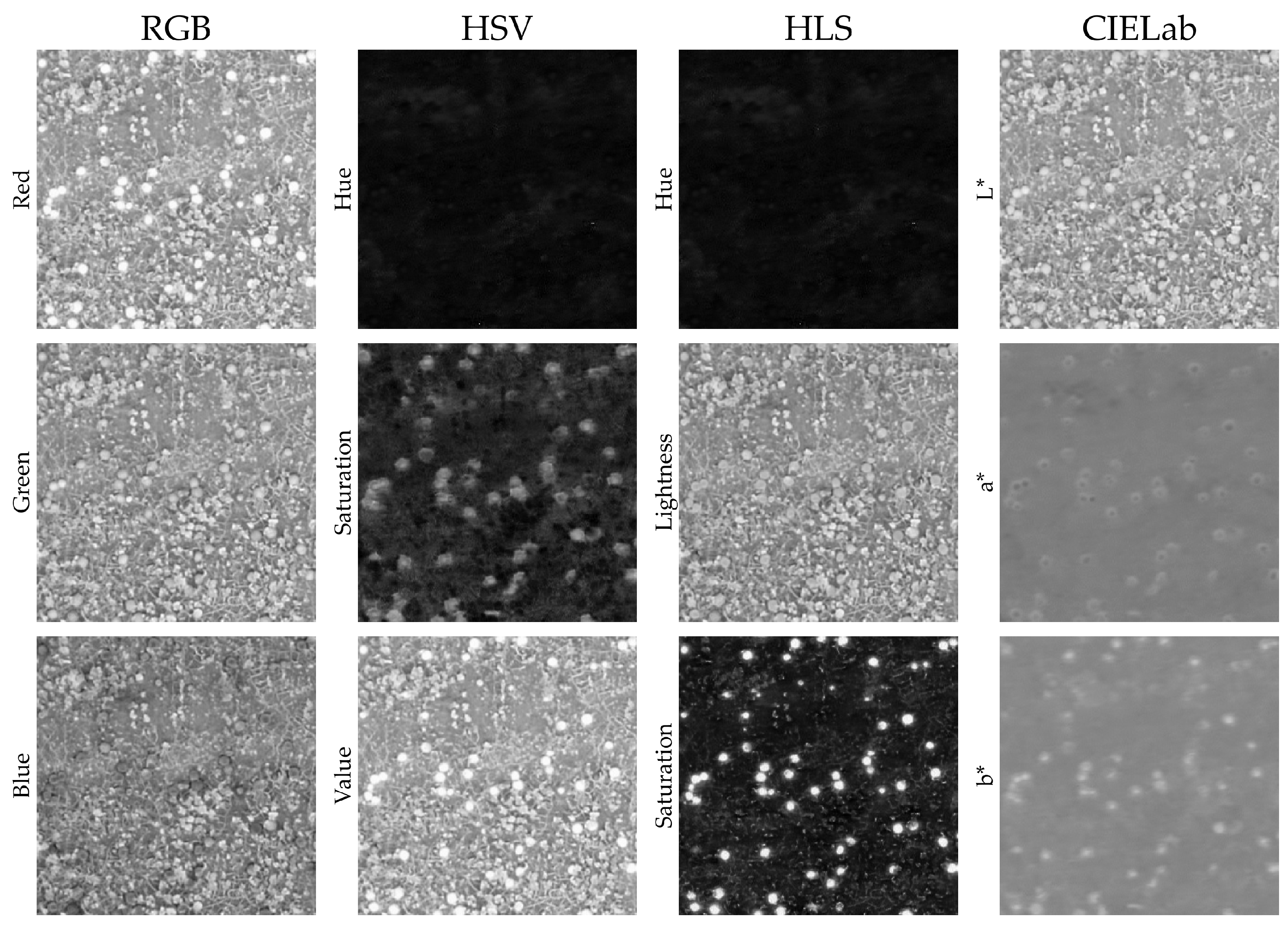
Most common color spaces, RGB (red, green, and blue), HSV (hue, saturation, and value), HLS (hue, lightness, and saturation), and CIELab (L*, a*, and b*), were tested to choose the most applicable. Multiple randomly chosen tiles were examined. In Figure 2, the difference between color spaces is clearly visible. Pumpkins are not clearly visible in all presented bands. There is a perceptible response in the red band of the RGB color space, saturation, and value bands in the HSV color space, the saturation band in the HLS color space, and the b* band in the CIELab color space. Naturally, pumpkins are more discernible in color spaces closer to human perception—HLS and HSV. However, clearly the highest and most differential response is present in the saturation band of the HLS color space. Additionally, the lightness band, which should only be responsible for a change in light in the scene, can be disregarded. Thus, this color space was used in further processing.
2.2.2. Reference Gathering
To be able to detect pumpkins using their distinct color, its model has to be created. For each survey, weather conditions, or pumpkin type, this model can vary. Consequently, a new model has to be created for each survey encompassing pumpkins from different areas of the field.
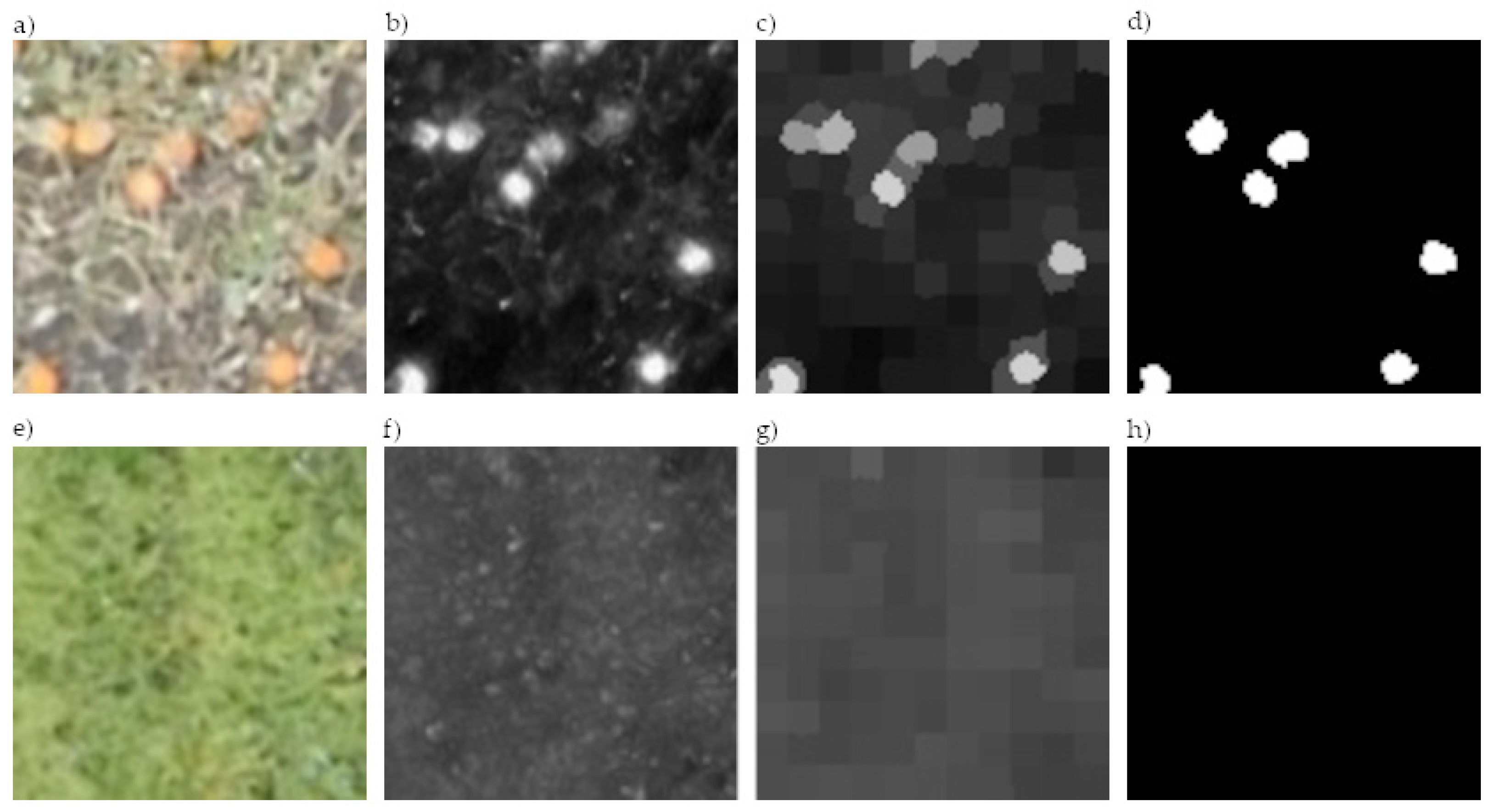
Pumpkins’ natural high response in the saturation band of HLS color space is used here, as the difference between background and pumpkin objects is utmost in this band (Figure 2). A whole orthomosaic is divided into 2.5 × 2.5 m squares. Then, a random set of 30 tiles are chosen (Figure 3a,e), where for the saturation band a clustering process is conducted (Figure 3b,f) [22]. Superpixel creation is tailored to the typical size of a pumpkin and the size of the tile.
The tile is thus divided into n superpixels with a high level of compactness (Figure 3c,g). If a pumpkin is not present, the superpixels have a tendency to form a square. Then, each superpixel is evaluated against statistics of the whole tile. To be classified as a pumpkin, its mean saturation value has to be higher than the median saturation value (assumed value of the background) plus threshold_r standard deviations of the whole tile (Figure 3d,h).
All pixels from all the pumpkin clusters from all chosen tiles form a basis to calculate reference color and reference covariance for the hue and saturation bands in the HLS color space. It is worth noting that not all pumpkins are chosen within the tile, as their size might be too small. Moreover, other objects can have high saturation and be selected. However, when multiple tiles are taken into consideration, the overwhelming majority of selected superpixels should be pumpkins; thus, after calculating its statistics, the influence of other objects should be minimal.
Next, chosen reference tiles are processed again to establish a threshold for further processing. When examining typical color values for pumpkin pixels, the hue and saturation values are observed to follow a multivariate normal distribution, with a low covariance between the hue and saturation values. As the variance in the saturation band is much larger (around 60 times) than the variance in the hue band, a distance metric that takes that into account is needed. Thus, Mahalanobis distance was chosen as a suitable distance metric [23]. The Mahalanobis distance is defined as:
where is the color value of the pixel to segment and and S describe the pumpkin color distribution in terms of the average color value and the associated covariance matrix. Then, summary statistics of the calculated Mahalanobis distances were calculated—mean and standard deviation. The threshold for further segmentation was chosen as a mean plus threshold_m standard deviations.
2.2.3. Segmenting Orthomosaics
For each pixel in the orthomosaic, the Mahalanobis distance to the pumpkin color model was calculated. The generated distance image was then thresholded. Pixels with a distance smaller than the threshold value were considered to originate from pumpkin objects, while the remaining pixels were marked as background.
To reduce noise from the color segmentation, two filters were applied to the segmented image, first median blur with threshold_mb × threshold_mb pixels operating window and then a dilatation with a square kernel of threshold_d × threshold_d pixels.
2.2.4. Counting Pumpkins
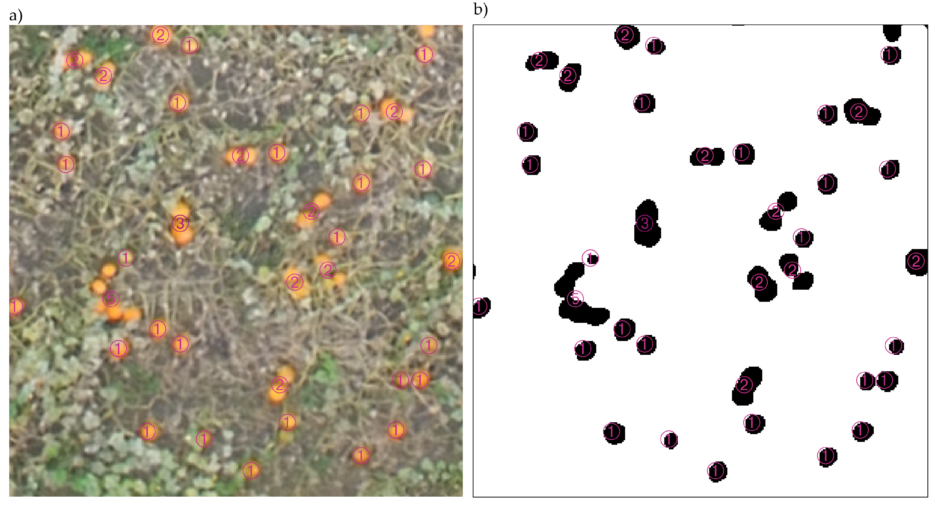
The area and eccentricity of all the detected blobs were calculated. Then, assuming that the majority of detected blobs contain one pumpkin, the median size and standard deviation were calculated for all blobs in the orthomosaic. To detect blobs with multiple pumpkins (Figure 4b), a threshold was set as median pumpkin size plus threshold_a standard deviation. In all the blobs bigger than that, the number of pumpkins in each blob was approximated through the following relation:
where area is the area of the blob and is the median area of blobs which appear to contain exactly one pumpkin.
3. Results
3.1. Threshold Sensitivity Analysis
All chosen thresholds within the algorithm were subjected to threshold sensitivity analysis based on the G2017_102-1 dataset. This includes:
- Number of superpixels and conciseness parameter;
- Threshold_r—multiplication of standard deviations to classify superpixels as pumpkins;
- Threshold_m—multiplication of standard deviations for a threshold for Mahalanobis distance segmentation;
- Threshold_mb and threshold_d—kernel sizes for median blur and dilatation operations;
- Threshold_a—multiplication of standard deviations to differentiate between single and multiple pumpkin blobs.
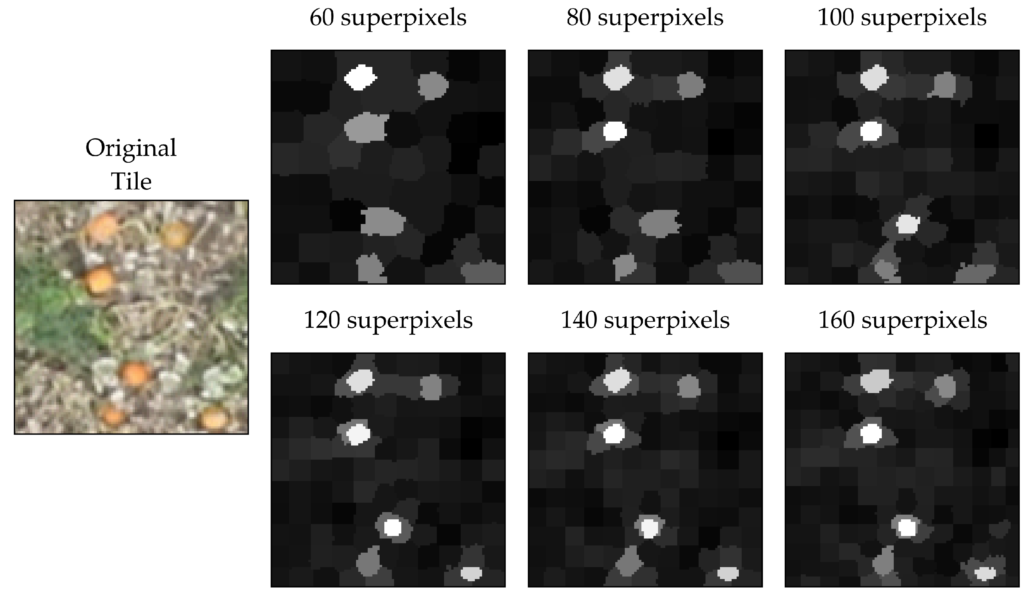
Superpixel creation relies on two parameters: desired number of superpixels and conciseness. Those parameters were chosen to reflect pumpkin size and shape. Since the shape of a pumpkin is round, the conciseness parameter was chosen appropriately, so that the superpixel shape would tend to follow a circular shape. Pumpkin varieties grown within surveyed fields have a diameter of approximately 25 cm. Taking into consideration acquisition blur and background vegetation, a desired size of a superpixel is around 20 cm, then, in a tile of 2.5 × 2.5 m, about 121 of those would fit. Nonetheless, the approach was tested on multiple randomly chosen tiles within different threshold values.
The thresholds 60, 80, 100, 120, 140, and 160 were tested (Figure 5). A visible improvement in segmentation can be seen up till the 120 superpixels threshold, and thus this threshold was chosen for processing.
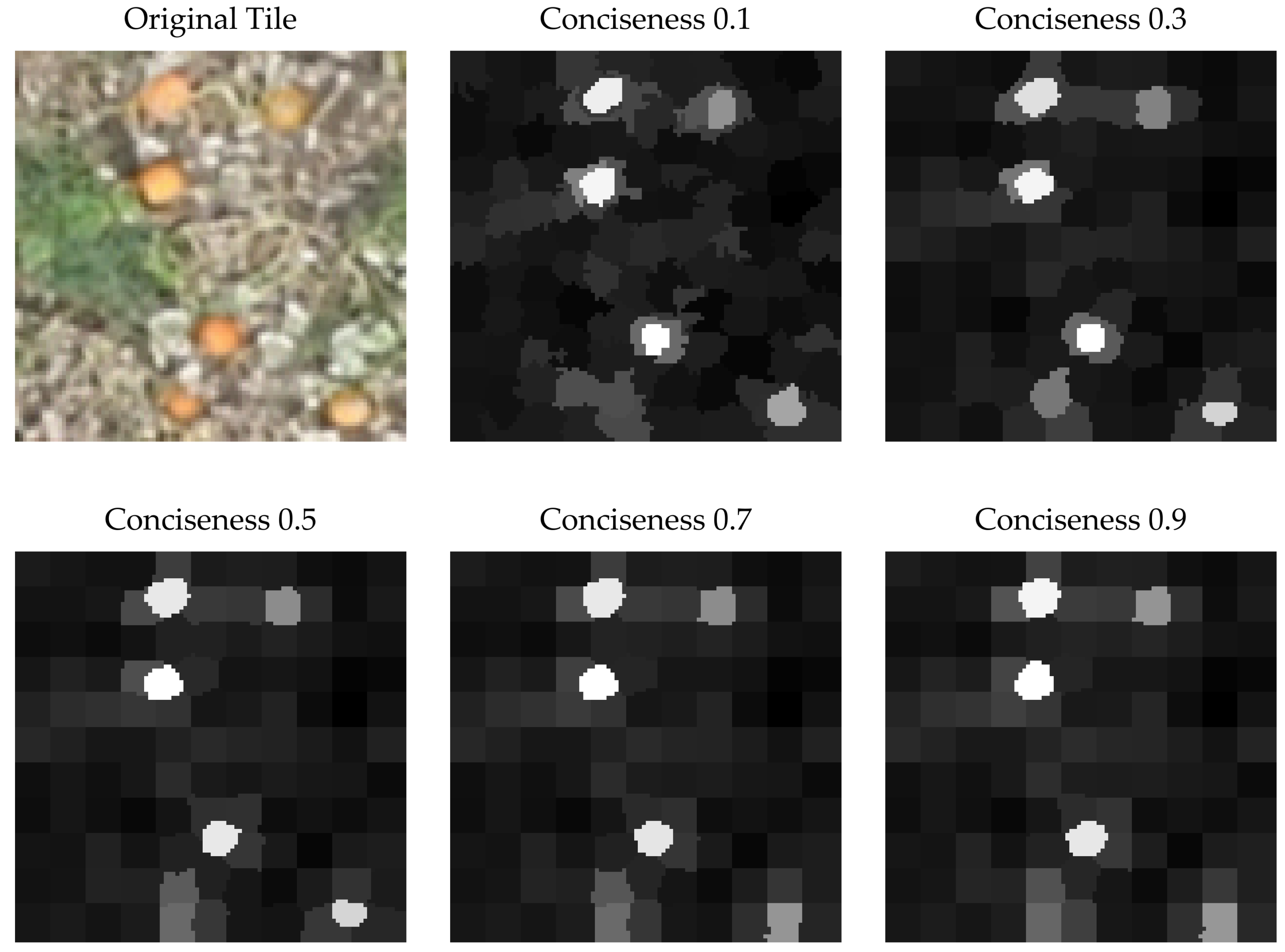
The conciseness parameter depends on the desired shape as well as the number of bands considered in segmentation. The values range between 0 and 100, however, for one band, the values are typically set within the lower side of this spectrum. The values of 0.1, 0.3, 0.5, 0.7, and 0.9 were tested (Figure 6). Following analysis of the results, a threshold of 0.3 was chosen as the optimal solution for detail in color and roundness of the superpixels.
Pumpkin segmentation threshold differentiates between pumpkins and background in the reference-gathering stage and is dependent on parameter threshold_r. Due to superpixel size or vegetation obstacles, not all pumpkin superpixels contain a clear pumpkin image. What is needed is reference pumpkin color, thus, the reference pixel set should be as clear as possible. Consequently, more important in this process is limiting false positive detection than false negative.
A set of randomly chosen reference tiles was subjected to the thresholding process using threshold_r values 1.5, 2, 2.5, 3, 3.5, and 4. The results were compared by looking for false positives. Figure 7 presents the results for selected reference tiles. It is clearly visible that improvement stagnates around the threshold_r of 2.5 standard deviations. However, there is still one false positive present. A threshold_r of three standard deviations is more restrictive but should keep the results clean.
Segmentation on the basis of the Mahalanobis distance requires a cut point threshold. The threshold is established using the mean and standard deviation of the Mahalanobis distance for pumpkin pixels in the reference gathering stage. Still, the multiplication parameter threshold_m needs to be established. The values 0.5, 1.0, 1.5, 2.0, and 2.5 were tested. As visible in Figure 8, the threshold value of 0.5 is too limited, however, the 1.5 threshold value provides no new true positive objects, but a lot of noise and false negatives. This only escalates in higher thresholds. As a consequence, threshold_m equal to 1 was chosen.
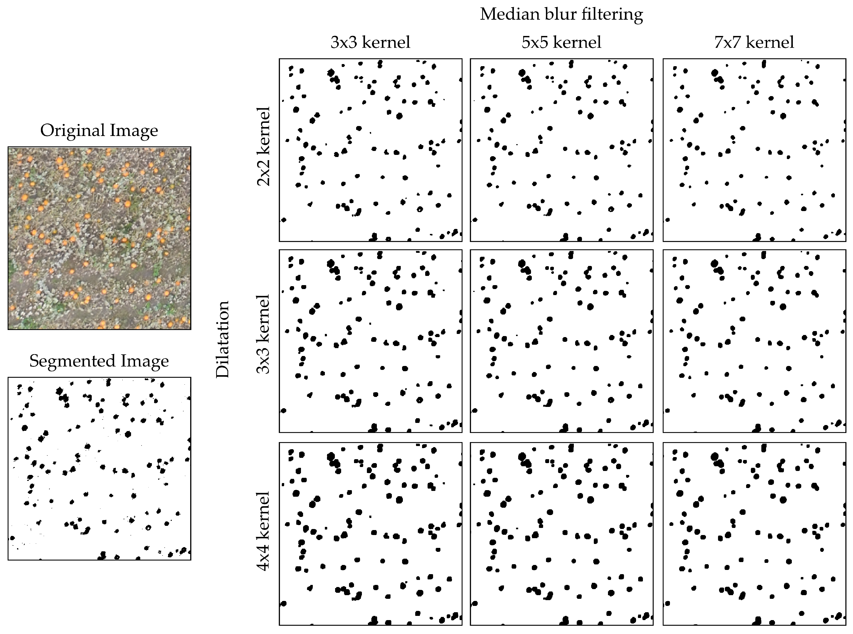
Cleaning up the noise in the segmented image was performed by using two morphological operations—median blur and dilatation. The kernel sizes for both operations were tested at the same time. For median blur values of 3 × 3, 5 × 5, and 7 × 7, mask sizes were tested. For dilatation, kernels of 2 × 2, 3 × 3, and 4 × 4 were tested. There is not much variation in the resultant images (Figure 9), however, threshold_mb = 5 and threshold_md = 3 seem to be simultaneously removing the noise, while not overly enlarging objects.
The last threshold used in the proposed algorithm differentiates between single and multiple pumpkin blobs. Multiple values were tested to establish the correct threshold. 16 randomly chosen 10 × 10 m tiles were analyzed looking for errors, where a single pumpkin was classified as multiple pumpkins, or multiple pumpkins were classified as a single one. The results are presented in Figure 10. As seen in the results, minimum values of errors are achieved for threshold_a values 1.1–1.4, with a definite minimum in 1.2.
3.2. Results
All datasets were processed on a HP laptop with Intel® Core™ i7-8650U CPU @ 1.90 GHz × 8 processor, 16GB RAM, and Intel® UHD Graphics 620. Processing parameters for all the datasets are in Table 2 and results are in Table 3.
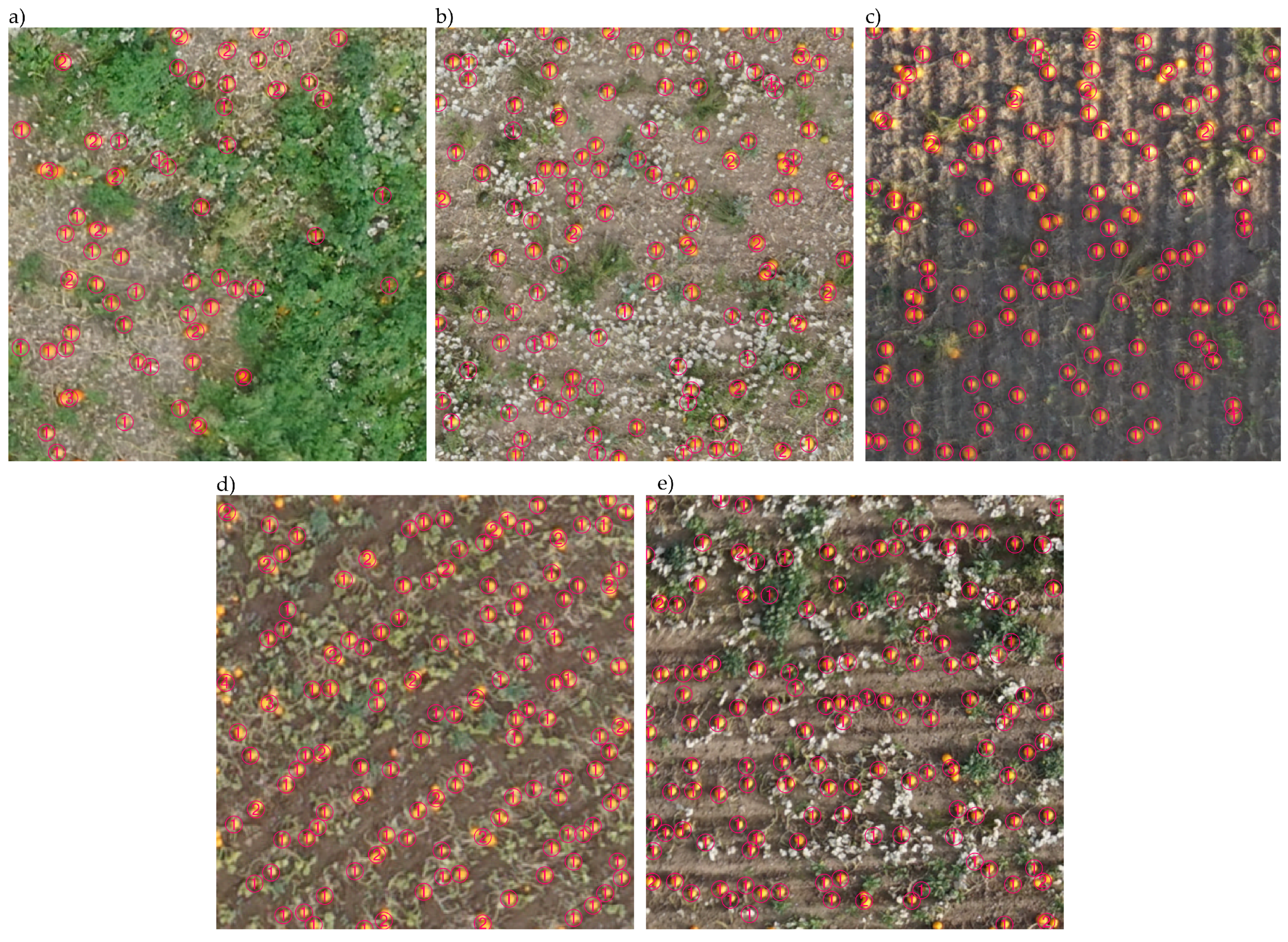
Visual check of the data showed that the majority of the pumpkins were detected correctly in all the datasets (Figure 11). Particularly interesting are results from field 105-0 in 2020. The survey was conducted twice on the field, with a 3 week time difference as well as GSD difference. The importance of correct timing is very visible here. Almost 70,000 more pumpkins were detected in the later orthomosaic. It is possible that GSD size had an influence here, as it was significantly smaller. However, most likely the plant’s leaves have not shrunk yet, and so a significant amount of pumpkins are not visible in the imagery (Figure 12).
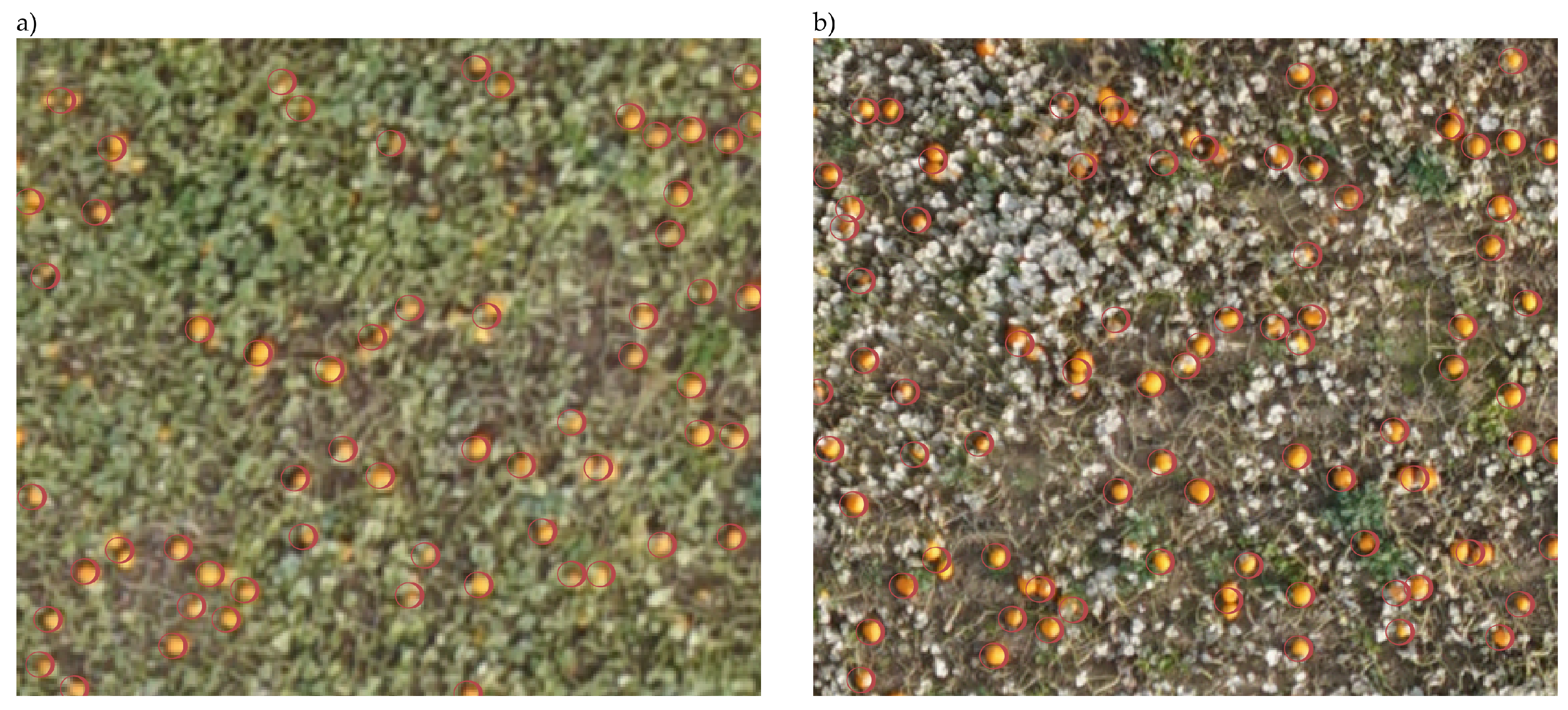
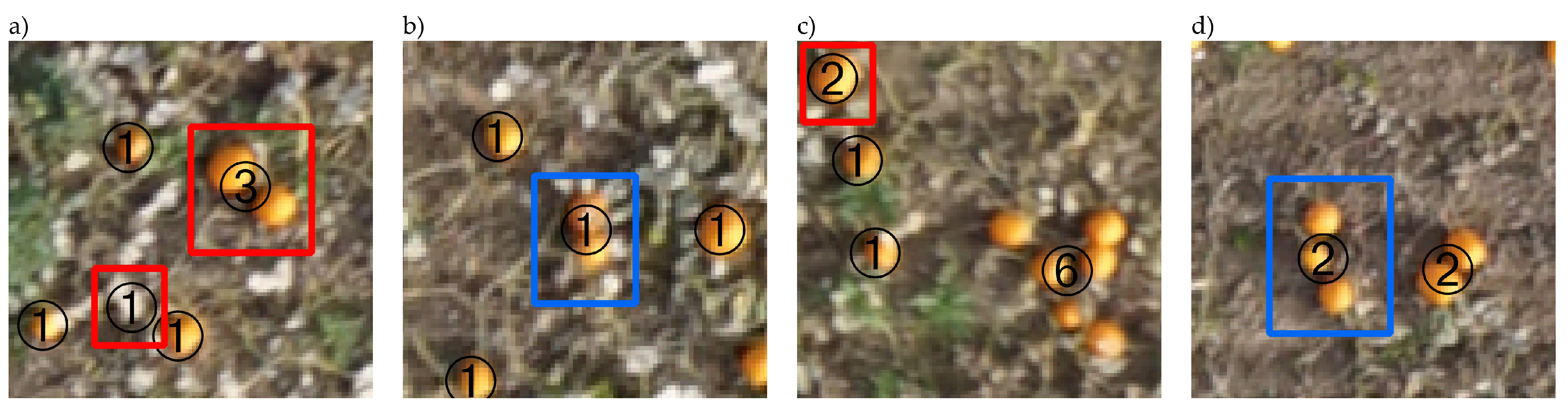
To validate the results, 5% of the area of each orthomosaic was processed manually in 10 × 10 m randomly chosen tiles. All pumpkins were counted and false positives and false negatives were noted. All not-labeled pumpkins, or pumpkin blobs that counted fewer than the actual pumpkin number, were labeled as false negatives (Figure 13b,d). Elements of the background or pumpkin blobs showing more than the actual number of the pumpkins were labeled as false positives (Figure 13a,c). Next Precision, Recall, and F1 score were calculated (Table 4).
3.3. Discussion
The results are very good. Both precision and recall achieve very high values, with the lowest score being 0.959. This means that almost all of the pumpkins are counted and not many are disregarded or falsely detected.
A similar accuracy was obtained by [9]; their approach was based on manual annotation of pumpkin pixels compared with the automatic method described in this paper. However, even comparing with a very different counting task (rapeseed stands), the algorithm error rate is much lower than the 5% error reported by [17].
A simple algorithm based on k-means clustering for choosing a segmentation threshold was introduced by [7] to locate maize tassels in red-edge images. Our more involved algorithm for sampling of pumpkin-colored pixels was implemented and tested on a single dataset but was seen to perform extremely well on all of the five tested datasets.
The number of counted pumpkins might not translate directly to the field yield. With the GSD of this size, there is no way to judge if the pumpkin is damaged in any way. Rotten or mechanically damaged fruit is still counted. That also applies to very small pumpkins. A size limit could be introduced, but the size of the blob is not always representative of the true pumpkin size, as the fruit can be obscured by leaves or other objects. Thus, the results should be treated as overestimation.
4. Conclusions
UAV images can be used to estimate the yield of pumpkin fields accurately to assist farmers in optimizing their sales. The algorithm is fully automated and robust. However, it is required to go out and acquire drone footage at the proper growth stage to be able to count the pumpkins reliably. This relies on particular properties of pumpkins—both color and size, though none of them provide hard thresholds.
The use of hue and saturation from the HLS color space ensures the detection of pumpkins in various lighting conditions. Algorithm performance has been thoroughly tested, showing high performance in all datasets. The lowest F1 score (0.970) for the validation process shows the high efficiency and precision of the method.
The dependency of the algorithm’s performance using the selected intuitive thresholds have also been investigated. Slight changes in parameters do not change the outcome significantly.
Author Contributions
Conceptualization, H.S.M.; methodology, H.S.M. and E.P.; software, H.S.M. and E.P.; validation, E.P.; resources, H.S.M.; data curation, E.P.; writing—original draft preparation, H.S.M. and E.P.; writing—review and editing, H.S.M. and E.P.; visualization, E.P.; funding acquisition, H.S.M. All authors have read and agreed to the published version of the manuscript.
Funding
This project was funded by the Development Fund of EnergiFyn, Denmark.
Acknowledgments
We want to thank Gyldensteen Manor for providing access to their fields and their know-how about growing pumpkins.
Conflicts of Interest
The authors declare no conflict of interest.
References
- Floreano, D.; Wood, R.J. Science, technology and the future of small autonomous drones. Nature 2015, 521, 460–466. [Google Scholar] [CrossRef] [PubMed] [Green Version]
- Shi, Y.; Thomasson, J.A.; Murray, S.C.; Pugh, N.A.; Rooney, W.L.; Shafian, S.; Rajan, N.; Rouze, G.; Morgan, C.L.S.; Neely, H.L.; et al. Unmanned Aerial Vehicles for High-Throughput Phenotyping and Agronomic Research. PLoS ONE 2016, 11, e0159781. [Google Scholar] [CrossRef] [PubMed] [Green Version]
- He, L.; Fang, W.; Zhao, G.; Wu, Z.; Fu, L.; Li, R.; Majeed, Y.; Dhupia, J. Fruit yield prediction and estimation in orchards: A state-of-the-art comprehensive review for both direct and indirect methods. Comput. Electron. Agric. 2022, 195, 106812. [Google Scholar] [CrossRef]
- Sankaran, S.; Quirós, J.J.; Knowles, N.R.; Knowles, L.O. High-Resolution Aerial Imaging Based Estimation of Crop Emergence in Potatoes. Am. J. Potato Res. 2017, 94, 658–663. [Google Scholar] [CrossRef]
- Chen, R.; Chu, T.; Landivar, J.A.; Yang, C.; Maeda, M.M. Monitoring cotton (Gossypium hirsutum L.) germination using ultrahigh-resolution UAS images. Precis. Agric. 2018, 19, 161–177. [Google Scholar] [CrossRef]
- Varela, S.; Dhodda, P.; Hsu, W.; Prasad, P.V.; Assefa, Y.; Peralta, N.; Griffin, T.; Sharda, A.; Ferguson, A.; Ciampitti, I. Early-Season Stand Count Determination in Corn via Integration of Imagery from Unmanned Aerial Systems (UAS) and Supervised Learning Techniques. Remote Sens. 2018, 10, 343. [Google Scholar] [CrossRef] [Green Version]
- Kumar, A.; Desai, S.V.; Balasubramanian, V.N.; Rajalakshmi, P.; Guo, W.; Balaji Naik, B.; Balram, M.; Desai, U.B. Efficient Maize Tassel-Detection Method using UAV based remote sensing. Remote Sens. Appl. Soc. Environ. 2021, 23, 100549. [Google Scholar] [CrossRef]
- Li, B.; Xu, X.; Han, J.; Zhang, L.; Bian, C.; Jin, L.; Liu, J. The estimation of crop emergence in potatoes by UAV RGB imagery. Plant Methods 2019, 15, 15. [Google Scholar] [CrossRef] [PubMed] [Green Version]
- Wittstruck, L.; Kühling, I.; Trautz, D.; Kohlbrecher, M.; Jarmer, T. UAV-Based RGB Imagery for Hokkaido Pumpkin (Cucurbita max.) Detection and Yield Estimation. Sensors 2020, 21, 118. [Google Scholar] [CrossRef] [PubMed]
- Jin, X.; Liu, S.; Baret, F.; Hemerlé, M.; Comar, A. Estimates of plant density of wheat crops at emergence from very low altitude UAV imagery. Remote Sens. Environ. 2017, 198, 105–114. [Google Scholar] [CrossRef] [Green Version]
- Gnädinger, F.; Schmidhalter, U. Digital Counts of Maize Plants by Unmanned Aerial Vehicles (UAVs). Remote Sens. 2017, 9, 544. [Google Scholar] [CrossRef] [Green Version]
- Koh, J.C.; Hayden, M.; Daetwyler, H.; Kant, S. Estimation of crop plant density at early mixed growth stages using UAV imagery. Plant Methods 2019, 15, 64. [Google Scholar] [CrossRef] [PubMed]
- Fernandez-Gallego, J.A.; Lootens, P.; Borra-Serrano, I.; Derycke, V.; Haesaert, G.; Roldán-Ruiz, I.; Araus, J.L.; Kefauver, S.C. Automatic wheat ear counting using machine learning based on RGB UAV imagery. Plant J. 2020, 103, 1603–1613. [Google Scholar] [CrossRef] [PubMed]
- Mekhalfi, M.L.; Nicolò, C.; Ianniello, I.; Calamita, F.; Goller, R.; Barazzuol, M.; Melgani, F. Vision system for automatic on-tree kiwifruit counting and yield estimation. Sensors 2020, 20, 4214. [Google Scholar] [CrossRef] [PubMed]
- Ribera, J.; Chen, Y.; Boomsma, C.; Delp, E.J. Counting plants using deep learning. In Proceedings of the 2017 IEEE Global Conference on Signal and Information Processing (GlobalSIP), Montreal, QC, Canada, 14–16 November 2017; Volume 2018, pp. 1344–1348. [Google Scholar] [CrossRef]
- Valente, J.; Sari, B.; Kooistra, L.; Kramer, H.; Mücher, S.; Kramer, ·.H.; Mücher, ·.S.; Nl, J.V. Automated crop plant counting from very high-resolution aerial imagery. Precis. Agric. 2020. [Google Scholar] [CrossRef]
- Zhang, J.; Zhao, B.; Yang, C.; Shi, Y.; Liao, Q.; Zhou, G.; Wang, C.; Xie, T.; Jiang, Z.; Zhang, D.; et al. Rapeseed Stand Count Estimation at Leaf Development Stages With UAV Imagery and Convolutional Neural Networks. Front. Plant Sci. 2020. [Google Scholar] [CrossRef] [PubMed]
- Vadhavkar, N. Case Study: Identifying Pumpkins with Drones and Machine Learning—Raptor Maps. 2017. Available online: https://deveron.com/wp-content/uploads/2020/01/deveron-casestudy-pumpkin_nov1-1.pdf (accessed on 1 September 2019).
- Agisoft. Metashape. 2018. Available online: www.agisoft.com (accessed on 1 September 2019).
- Bradski, G. The OpenCV Library. Dr. Dobb’s J. Softw. Tools 2000, 25, 120–123. [Google Scholar]
- Gillies, S.; Ward, B.; Petersen, A.S. Rasterio: Geospatial Raster I/O for Python Programmers. 2013. Available online: https//github.com/mapbox/rasterio (accessed on 1 March 2019).
- Achanta, R.; Shaji, A.; Smith, K.; Lucchi, A.; Fua, P.; Süsstrunk, S. SLIC Superpixels Compared to State-of-the-Art Superpixel Methods. IEEE Trans. Pattern Anal. Mach. Intell. 2012, 34, 2274–2282. [Google Scholar] [CrossRef] [PubMed] [Green Version]
- Mahalanobis, P.C. On the generalised distance in statistics. Proc. Natl. Inst. Sci. India 1936, 2, 49–55. [Google Scholar]
- QGIS Geographic Information System. Open Source Geospatial Foundation Project. 2019. Available online: http://www.qgis.org/ (accessed on 10 March 2019).
Figure 1.
Placement of the test fields within Danish boundary (maps available free from kortforsyningen.dk).
Figure 1.
Placement of the test fields within Danish boundary (maps available free from kortforsyningen.dk).

Figure 2.
Randomly selected tile with pumpkins presented in four different color spaces separated by bands.
Figure 2.
Randomly selected tile with pumpkins presented in four different color spaces separated by bands.

Figure 3.
Reference tile with pumpkins (a), its saturation band (b), segmented image (c), and thresholded image (d). Reference tile without pumpkins (e), its saturation band (f), segmented image (g), and thresholded image (h).
Figure 3.
Reference tile with pumpkins (a), its saturation band (b), segmented image (c), and thresholded image (d). Reference tile without pumpkins (e), its saturation band (f), segmented image (g), and thresholded image (h).

Figure 4.
A section of orthomosaic with detected pumpkin blobs and the number of pumpkins they contain visualized (a) and the corresponding thresholded section (b).
Figure 4.
A section of orthomosaic with detected pumpkin blobs and the number of pumpkins they contain visualized (a) and the corresponding thresholded section (b).

Figure 5.
Results of segmentation with different threshold sizes for the number of superpixels.

Figure 6.
Results of segmentation with different conciseness parameter values.

Figure 7.
Results of superpixel segmentation for different values of standard deviation multiplicator—threshold_r.
Figure 7.
Results of superpixel segmentation for different values of standard deviation multiplicator—threshold_r.

Figure 8.
Results of the Mahalanobis distance image being thresholded with different values of threshold_m multiplication.
Figure 8.
Results of the Mahalanobis distance image being thresholded with different values of threshold_m multiplication.

Figure 9.
Results of morphological operations on segmented image for different values of threshold_mb and threshold_d.
Figure 9.
Results of morphological operations on segmented image for different values of threshold_mb and threshold_d.

Figure 10.
Results of pumpkin blob classification for different threshold_a values.

Figure 11.
Sections of processing results for datasets G2017_102-1 (a), G2018_104-0 (b), G2019_106-0 (c), G2020_105-0 I (d), G2020_105-0 II (e).
Figure 11.
Sections of processing results for datasets G2017_102-1 (a), G2018_104-0 (b), G2019_106-0 (c), G2020_105-0 I (d), G2020_105-0 II (e).

Figure 12.
Same section of orthomosaics of field 105-0 for 2020 season 27.08.2020 (a) and 17.09.2020 (b).
Figure 12.
Same section of orthomosaics of field 105-0 for 2020 season 27.08.2020 (a) and 17.09.2020 (b).

Figure 13.
Labeled pumpkin counting errors. False positive in red (a,c) and false negative in blue (b,d).
Figure 13.
Labeled pumpkin counting errors. False positive in red (a,c) and false negative in blue (b,d).


Table 1.
Survey details.
| Dataset | Date | Field | Camera | Area [m2] | GSD [m] |
|---|---|---|---|---|---|
| G2017_102-1 | 19 September 2017 | 102-1 | sensFly S.O.D.A. | 32,066 | 0.025 |
| G2018_104-0 | 23 August 2018 | 104-0 | Sony UMC-R10C | 361,049 | 0.020 |
| G2019_106-0 | 17 September 2019 | 106-0 | Sony UMC-R10C | 229,609 | 0.025 |
| G2020_105-0 I | 27 August 2020 | 105-0 | Sony UMC-R10C | 468,805 | 0.036 |
| G2020_105-0 II | 17 September 2020 | 105-0 | Sony UMC-R10C | 468,805 | 0.025 |
Table 2.
Processing parameters for all datasets.
| Dataset | Reference Tile Size [m] | Superpixels/ Conciseness | threshold_r | threshold_m | threshold_mb/ threshold_d | threshold_a |
|---|---|---|---|---|---|---|
| G2017_102-1 | 2.5 × 2.5 | 30 | 120/0.3 | 3 | 5 × 5/3 × 3 | 1.0 |
| G2018_104-0 | 2.5 × 2.5 | 30 | 120/0.3 | 3 | 5 × 5/3 × 3 | 1.0 |
| G2019_106-0 | 2.5 × 2.5 | 30 | 120/0.3 | 3 | 5 × 5/3 × 3 | 1.0 |
| G2020_105-0 I | 2.5 × 2.5 | 30 | 120/0.3 | 3 | 5 × 5/3 × 3 | 1.0 |
| G2020_105-0 II | 2.5 × 2.5 | 30 | 120/0.3 | 3 | 5 × 5/3 × 3 | 1.0 |
Table 3.
Numerical results for all datasets.
| Dataset | Mahalanobis Threshold | Estimated Number of Pumpkins | Pumpkins per m2 | Processing Time [s] | Reference Color | Covariance Matrix |
|---|---|---|---|---|---|---|
| G2017_102-1 | 1.97 | 23,931 | 0.75 | 11.2 | [17.17 192.37] | [11.71 15.34] [15.34 2286.79] |
| G2018_104-0 | 1.92 | 319,616 | 0.89 | 133.3 | [18.22 186.06] | [9.79 85.20] [85.20 2135.87] |
| G2019_106-0 | 1.99 | 238,986 | 0.51 | 71.1 | [19.16 206.54] | [25.48 131.84] [131.84 1668.06] |
| G2020_105-0 I | 1.98 | 405,826 | 0.87 | 151.0 | [18.46 185.15] | [8.61 41.46] [41.46 2031.58] |
| G2020_105-0 II | 1.94 | 470,685 | 1.00 | 61.5 | [17.94 193.20] | [18.70 124.87] [124.87 1902.46] |
Table 4.
Validation results for all datasets.
| Dataset | Validation Area in 10 × 10 m2 Tiles | True Positive | False Positive | False Negative | Precision | Recall | F1 Score |
|---|---|---|---|---|---|---|---|
| G2017_102-1 | 16 | 1061 | 31 | 32 | 0.972 | 0.971 | 0.971 |
| G2018_104-0 | 181 | 15,297 | 284 | 196 | 0.982 | 0.987 | 0.985 |
| G2019_106-0 | 115 | 11,186 | 479 | 223 | 0.959 | 0.980 | 0.970 |
| G2020_105-0 I | 234 | 20,534 | 84 | 408 | 0.996 | 0.981 | 0.988 |
| G2020_105-0 II | 234 | 21,039 | 271 | 297 | 0.987 | 0.986 | 0.987 |
Publisher’s Note: MDPI stays neutral with regard to jurisdictional claims in published maps and institutional affiliations. |
© 2022 by the authors. Licensee MDPI, Basel, Switzerland. This article is an open access article distributed under the terms and conditions of the Creative Commons Attribution (CC BY) license (https://creativecommons.org/licenses/by/4.0/).
Share and Cite
MDPI and ACS Style
Midtiby, H.S.; Pastucha, E. Pumpkin Yield Estimation Using Images from a UAV. Agronomy 2022, 12, 964. https://0-doi-org.brum.beds.ac.uk/10.3390/agronomy12040964
AMA Style
Midtiby HS, Pastucha E. Pumpkin Yield Estimation Using Images from a UAV. Agronomy. 2022; 12(4):964. https://0-doi-org.brum.beds.ac.uk/10.3390/agronomy12040964
Chicago/Turabian StyleMidtiby, Henrik Skov, and Elżbieta Pastucha. 2022. "Pumpkin Yield Estimation Using Images from a UAV" Agronomy 12, no. 4: 964. https://0-doi-org.brum.beds.ac.uk/10.3390/agronomy12040964
Note that from the first issue of 2016, this journal uses article numbers instead of page numbers. See further details here.