Soil Moisture Mapping Using Multi-Frequency and Multi-Coil Electromagnetic Induction Sensors on Managed Podzols


Abstract
:1. Introduction
2. Materials and Method
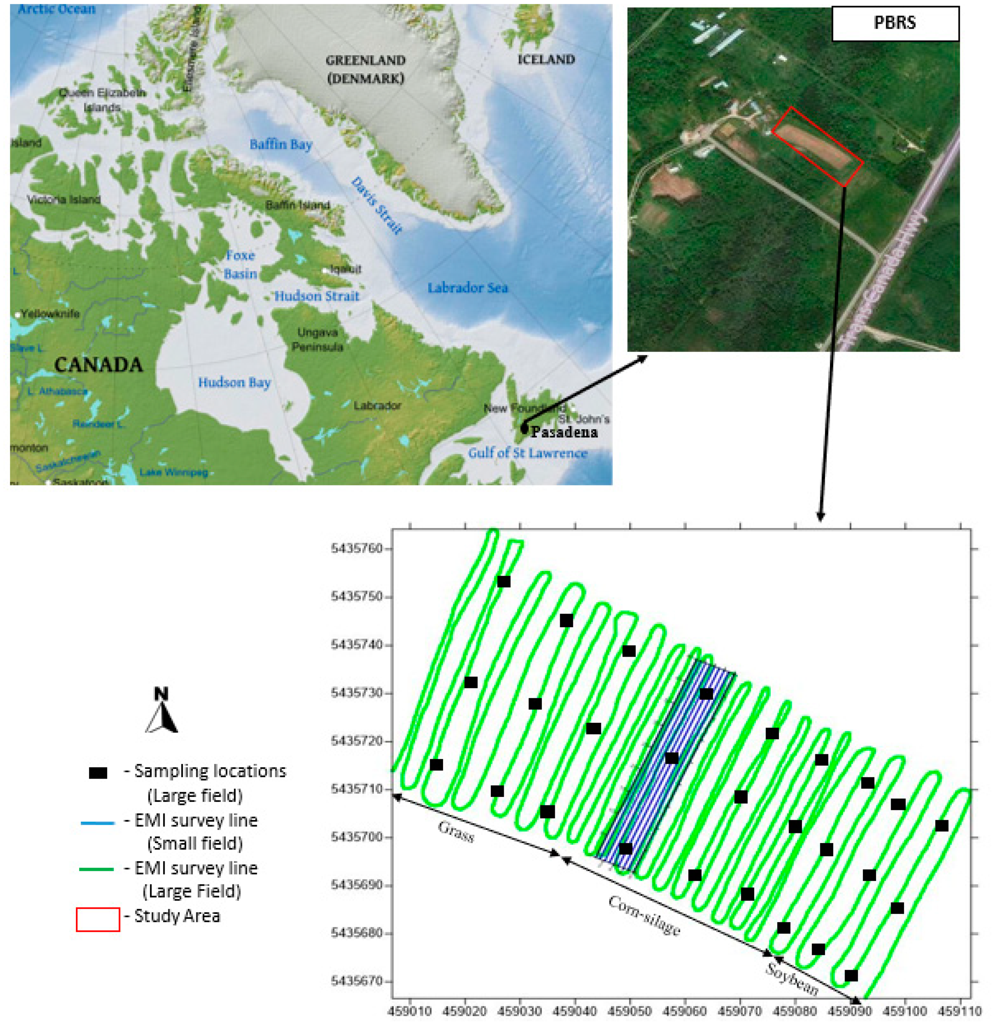
2.1. Study Site
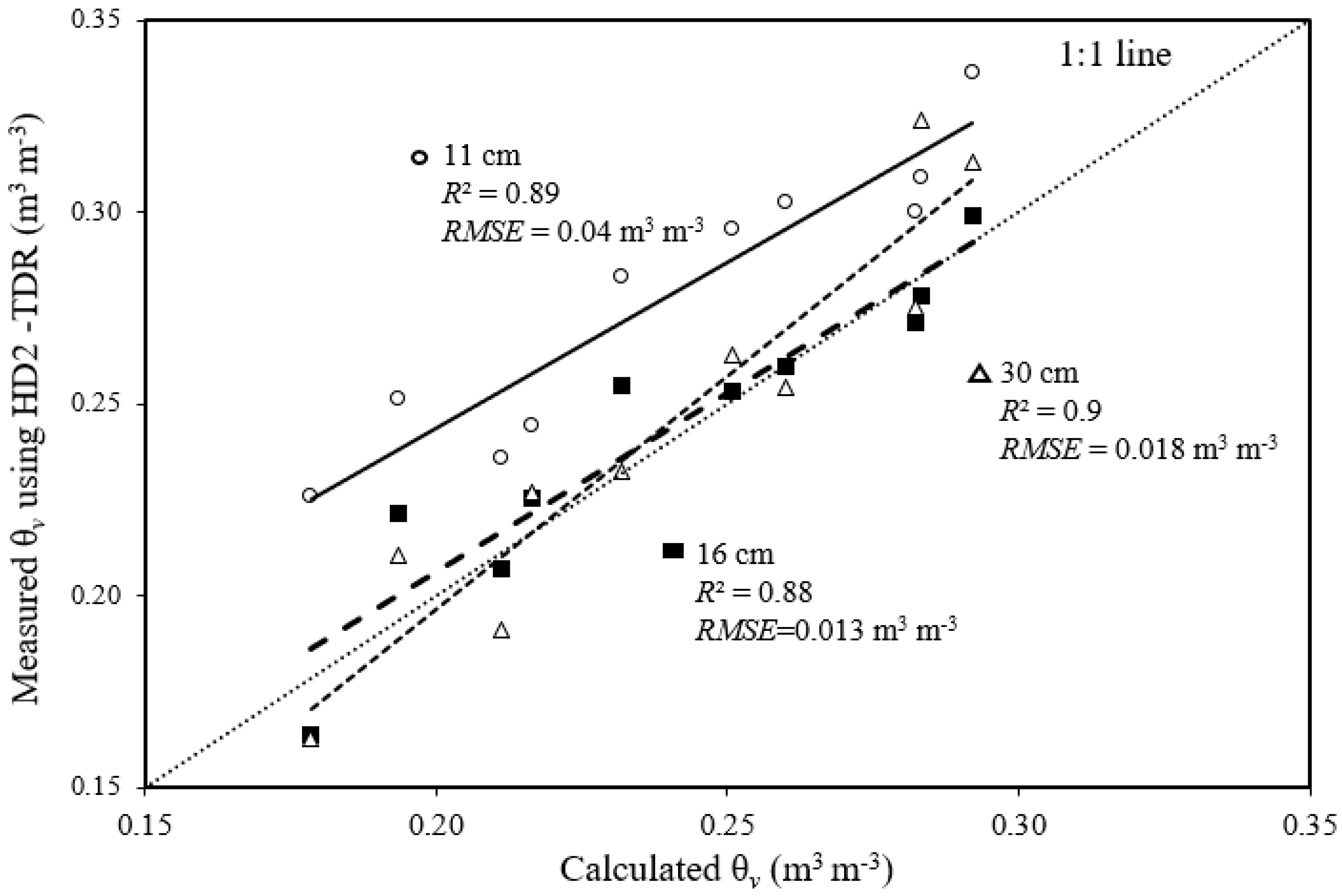
2.2. SMC Data Recording and TDR Calibration
2.3. EMI Survey
2.4. Field Calibration and Validation
2.5. Soil Sampling
2.6. Data Analysis
3. Results
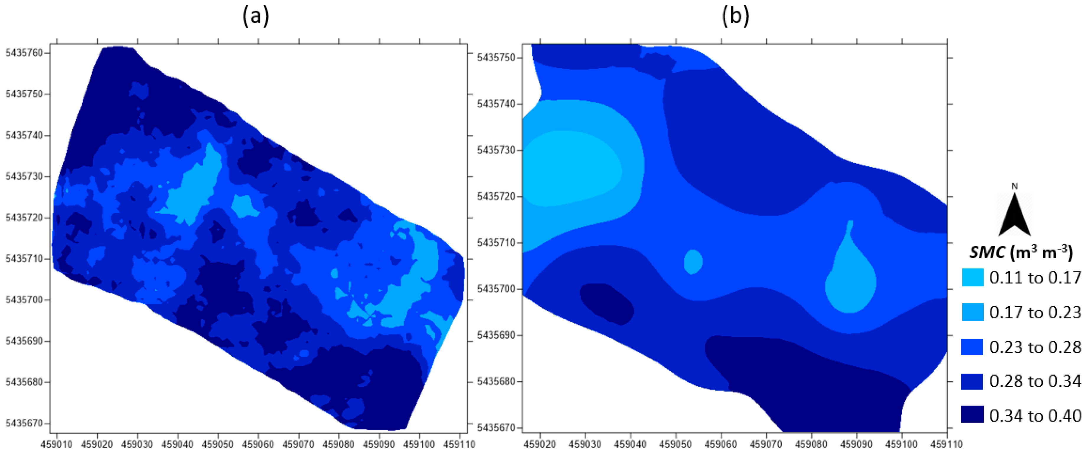
3.1. SMC Results
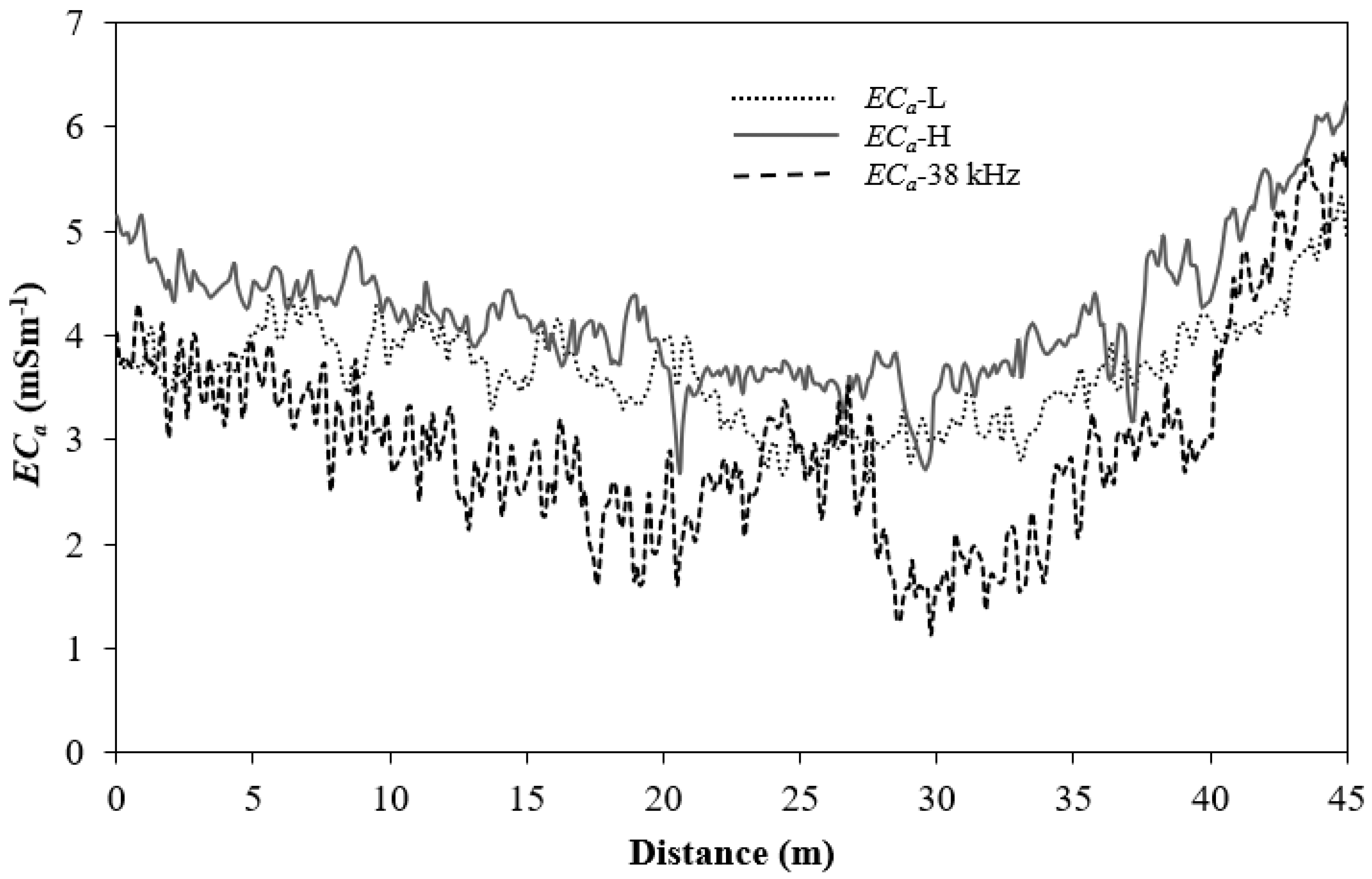
3.2. EMI Results
3.3. Basic Statistics
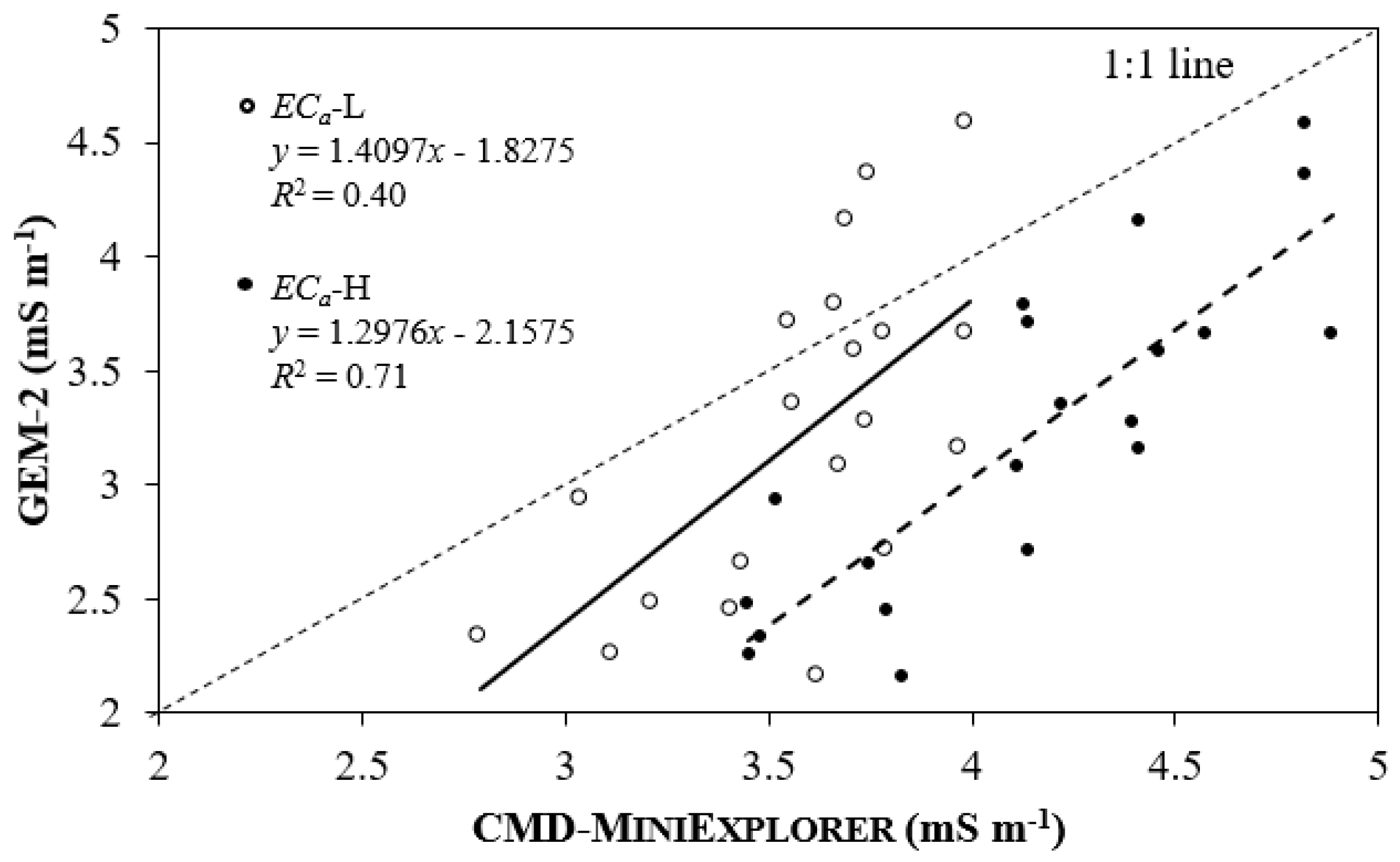
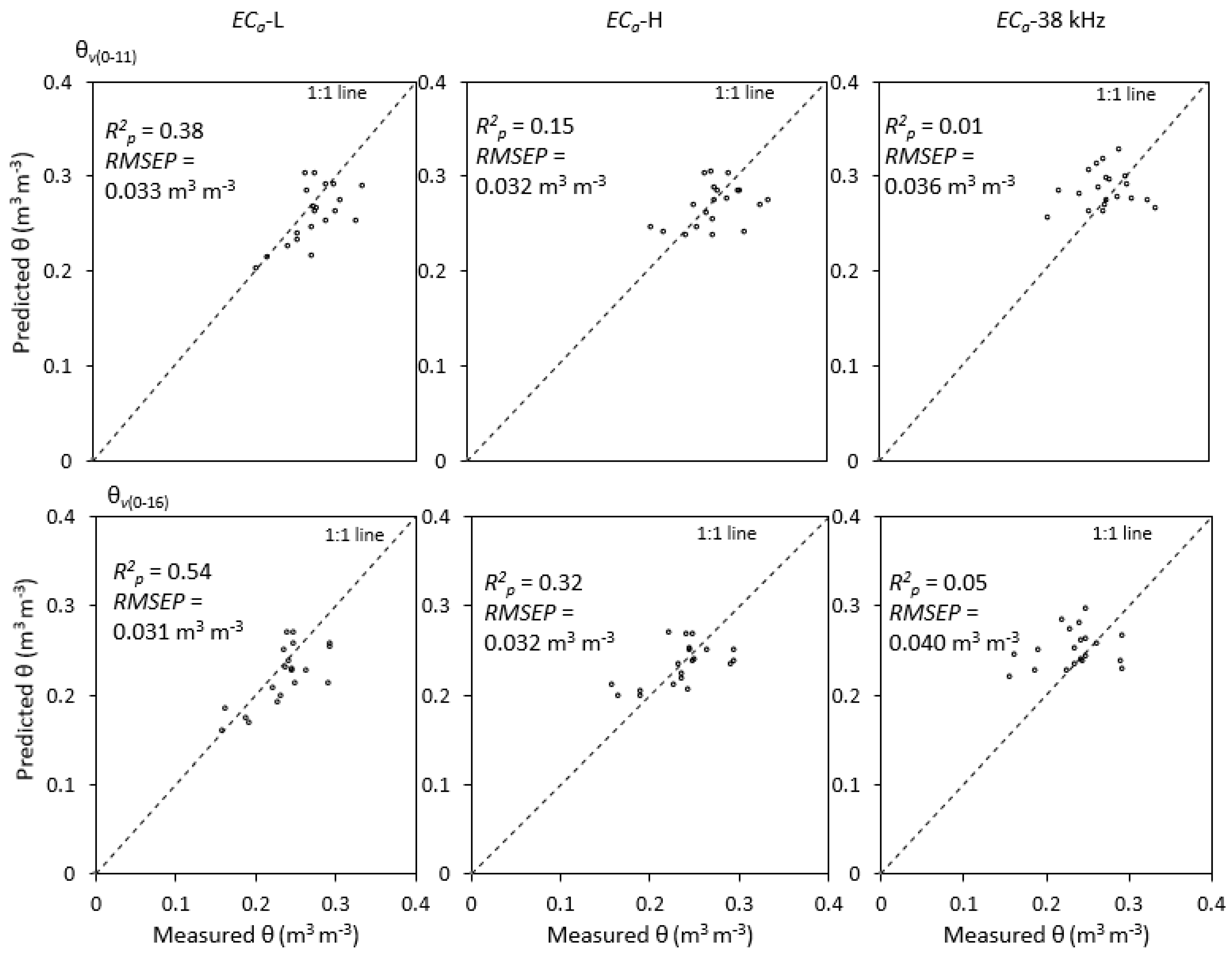
3.4. Regression Analysis
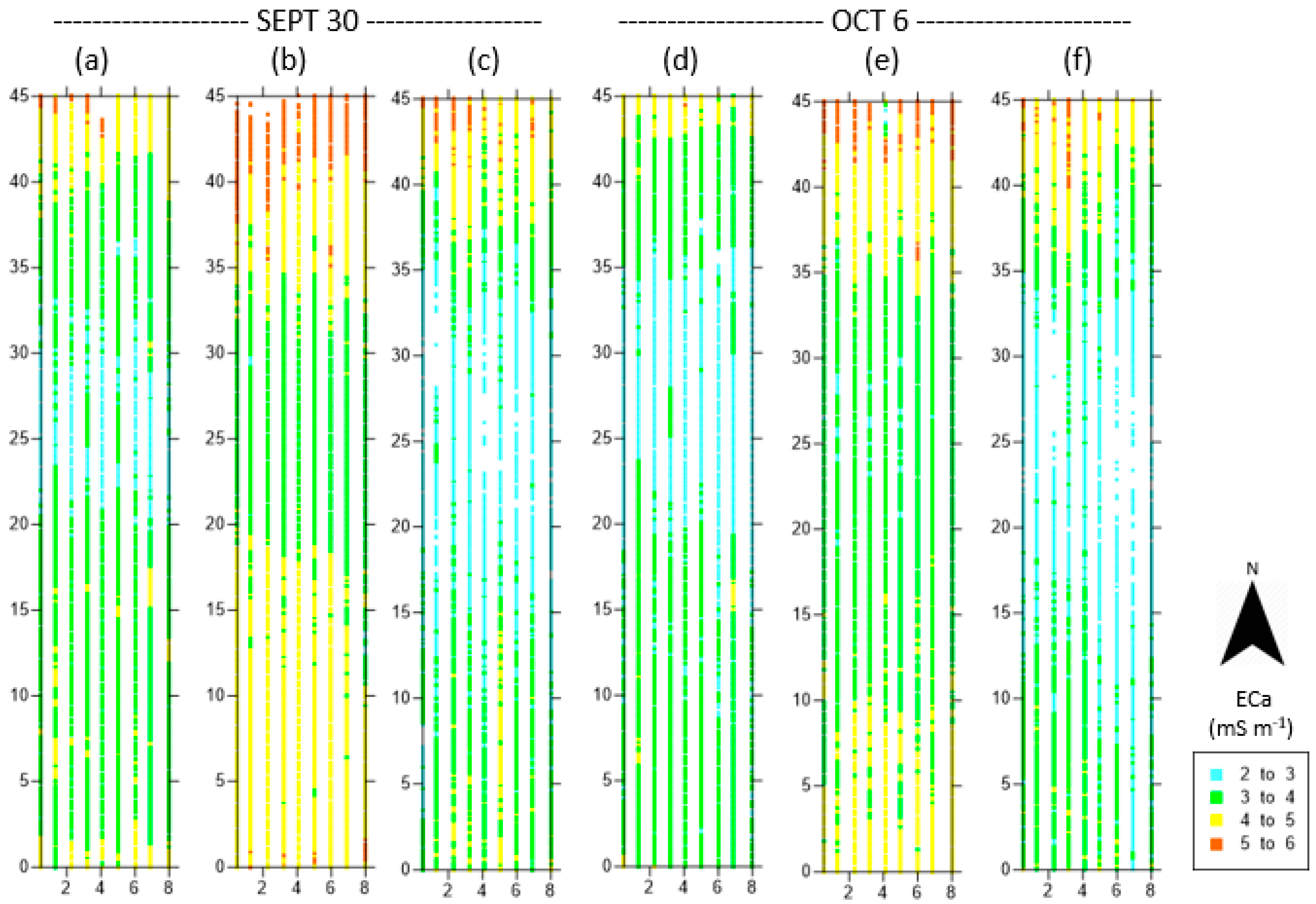
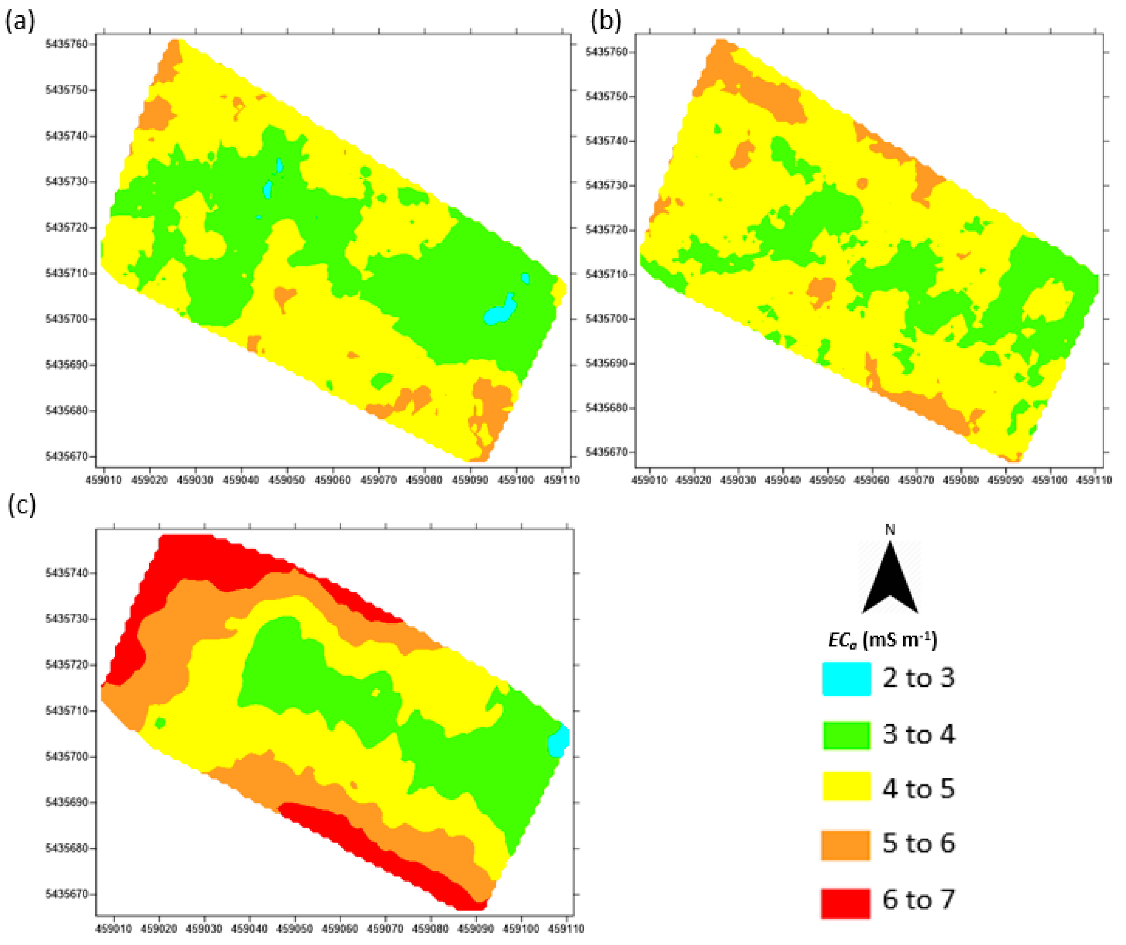
3.5. ECa Mapping
4. Discussion
5. Conclusions
Author Contributions
Funding
Acknowledgments
Conflicts of Interest
References
- Corwin, D.L.; Lesch, S.M. Characterizing soil spatial variability with apparent soil electrical conductivity part II. case study. Comput. Electron. Agric. 2005, 46, 135–152. [Google Scholar] [CrossRef]
- Peralta, N.R.; Costa, J.L. Delineation of management zones with soil apparent electrical conductivity to improve nutrient management. Comput. Electron. Agric. 2013, 99, 218–226. [Google Scholar] [CrossRef] [Green Version]
- Lesch, S.M.; Corwin, D.L.; Robinson, D.A. Apparent soil electrical conductivity mapping as an agricultural management tool in arid zone soils. Comput. Electron. Agric. 2005, 46, 351–378. [Google Scholar] [CrossRef] [Green Version]
- Bongiovanni, R.; Lowenberg-DeBoer, J. Precision agriculture and sustainability. Precis. Agric. 2004, 5, 359–387. [Google Scholar] [CrossRef]
- Kyaw, T.; Ferguson, R.B.; Adamchuk, V.I.; Marx, D.B.; Tarkalson, D.D.; McCallister, D.L. Delineating site-specific management zones for pH-induced iron chlorosis. Precis. Agric. 2008, 9, 71–84. [Google Scholar] [CrossRef] [Green Version]
- Fortes, R.; Millán, S.; Prieto, M.H.; Campillo, C. A methodology based on apparent electrical conductivity and guided soil samples to improve irrigation zoning. Precis. Agric. 2015, 16, 441–454. [Google Scholar] [CrossRef]
- Corwin, D.L.; Lesch, S.M. Apparent soil electrical conductivity measurements in agriculture. Comput. Electron. Agric. 2005, 46, 11–43. [Google Scholar] [CrossRef]
- Doolittle, J.A.; Brevik, E.C. The use of electromagnetic induction techniques in soils studies. Geoderma 2014, 223, 33–45. [Google Scholar] [CrossRef] [Green Version]
- Galagedara, L.W.; Parkin, G.W.; Redman, J.D.; von Bertoldi, P.; Endres, A.L. Field studies of the GPR ground wave method for estimating soil water content during irrigation and drainage. J. Hydrol. 2005, 301, 182–197. [Google Scholar] [CrossRef]
- Wijewardana, Y.G.N.S.; Galagedara, L.W. Estimation of spatio-temporal variability of soil water content in agricultural fields with ground penetrating radar. J. Hydrol. 2010, 391, 24–33. [Google Scholar] [CrossRef]
- Topp, G.C.; Davis, J.L.; Annan, A.P. Electromagnetic determination of soil water content: Measurements in coaxial transmission lines. Water Resour. Res. 1980, 16, 574–582. [Google Scholar] [CrossRef]
- Ferré, P.A.; Redman, J.D.; Rudolph, D.L.; Kachanoski, R.G. The dependence of the electrical conductivity measured by time domain reflectometry on the water content of a sand. Water Resour. Res. 1998, 34, 1207–1213. [Google Scholar] [CrossRef] [Green Version]
- Desilets, D.; Zreda, M.; Ferre, T.P.A. Nature’s neutron probe: Land surface hydrology at an elusive scale with cosmic rays. Water Resour. Res. 2010. [Google Scholar] [CrossRef]
- Franz, T.E.; Zreda, M.; Ferre, P.A.; Rosolem, R. An assessment of the effect of horizontal soil moisture heterogeneity on the area-average measurement of cosmic-ray neutrons. Water Resour. Res. 2013, 49, 1–10. [Google Scholar] [CrossRef]
- Mondal, P.; Tewari, V.K. Present status of precision farming: A review. Int. J. Agric. Res. 2007, 5, 1124–1133. [Google Scholar]
- Jay, S.C.; Lawrence, R.L.; Repasky, K.S.; Rew, L.J. Detection of leafy spurge using hyper-spectral-spatial-temporal imagery. In Proceedings of the 2010 IEEE International Geoscience and Remote Sensing Symposium, Honolulu, HI, USA, 25–30 July 2010; IEEE: Bozeman, MT, USA; pp. 4374–4376. [Google Scholar]
- Zhang, Z.; He, G.; Jiang, H. Leaf area index retrieval using red edge parameters based on Hyperion hyper-spectral imagery. J. Theor. Appl. Inf. Technol. 2013, 48, 957–960. [Google Scholar]
- Rudolph, S.; van der Kruk, J.; von Hebel, C.; Ali, M.; Herbst, M.; Montzka, C.; Pätzold, S.; Robinson, D.A.; Vereecken, H.; Weihermüller, L. Linking satellite derived LAI patterns with subsoil heterogeneity using large-scale ground-based electromagnetic induction measurements. Geoderma 2015, 241–242, 262–271. [Google Scholar] [CrossRef]
- Rhoades, J.D.; Raats, P.A.; Prather, R.J. Effects of liquid-phase electrical conductivity, water content, and surface conductivity on bulk soil electrical conductivity. Soil Sci. Soc. Am. J. 1976, 40, 651–655. [Google Scholar] [CrossRef]
- McNeill, J.D. Electromagnetic Terrain Conductivity Measurement at Low Induction Numbers; Geonics Ltd.: Mississauga, ON, Canada, 1980. [Google Scholar]
- Kachanoski, R.G.; Gregorich, E.G.; van Wesenbeeck, I.J. Estimating spatial variations of soil water content using non contacting electromagnetic inductive methods. Can. J. Soil Sci. 1988, 68, 715–722. [Google Scholar] [CrossRef]
- Brevik, E.C.; Fenton, T.E. The relative influence of soil water, clay, temperature, and carbonate minerals on soil electrical conductivity readings with an EM-38 along a Mollisol catena in central Iowa. Soil Surv. Horiz. 2002, 43, 9–13. [Google Scholar] [CrossRef]
- Corwin, D.L.; Lesch, S.M. Application of soil electrical conductivity to precision agriculture. Agron. J. 2003, 95, 455–471. [Google Scholar] [CrossRef]
- Friedman, S.P. Soil properties influencing apparent electrical conductivity: A review. Comput. Electron. Agric. 2005, 46, 45–70. [Google Scholar] [CrossRef]
- Brevik, E.C.; Fenton, T.E.; Lazari, A. Soil electrical conductivity as a function of soil water content and implications for soil mapping. Precis. Agric. 2006, 7, 393–404. [Google Scholar] [CrossRef]
- Serrano, J.M.; Shahidian, S.; da Silva, J.R.M. Apparent electrical conductivity in dry versus wet soil conditions in a shallow soil. Precis. Agric. 2013, 14, 99–114. [Google Scholar] [CrossRef]
- Huang, J.; Scudiero, E.; Bagtang, M.; Corwin, D.L.; Triantafilis, J. Monitoring scale-specific and temporal variation in electromagnetic conductivity images. Irrig. Sci. 2016, 34, 187–200. [Google Scholar] [CrossRef]
- Altdorff, D.; Galagedara, L.; Nadeem, M.; Cheema, M.; Unc, A. Effect of agronomic treatments on the accuracy of soil moisture mapping by electromagnetic induction. Catena 2018, 164, 96–106. [Google Scholar] [CrossRef]
- Lesch, S.M.; Strauss, D.J.; Rhoades, J.D. Spatial prediction of soil salinity using electromagnetic induction techniques. Part 1. Statistical prediction models: A comparison of multiple linear regression and cokriging. Water Resour. Res. 1995, 31, 373–386. [Google Scholar] [CrossRef]
- Goff, A.; Huang, J.; Wong, V.N.L.; Monteiro Santos, F.A.; Wege, R.; Triantafilis, J. Electromagnetic conductivity imaging of soil salinity in an estuarine–Alluvial landscape. Soil Sci. Soc. Am. J. 2014, 78, 1686. [Google Scholar] [CrossRef]
- Lesch, S.M.; Corwin, D.L. Predicting EM/soil property correlation estimates via the dual pathway parallel conductance model. Agron. J. 2003, 95, 365–379. [Google Scholar] [CrossRef]
- Walter, J.; Lueck, E.; Bauriegel, A.; Richter, C.; Zeitz, J. Multi-scale analysis of electrical conductivity of peatlands for the assessment of peat properties. Eur. J. Soil Sci. 2015, 66, 639–650. [Google Scholar] [CrossRef]
- Altdorff, D.; Bechtold, M.; van der Kruk, J.; Vereecken, H.; Huisman, J.A. Mapping peat layer properties with multi-coil offset electromagnetic induction and laser scanning elevation data. Geoderma 2016, 261, 178–189. [Google Scholar] [CrossRef]
- Bittelli, M. Measuring soil water content: A review. HortTechnology 2011, 21, 293–300. [Google Scholar]
- Huang, J.; Nhan, T.; Wong, V.N.L.; Johnston, S.G.; Lark, R.M.; Triantafilis, J. Digital soil mapping of a coastal acid sulfate soil landscape. Soil Res. 2014, 52, 327–339. [Google Scholar] [CrossRef]
- Vereecken, H.; Huisman, J.A.; Pachepsky, Y.; Montzka, C.; Van Der Kruk, J.; Bogena, H.; Weihermüller, L.; Herbst, M.; Martinez, G.; Vanderborght, J. On the spatio-temporal dynamics of soil moisture at the field scale. J. Hydrol. 2014, 516, 76–96. [Google Scholar] [CrossRef]
- Allred, B.J.; Ehsani, M.R.; Saraswat, D. The impact of temperature and shallow hydrologic conditions on the magnitude and spatial pattern consistency of electromagnetic induction measured soil electrical conductivity. Am. Soc. Agric. Eng. 2005, 48, 2123–2135. [Google Scholar] [CrossRef]
- Callegary, J.B.; Ferré, T.P.A.; Groom, R.W. Vertical spatial sensitivity and exploration depth of low-induction-number electromagnetic induction instruments. Vadose Zone J. 2007, 6, 158–167. [Google Scholar] [CrossRef]
- Delefortrie, S.; Saey, T.; Van De Vijver, E.; De Smedt, P.; Missiaen, T.; Demerre, I.; Van Meirvenne, M. Frequency domain electromagnetic induction survey in the intertidal zone: Limitations of low-induction-number and depth of exploration. J. Appl. Geophys. 2014, 100, 14–22. [Google Scholar] [CrossRef]
- Horney, R.D.; Taylor, B.; Munk, D.S.; Roberts, B.A.; Lesch, S.M.; Plant, R.E. Development of practical site-specific management methods for reclaiming salt-affected soil. Comput. Electron. Agric. 2005, 46, 379–397. [Google Scholar] [CrossRef] [Green Version]
- Triantafilis, J.; Terhune IV, C.H.; Monteiro Santos, F.A. An inversion approach to generate electromagnetic conductivity images from signal data. Environ. Model. Softw. 2013, 43, 88–95. [Google Scholar] [CrossRef]
- Singh, G.; Williard, K.W.; Schoonover, J.E. Spatial relation of apparent soil electrical conductivity with crop yields and soil properties at different topographic positions in a small agricultural watershed. Agronomy 2016, 6, 57. [Google Scholar] [CrossRef]
- Khan, F.S.; Zaman, Q.U.; Chang, Y.K.; Farooque, A.A.; Schumann, A.W.; Madani, A. Estimation of the rootzone depth above a gravel layer (in wild blueberry fields) using electromagnetic induction method. Precis. Agric. 2016, 17, 155–167. [Google Scholar] [CrossRef]
- Soil Classification Working Group. The Canadian System of Soil Classification, 3rd ed.; Agriculture and Agri-Food Canada Publication: Ottawa, ON, Canada, 1998. [Google Scholar]
- Driessen, P.; Deckers, J.; Spaargaren, O.; Nachtergaele, F. Lecture Notes on the Major Soils of the World; Food and Agriculture Organization of the United Nations (FAO): Rome, Italy, 2001. [Google Scholar]
- Sanborn, P.; Lamontagne, L.; Hendershot, W. Podzolic soils of Canada: Genesis, distribution, and classification. Can. J. Soil Sci. 2011, 91, 843–880. [Google Scholar] [CrossRef]
- King, M.; Altdorff, D.; Li, P.; Galagedara, L.; Holden, J.; Unc, A. Northward shift of the agricultural climate zone under 21st-century global climate change. Sci. Rep. 2018. [Google Scholar] [CrossRef] [PubMed]
- Wang, C.; Rees, H.W.; Daigle, J.L. Classification of podzolic soils as affected by cultivation. Can. J. Soil Sci. 1984, 64, 229–239. [Google Scholar] [CrossRef]
- Altdorff, D.; Galagedara, L.; Unc, A. Impact of projected land conversion on water balance of boreal soils in western Newfoundland. J. Water Clim. Chang. 2017. [Google Scholar] [CrossRef]
- Kirby, G.E. In Soils of the Pasadena-Deer Lake Area, Newfoundland. 1988. Available online: http://sis.agr.gc.ca/cansis/publications/surveys/nf/nf17/nf17_report.pdf (accessed on 7 November 2016).
- IMKO. TRIME-TDR User Manual. Available online: https://imko.de/en/about-trime-tdr (accessed on 8 December 2016).
- Won, I.J. A wide-band electromagnetic exploration method—Some theoretical and experimental results. Geophysics 1980, 45, 928–940. [Google Scholar] [CrossRef]
- Ma, R.; McBratney, A.; Whelan, B.; Minasny, B.; Short, M. Comparing temperature correction models for soil electrical conductivity measurement. Precis. Agric. 2011, 12, F55–F66. [Google Scholar] [CrossRef]
- Robinson, D.A.; Lebron, I.; Lesch, S.M.; Shouse, P. Minimizing drift in electrical conductivity measurements in high temperature environments using the EM-38. Soil Sci. Soc. Am. J. 2004, 68, 339–345. [Google Scholar] [CrossRef]
- GF Instruments. CMD Electromagnetic Conductivity Meter User Manual V. 1.5. Geophysical Equipment and Services, Czech Republic, 2011. Available online: http://www.gfinstruments.cz/index.php?menu=gi&smenu=iem&cont=cmd_&ear=ov (accessed on 4 June 2016).
- Zhu, Q.; Lin, H.; Doolittle, J. Repeated electromagnetic induction surveys for determining subsurface hydrologic dynamics in an agricultural landscape. Soil Sci. Soc. Am. J. 2010, 74, 1750–1762. [Google Scholar] [CrossRef]
- Warrick, A.W.; Nielsen, D.R. Spatial variability of soil physical properties in the field. In Applications of Soil Physics; Hillel, D., Ed.; Academic Press: New York, NY, USA, 1980; pp. 319–344. [Google Scholar]
- Hignett, C.; Evett, S. Direct and Surrogate Measures of Soil Water Content. International Atomic Energy Agency, Soil and Water Management and Crop Nutrition Section, Vienna (Austria). No. IAEA-TCS-30. 2008. Available online: http://www-pub.iaea.org/MTCD/publications/PDF/TCS-30_web.pdf (accessed on 8 September 2016).
- Pan, L.; Adamchuk, V.I.; Prasher, S.; Gebbers, R.; Taylor, R.S.; Dabas, M. Vertical soil profiling using a galvanic contact resistivity scanning approach. Sensors 2014, 14, 13243–13255. [Google Scholar] [CrossRef] [PubMed]
- Martini, E.; Werban, U.; Zacharias, S.; Pohle, M.; Dietrich, P.; Wollschläger, U. Repeated electromagnetic induction measurements for mapping soil moisture at the field scale: Validation with data from a wireless soil moisture monitoring network. Hydrol. Earth Syst. Sci. 2017, 21, 495. [Google Scholar] [CrossRef]
- Bonsall, J.; Fry, R.; Gaffney, C.; Armit, I.; Beck, A.; Gaffney, V. Assessment of the CMD mini-explorer, a new low-frequency multi-coil electromagnetic device, for archaeological investigations. Archaeol. Prospect. 2013, 20, 219–231. [Google Scholar] [CrossRef]
- Souza, Z.M.D.; Marques Júnior, J.; Pereira, G.T. Spatial variability of the physical and mineralogical properties of the soil from the areas with variation in landscape shapes. Braz. Arch. Biol. Technol. 2009, 52, 305–316. [Google Scholar] [CrossRef] [Green Version]
- Liu, T.L.; Juang, K.W.; Lee, D.Y. Interpolating soil properties using kriging combined with categorical information of soil maps. Soil Sci. Soc. Am. J. 2006, 70, 1200–1209. [Google Scholar] [CrossRef]
- Molin, J.P.; Faulin, G.D.C. Spatial and temporal variability of soil electrical conductivity related to soil moisture. Sci. Agricola 2013, 70, 1–5. [Google Scholar] [CrossRef] [Green Version]
- Neely, H.L.; Morgan, C.L.; Hallmark, C.T.; McInnes, K.J.; Molling, C.C. Apparent electrical conductivity response to spatially variable vertisol properties. Geoderma 2016, 263, 168–175. [Google Scholar] [CrossRef] [Green Version]
- Altdorff, D.; von Hebel, C.; Borchard, N.; van der Kruk, J.; Bogena, H.R.; Vereecken, H.; Huisman, J.A. Potential of catchment-wide soil water content prediction using electromagnetic induction in a forest ecosystem. Environ. Earth Sci. 2017, 76, 111. [Google Scholar] [CrossRef]


| SMC | Regression Equation | R2 | RMSE |
|---|---|---|---|
| θv(0–11) | 0.8646 (θv) + 0.0708 | 0.89 | 0.040 |
| θv(0–16) | 0.9330 (θv) + 0.0193 | 0.88 | 0.013 |
| θv(0–30) | 1.2137 (θv) − 0.0462 | 0.90 | 0.018 |
| Depth | Min | Max | Mean | Median | Skewness | Kurtosis | CV |
|---|---|---|---|---|---|---|---|
| ECa-L | 2.79 | 3.99 | 3.58 a | 3.68 | −0.9 | 0.5 | 9.0 |
| ECa-H | 3.45 | 4.88 | 4.14 a | 4.14 | −0.1 | −1.0 | 11.3 |
| ECa-38 kHz | 2.15 | 4.58 | 3.21 b | 3.2 | 0.2 | −0.9 | 22.4 |
| θv(0–11) | 0.23 | 0.34 | 0.29 c | 0.30 | −0.5 | −0.6 | 11.3 |
| θv(0–16) | 0.16 | 0.31 | 0.25 d | 0.26 | −0.7 | 0.2 | 14.6 |
| θv(0–30) | 0.16 | 0.35 | 0.25 d | 0.26 | 0.1 | −0.4 | 20.5 |
| ECa-L | ECa-H | ECa-38 kHz | θv(0–11) | θv(0–16) | θv(0–30) | |
|---|---|---|---|---|---|---|
| ECa-L | 1 | |||||
| ECa-H | 0.88 *** | 1 | ||||
| ECa-38 kHz | 0.63 ** | 0.84 *** | 1 | |||
| θv(0–11) | 0.89 *** | 0.74 *** | 0.54 ** | 1 | ||
| θv(0–16) | 0.86 *** | 0.68 *** | 0.50 ** | 0.95 *** | 1 | |
| θv(0–30) | 0.59 ** | 0.42 * | 0.41 * | 0.75 *** | 0.79 *** | 1 |
| ECa | SMC | Regression Equation | Calibration | Validation | ||
|---|---|---|---|---|---|---|
| R2 | RMSE | R2p | RMSEP | |||
| ECa-L | θv(0–11) | 0.0888 ECa-L − 0.0301 | 0.79 | 0.015 | 0.38 | 0.033 |
| θv(0–16) | 0.0983 ECa-L − 0.0988 | 0.74 | 0.018 | 0.54 | 0.031 | |
| θv(0–30) | 0.0925 ECa-L − 0.0836 | 0.35 | 0.040 | - | - | |
| ECa-H | θv(0–11) | 0.0515 ECa-H + 0.0743 | 0.55 | 0.021 | 0.15 | 0.032 |
| θv(0–16) | 0.0542 ECa-H + 0.0284 | 0.47 | 0.026 | 0.32 | 0.031 | |
| θv(0–30) | 0.0462 ECa-H + 0.056 | 0.18 | 0.045 | - | - | |
| ECa-38 kHz | θv(0–11) | 0.0243 ECa-38 kHz + 0.2095 | 0.29 | 0.027 | 0.01 | 0.036 |
| θv(0–16) | 0.0257 ECa-38 kHz + 0.1701 | 0.25 | 0.031 | 0.05 | 0.040 | |
| θv(0–30) | 0.0292 ECa-38 kHz + 0.1533 | 0.17 | 0.045 | - | - | |
| SMC | ECa | Silage Corn Plot | Grass Plot | ||
|---|---|---|---|---|---|
| R2p | RMSEP | R2p | RMSEP | ||
| θv(0–11) | ECa-L | 0.30 | 0.046 | 0.13 | 0.066 |
| ECa-H | 0.35 | 0.054 | 0.32 | 0.062 | |
| ECa-38 kHz | 0.30 | 0.041 | 0.30 | 0.074 | |
| θv(0–16) | ECa-L | 0.55 | 0.070 | 0.07 | 0.071 |
| ECa-H | 0.58 | 0.044 | 0.26 | 0.053 | |
| ECa-38 kHz | 0.59 | 0.072 | 0.23 | 0.061 | |
| θv(0–30) | ECa-L | - | - | 0.07 | 0.062 |
| ECa-H | - | - | 0.18 | 0.039 | |
| ECa-38 kHz | - | - | 0.14 | 0.040 | |
© 2018 by the authors. Licensee MDPI, Basel, Switzerland. This article is an open access article distributed under the terms and conditions of the Creative Commons Attribution (CC BY) license (http://creativecommons.org/licenses/by/4.0/).
Share and Cite
Badewa, E.; Unc, A.; Cheema, M.; Kavanagh, V.; Galagedara, L. Soil Moisture Mapping Using Multi-Frequency and Multi-Coil Electromagnetic Induction Sensors on Managed Podzols. Agronomy 2018, 8, 224. https://0-doi-org.brum.beds.ac.uk/10.3390/agronomy8100224
Badewa E, Unc A, Cheema M, Kavanagh V, Galagedara L. Soil Moisture Mapping Using Multi-Frequency and Multi-Coil Electromagnetic Induction Sensors on Managed Podzols. Agronomy. 2018; 8(10):224. https://0-doi-org.brum.beds.ac.uk/10.3390/agronomy8100224
Chicago/Turabian StyleBadewa, Emmanuel, Adrian Unc, Mumtaz Cheema, Vanessa Kavanagh, and Lakshman Galagedara. 2018. "Soil Moisture Mapping Using Multi-Frequency and Multi-Coil Electromagnetic Induction Sensors on Managed Podzols" Agronomy 8, no. 10: 224. https://0-doi-org.brum.beds.ac.uk/10.3390/agronomy8100224