Spatial and Temporal Trends of Irrigated Cotton Yield in the Southern High Plains


Department of Plant and Soil Science, Texas Tech University, 2911 15th Street, Lubbock, TX 79409, USA
Agronomy 2018, 8(12), 298; https://0-doi-org.brum.beds.ac.uk/10.3390/agronomy8120298
Submission received: 18 September 2018
/
Revised: 29 November 2018
/
Accepted: 5 December 2018
/
Published: 8 December 2018
(This article belongs to the Special Issue Information Technologies for Precision Plant and Crop Protection)
Abstract
:Understanding spatial and temporal variability patterns of crop yield and their relationship with soil properties can provide decision support to optimize crop management. The objectives of this study were to (1) determine the spatial and temporal variability of cotton (Gossypium hirsutum L.) lint yield over different growing seasons; (2) evaluate the relationship between spatial and temporal yield patterns and apparent soil electrical conductivity (ECa). This study was conducted in eight production fields, six with 50 ha and two with 25 ha, on the Southern High Plains (SHP) from 2000 to 2003. Cotton yield and ECa data were collected using a yield monitor and an ECa mapping system, respectively. The amount and pattern of spatial and temporal yield variability varied with the field. Fields with high variability in ECa exhibited a stronger association between spatial and temporal yield patterns and ECa, indicating that soil properties related to ECa were major factors influencing yield variability. The application of ECa for site-specific management is limited to fields with high spatial variability and with a strong association between yield spatial and temporal patterns and ECa variation patterns. For fields with low variability in yield, spatial and temporal yield patterns might be more influenced by weather or other factors in different growing seasons. Fields with high spatial variability and a clear temporal stability pattern have great potential for long-term site-specific management of crop inputs. For unstable yield, however, long-term management practices are difficult to implement. For these fields with unstable yield patterns, within season site-specific management can be a better choice. Variable rate application of water, plant growth regulators, nitrogen, harvest aids may be implemented based on the spatial variability of crop growth conditions at specific times.
1. Introduction
For precision agriculture (PA) to be applicable, identifiable and measurable within-field variability in soil properties and plant growth and yield should exist [1]. Yield monitors generate spatially dense yield data that enable the evaluation of the spatial and temporal yield variability within a field [2,3]. However, interpreting multiple years of yield maps may be challenging because yield variability may be caused by many factors, including spatial variability in soil type, landscape position, crop history, soil physical and chemical properties, and water and nutrient variability [4]. Interactions among biotic (plant genotype, soil fauna, pests, and diseases) and abiotic factors (soil physical, chemical, moisture characteristics, and climatic conditions) influence yield variability. Crop stress, pests, and diseases are temporal factors that could explain up to 50% of yield variability across years and sites [5]. As a result, yield maps tend to vary from year to year, which makes it challenging to use yield maps as a basis for site-specific management. On the other hand, with multiple years of yield data, repeating patterns and their more stable natural causes may be separated from random variability within each year [3]. Thus, the relative productivity pattern that remains stable from year to year and crop-to-crop may be obtained. If the yield patterns were temporally stable, the resulting trend maps could serve as a useful management tool as they could have predicted the spatial yield patterns in the following years [6]. For example, the trend maps can be used as a basis for spatially varying yield goals, fertilizer recommendations, and other site-specific management decisions [3].
Spatial and temporal trends of yield monitor data have been studied in recent years. For example, Blackmore et al. [6] developed a method and analyzed the spatial and temporal trend of crop yield at multiple fields over multiple years. Based on this method, Silva et al. [7] analyzed the spatial and temporal variability of irrigated corn yield and concluded that forecasting for future years is extremely difficult owing to substantial temporal yield variability. A few studies have described spatial variability of cotton yield. For example, Johnson et al. [8] analyzed cotton yield variability at a 0.5-ha experimental site in South Carolina. Yang et al. [9] described cotton yield variability in relation to remote sensing imagery in a 16 ha and a 22 ha fields. Corwin et al. [10] analyzed spatial variability in cotton yield in a 32.4 ha field in California. The Southern High Plains (SHP) is a major cotton production region. Few studies have evaluated the spatial and temporal variability of cotton yield for site-specific management of cotton and soil in this region. Li et al. (2001) characterized spatial variability in cotton yield in a heterogeneous soil at the landscape scale (7.4 ha). Ping et al. [11] reported significant spatial autocorrelation of cotton yield in a 49 ha field. Bronson et al. [12] reported cotton yield variability in relation to landscape position and soil series in two 11 ha fields. Elms et al. [13] studied cotton yield variability in a field and concluded that yield distribution patterns were relatively stable between growing seasons within a 5 ha experimental field. Guo et al. [14] evaluated spatial variability of cotton yield monitor data in relation to topography and soil factors over five years in a 50 ha field. However, they did not assess the temporal trend of cotton yield. Therefore, temporal variability study on cotton yield is limited.
Understanding soil factors that influence spatial and temporal crop yield variability provides a basis for site-specific management of crop inputs. Intensive soil sampling and analysis can provide information about soil fertility and other soil properties related to crop growth and yield, but the costs of soil sampling and analyses may exceed the benefit from the precision farming [15]. Thus, efficient methods for accurately measuring within-field variability in soil physical and chemical properties can greatly improve site-specific soil and crop management [16]. The measurement of apparent soil electrical conductivity (ECa) has become one of the most frequently used tools in precision agriculture for the characterization of soil properties that influence crop yield [17,18]. The ECa is a measure of soil electrical conductivity that is affected by soil water content, salinity, clay content, bulk density, pH, and depth to hardpan, level of compaction, total C and N, etc. [19,20]. Measurements of ECa in non-saline soils are driven primarily by soil texture and soil moisture, which correlate highly to the soil water-holding capacity [21]. Although temporal variability exists in ECa, its spatial pattern over time is relatively stable even with temporal variation in soil water content [22,23]. Thus, identifying the relationship between crop yield and ECa can provide valuable information for site-specific management of crop input. The relationship between ECa and yield of various crops have been investigated, including corn (Zea mays L.) [16,24], soybean (Glycine max (L.) Merr.) [16,24], grain sorghum (Sorghum bicolor (L.) Moench) [25], winter wheat (Triticum aestivum L.) [26,27], and rice (Oryza sativa L.) [28,29,30]. Few field studies have investigated the relationship between cotton yield and ECa. Corwin et al. [10] assessed the relationship between cotton yield and ECa and pointed out that using ECa maps only to explain yield variability is ineffective. Nevertheless, ECa maps provide an initial level of understanding for making site-specific management recommendations, such as guiding soil sampling. Guo et al. [14] evaluated cotton lint yield in relation to ECa, along with topography and bare soil brightness, and found ECa was one of the most important factors explaining cotton yield variability. This relationship, however, varied with the climate condition in different years.
Many previous studies on spatial and temporal yield variability in relation to soil factors have been conducted on a single field or small fields on experimental farms or production farms. Lack of research at multiple field scales has been one of the obstacles for the advancement of precision agriculture. With the evaluation of yield variability from multiple fields, one may decide which fields are most suitable for site-specific management [31]. The objectives of this study were to (1) determine the spatial and temporal variability of cotton lint yield over different growing seasons; (2) evaluate the relationship between spatial and temporal yield patterns and apparent soil electrical conductivity (ECa).
2. Materials and Methods
2.1. Study Sites
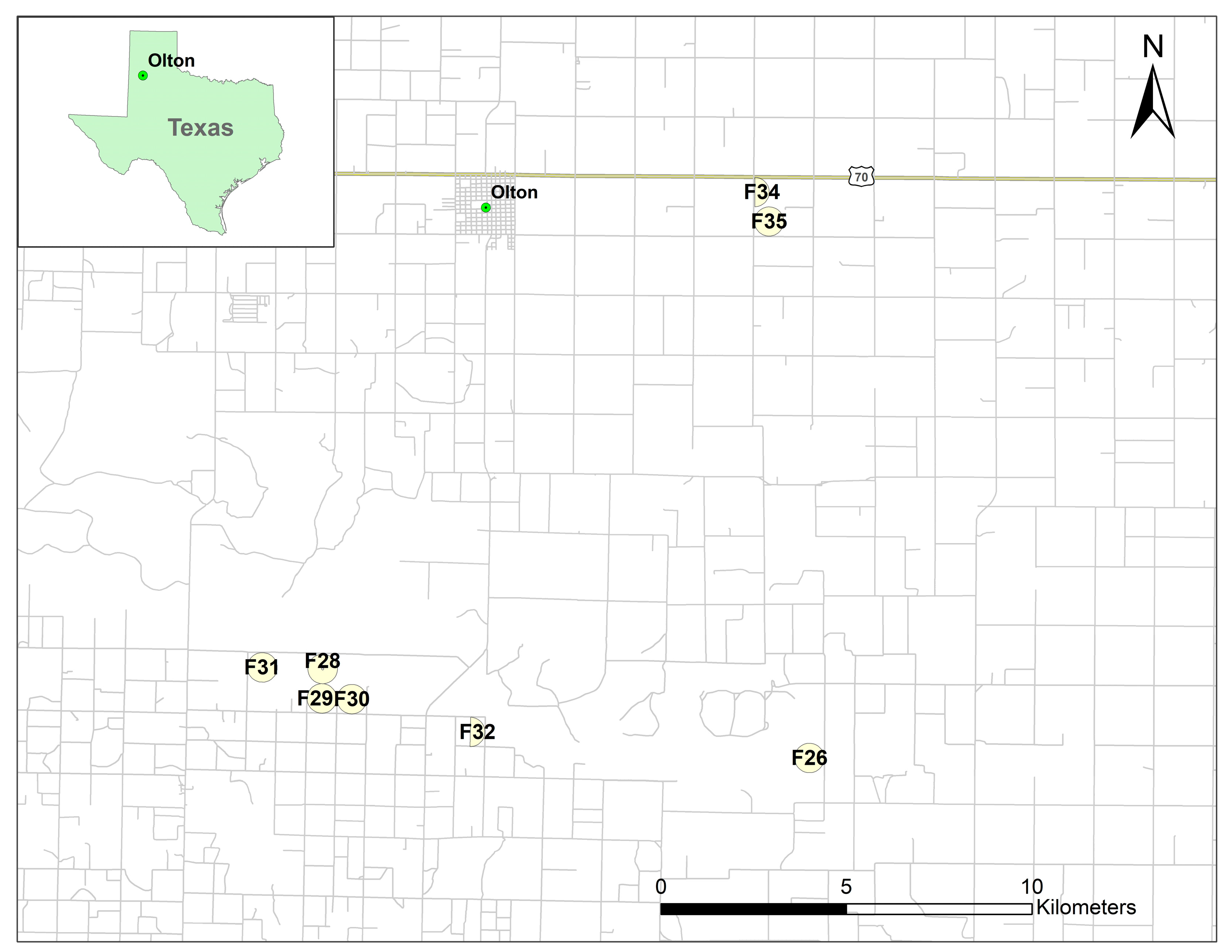
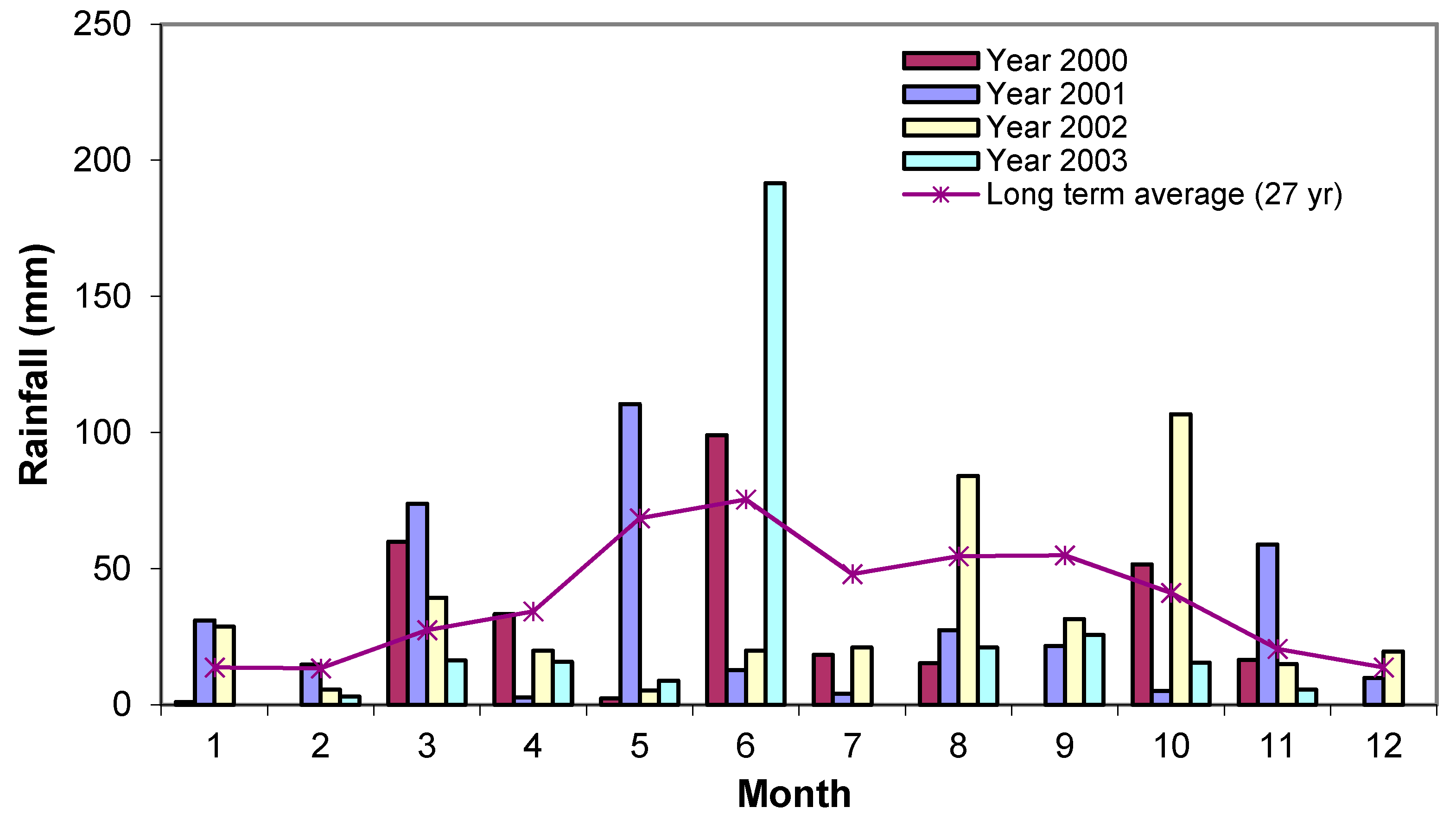
This study was conducted in Lamb County and Hale County in the SHP of Texas (Figure 1). This region has a semiarid climate with an average rainfall ranging from 260 to 600 mm. Irrigation is needed for reliable production in this region [32]. Eight commercially managed fields planted to cotton (Gossypium hirsutum L.) from 2000 to 2003 were selected for this study. The areas of the fields were 50 ha for five full circles (F26, F28, F30, F31, F35), 48 ha for F29, and 25 ha for F32 and F34. However, F34 and F35 were not planted to cotton in 2003. Commercial varieties were used in the fields in these four seasons. Cotton was deficit-irrigated using center pivot irrigation systems. The amount of irrigation varied over the seasons, depending on the precipitation received during the growing season. Approximately 65 kg ha−1 of nitrogen was applied in each field during each growing season. Conservation tillage was practiced in these fields. Planting and harvest dates varied, but were typically in the middle of May and late October, respectively. Monthly precipitation from 2000 to 2003 and long-term average (27 years) was obtained from a weather station approximately 10 km east of F34. The precipitation data is presented in Figure 2.
2.2. Soil Type
Digital soil map units for each field (Figure 3) were obtained from the USDA-NRCS Geospatial Data Gateway (https://datagateway.nrcs.usda.gov). The description of these map units was obtained from the Lamb County soil survey [33] and the Hale County soil survey [34]. On the soil survey map, the units used to delineate the different soils are called map units and can consist of one or more soil series, but mostly just one. Soil map units may contain the same soil series with different slopes and or erosion classes. As shown in Figure 3, a variety of soil types, including sandy, loamy, and clayey soils existed in these study fields. Of all these fields, F29 and F34 were the most homogeneous in terms of soil type with one soil map unit in each field. Most of the soil series in these eight fields belong to the Mollisols or Alfisols orders.
2.3. Data Collection and Preparation
Four years of lint yield data were obtained for six fields (F26, F28, F29, F30, F31, F32), and three years of yield data were obtained for F34 and F35 (2000–2002). Seed cotton yield was collected using a stripper equipped with an optical yield monitor (Model AG700, AGRIplan, Stow, MA, USA) and a differential global positioning system (DGPS) with sub-meter accuracy. Seed cotton yield data was converted to lint yield after ginning the seed cotton. The proportion of lint to seed cotton was typically around 30%. The swath for the harvesting area was 8 m (eight rows) and logging intervals were 1 or 2 s, resulting in a yield data point every 1 or 2 m. Yield data points were subjected to post-harvest screening because yield monitor data normally contains incorrect data points that prevent appropriate interpretation. Removing erroneous data can improve the ability to relate the yield data to other data layers [35]. Yield readings at low speed (<1.6 km h−1) were removed because the harvesting stripper stopped frequently for unloading cotton and other operation related reasons. The remaining data were further screened for yield that exceeds ±3 standard deviations. These yield data cleaning criteria are considered appropriate and have been adopted by many studies [35,36].
Soil apparent electrical conductivity data was collected in each field in the middle of February 2001 using a Veris Model 3100 EC Mapping System (Veris Technologies, Salina, KS, USA) equipped with a differential global positioning system receiver. This system consists of a Wenner array and records ECa in mS m−1 by electrical resistivity at a shallow depth (ECa_sh, 0–30 cm) and a deep depth (ECa_dp, 0–90 cm) simultaneously. Data were collected on transects spaced approximately 15 m apart on a 1 s interval, resulting in a measurement every 3 to 5 m along the transects. This procedure resulted in a data density of 200 to 300 points per ha. The yield data and ECa points in two layers were interpolated into a 30-m raster grid using the Interpolation to Raster routine (inverse distance weighting with the power of two) of the Spatial Analyst in ArcMap (ESRI, Redlands, CA, USA). Cross validation using the spm package in the R software [37] indicated the prediction accuracy was acceptable. For example, the normalized root mean square error (NRMSE) for ECa_dp, calculated as the ration of root mean square error (RMSE) to the mean, ranged from 7.0% for F34 to 13.1% for F28.
2.4. Data Analysis
Temporal yield variability at each landscape position represented by the 30 m grid was evaluated using the equation proposed by Blackmore et al. [6]. The equation for temporal variability is
where is the temporal variance at point i. It shows the deviation from the mean yield over time at point i. is referred to as the temporal standard deviation. t is the time from 2000 to 2003 (2000 to 2002 for fields F34 and F35). Yt,i is yield for year t at point i; and is temporal mean yield for the whole field for years t. n is total number of years involved in the analysis. An area in a field with a low temporal variance value is considered temporally stable across different growing seasons. Conversely, when an area has high temporal variance, the yield is temporally unstable.
To compare the area affected by different levels of temporal variability among different fields [6], a series of temporal standard deviations with an interval of 50 kg ha−1 (0–50 kg ha−1, 50–100 kg ha−1, and so on) and their corresponding percentages of the total field area were summarized. The cumulative percentage of the area of the field affected by different levels of temporal standard deviation was also presented. In this way, one can determine which fields were more sensitive to temporal instability.
Each field was classified into four categories in terms of lint yield and its temporal variance according to Blackmore et al. [6]: (1) high yield area, greater than overall mean yield for all seasons for the field; (2) low yield area, less than the overall mean for all seasons for the field; (3) stable area, low inter-season spatial variance (threshold arbitrarily defined); and (4) unstable area, high inter-season spatial variance (threshold arbitrarily defined). These four classes can have the following combinations: high and stable (HS) representing high yielding with low temporal variance; high and unstable (HU) representing high yielding with high temporal variance; low and unstable (LU) representing low yielding with high temporal variance; and low and stable (LS) representing low yielding with low temporal variance. Analysis of variance (ANOVA) was conducted using the R ANOVA function for each field for the spatial and temporal variability groups in relation to ECa. Mean separation for ECa between these four groups was conducted using the R multcomp package.
3. Results
3.1. Yield Spatial Variability by Season
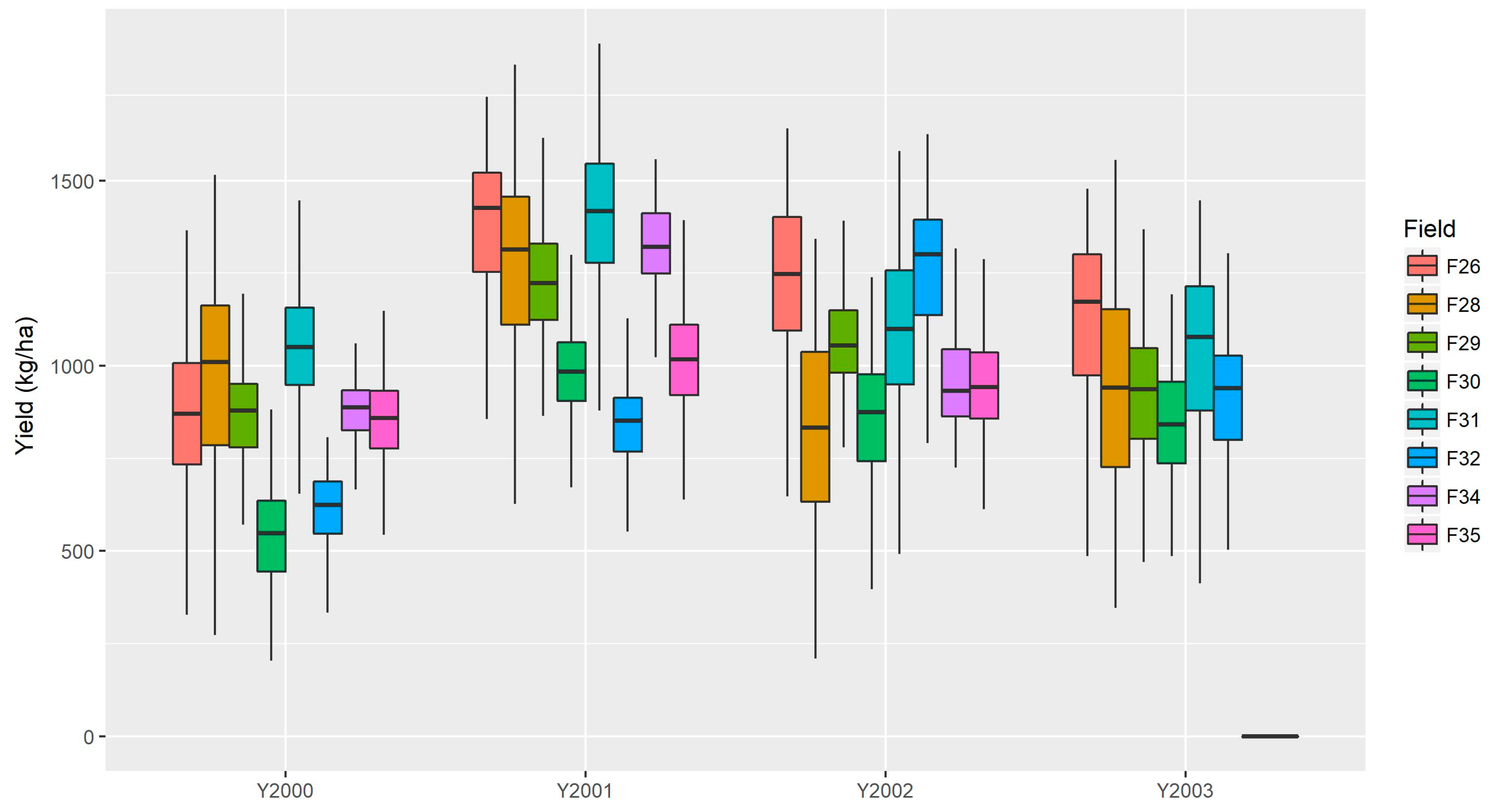
Cotton lint yield had considerable spatial variability in all the eight fields in all the growing seasons (Figure 4). The amount and spatial patterns of variability, however, differed for different fields and seasons. F28 had the greatest spatial variability in yield in the four seasons. The ranges between the minimum and maximum yields were greater than 1100 kg/ha, and coefficients of variation (CVs) were greater than 20% in all the four years. Fields F29 and F34 exhibited the lowest yield variability in all the years. The spatial variability of cotton yield in the other fields was intermediate. Highest yield with the lowest spatial variability occurred in 2001 for all the fields, except for F32. This was probably due to the more favorable weather conditions in that year. Among these four years, 2001 had the highest preseason rainfall, considerably higher than the long-term average rainfall (Figure 2). The greater amount of pre-season rainfall (especially in early May) probably provided more favorable soil water conditions, resulting in a more uniform seedling stand and final yield [14]. Except for F28 and F31, cotton yield in 2000 was the lowest among the four years. This was probably due to the strong insect pressure in the second half growing season in 2000 [12].
3.2. Spatial and Temporal Yield Variability
The relationship between temporal standard deviation and the temporal mean of the yield for each field is presented in Figure 5. Each point on the graph represents a temporal standard deviation and its corresponding temporal mean yield of the growing seasons. These points are divided into four categories using two orthogonal lines representing two thresholds of temporal standard deviation (horizontal line) and temporal mean of the yield (vertical line). As shown in Figure 5, points in the first quadrant (top right section) represent high yield and unstable (HU, high yield with high temporal variation), points in the second quadrant (top left section) represent low yield and unstable (LU), points in the third quadrant (lower left section) represent low yield and stable (LS), and points in the fourth quadrant (lower right section) represent high yield and stable (HS). F29 and F34 had the lowest spatial and temporal variations, demonstrated by more concentrated distribution of points in the spatial and temporal directions (Figure 5). F26, F28, and F31 had the highest spatial and temporal variations, demonstrated by the wide spreads in the spatial and temporal directions. F35 had the highest temporal stability with 90% field area in the temporal stable category (less than 200 kg ha−1 temporal standard deviation).
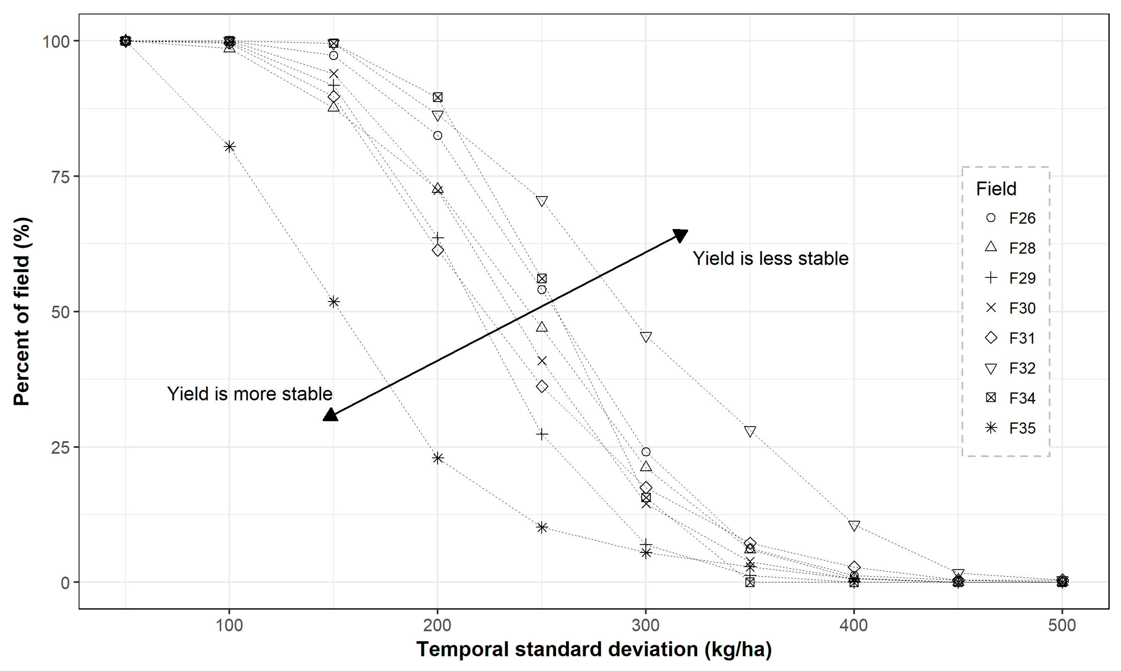
3.3. Temporal Stability
Figure 6 displays the histogram of 10 intervals of temporal standard deviations of yield between 0 and 500 kg ha−1 for each field. The columns represent the area of the field in each interval (left axis) and the lines show the cumulative percentage of the field considered temporally stable at that level (right axis). The sensitivity of temporal stability between a level of temporal standard deviation and the area it affects in the eight fields are shown in Figure 7. The curves are reversed from the cumulative percentage lines in Figure 6 because those curves show the cumulative area of the field affected by increasing temporal variation levels or temporal instability. As shown in these two figures, F35 had the highest temporal stability indicated by more percent area affected by low temporal variations, while F32 had the lowest stability indicated by more percent area affected by high temporal variations. The other fields were intermediate in temporal stability.
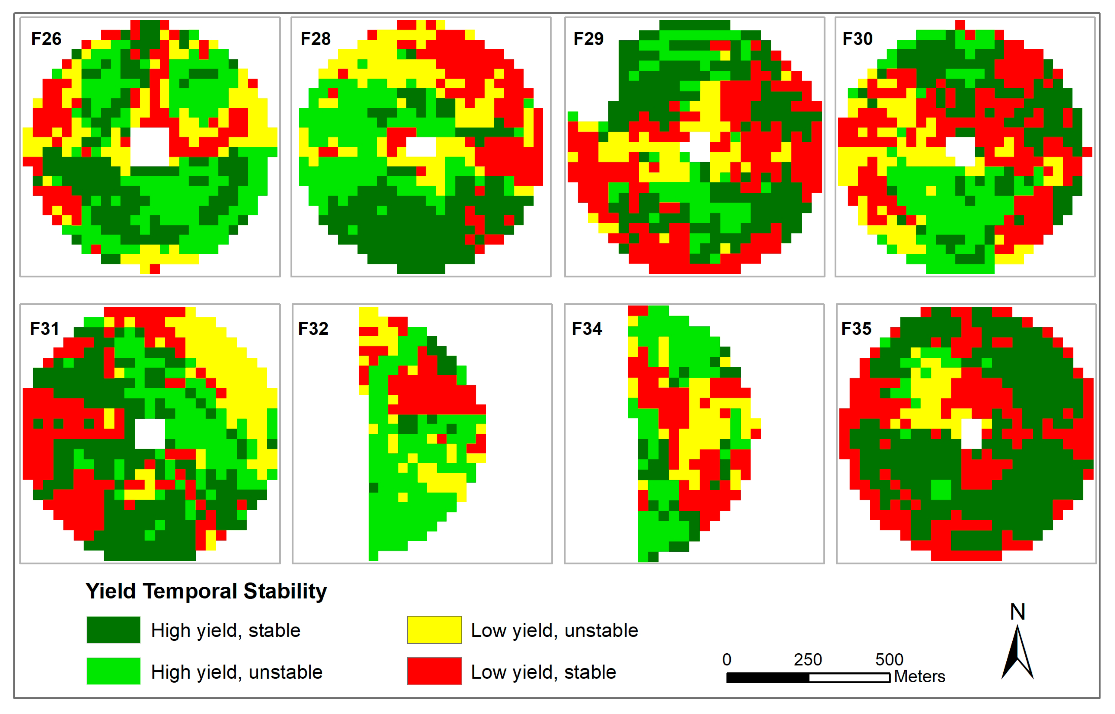
3.4. Spatial and Temporal Trend Maps
Figure 8 shows the spatial and temporal trend map for each field. As described in Section 2.4, each cell (30 m by 30 m) on the map was classified as spatial variability of yield as high or low relative to the overall mean of the specific field; the temporal standard deviation of yield was classified as stable and unstable over time relative to a threshold of 200 kg ha−1. These four basic classes were combined into the following classes: high yield stable (HS), high yield unstable (HU), low yield stable (LS), and low yield unstable (LU). The percentage of each of these four classes for each field are summarized in Table 1. With the exception of southern portions of F28 and F31, yield at the edges of the fields was either consistently low or had a high degree of temporal instability. Previous studies reported similar effect and have attributed this to the operation characteristics of center pivot irrigation systems that cause more run-off water erosion towards the edge of the irrigation system due to higher kinetic energy [6,7]. Consistent with the temporal stability analysis, F35 had the highest yield stability, with approximately 90% of the field area classified as temporally stable (56.1% HS and 33.7% LS); F32 had the lowest yield stability, with 70.6% of the field area classified as unstable (53.2% HU and 17.4% LU).
3.5. Relationship Between ECa and Spatial and Temporal Yield Variability
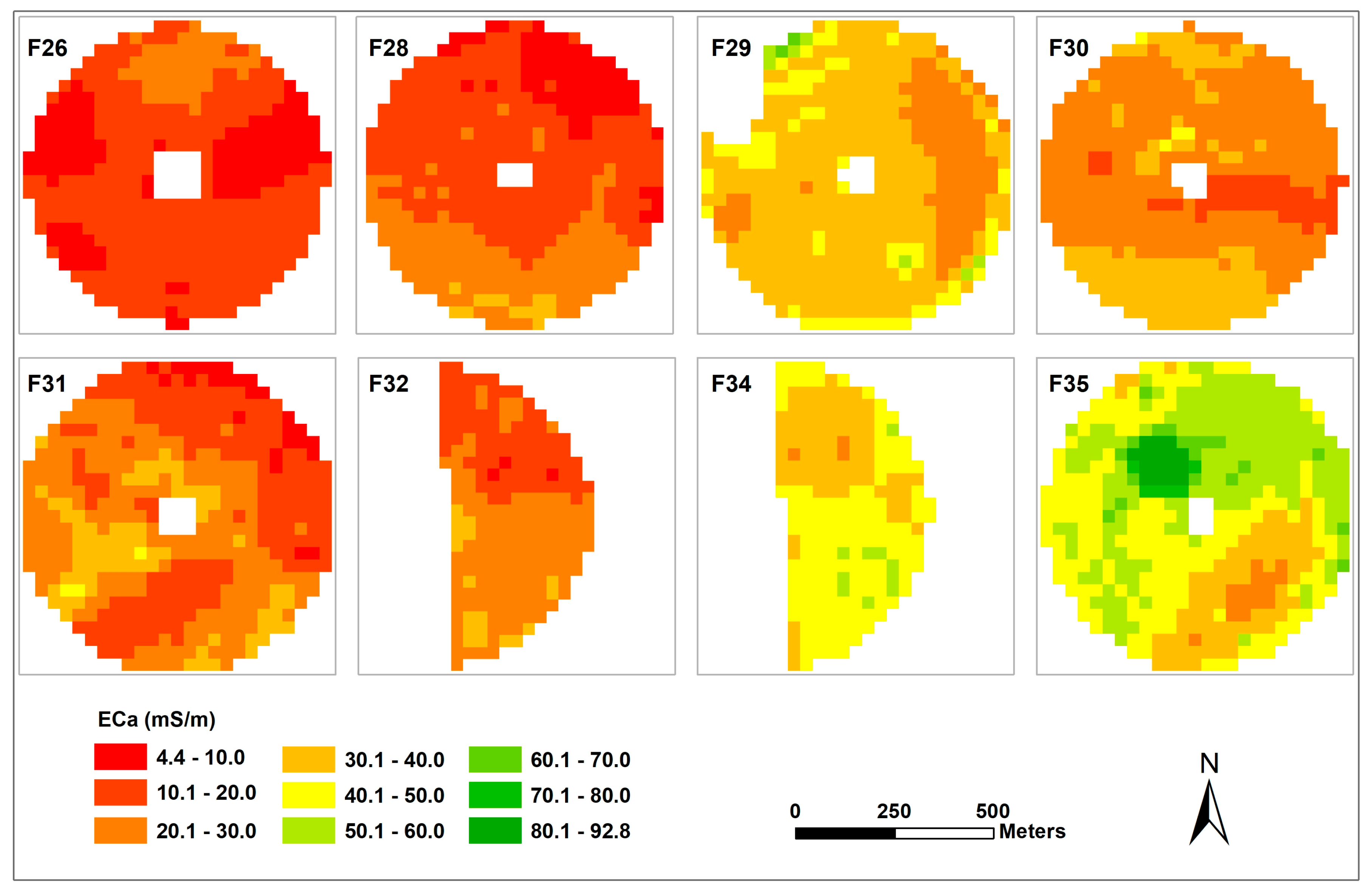
Spatial distribution of ECa (90 cm) for these eight fields is presented in Figure 9. F28 had the greatest variation in ECa (CV = 38.9%) followed by F26 (CV = 35.5) and F31 (CV = 34.2%). F29 and F34 had the lowest spatial variation in ECa, with CVs of 16.2% and 13.3%, respectively. The other fields were intermediate in ECa variation. This is consistent with the soil series distribution: F29 and F34 have one soil map unit in each field.
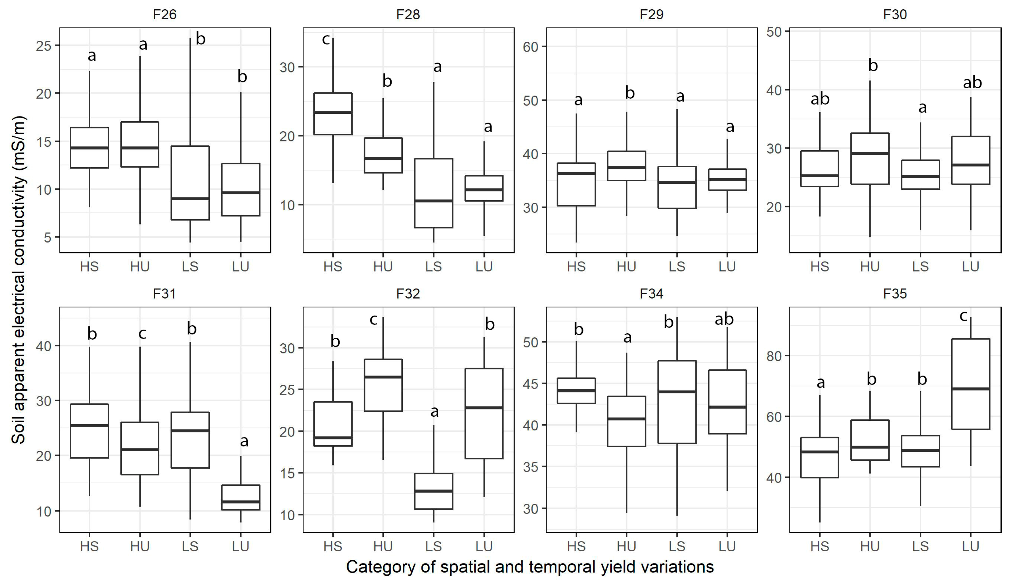
The relationship between spatial and temporal yield variation and ECa varied with the field (Figure 8, Figure 9 and Figure 10). The analysis of variance showed ECa was significantly different (p < 0.05) among different spatial and temporal variation pattern groups for all the fields. For F28 and F26, low yields were mainly distributed in areas with low ECa values. Low and stable yields (LS) were in areas with the lowest ECa values. In these two fields, soils with low ECa in the low yielding areas were mostly sandy soils, such as Brownfield fine sand, Tivoli sand, and Springer loamy fine sand. These soil series are low in productivity because of their high susceptibility to wind erosion and low capacity to hold water and plant nutrients [33]. On average, high and stable yields (HS) were in areas with highest ECa values, where soils are more of loamy series, such as Amarillo series and Spur loam. These soils are more productive because they respond well to the application of nitrogen and phosphate under irrigation [33]. Low and unstable yields (LU) in F31 were located in lowest ECa; low and stable yields (LS) in F32 were located in areas with lowest ECa. For F29, F30, and F34, there was not an obvious relationship pattern between yield spatial and temporal variation and ECa. F35 was a special case. Low and unstable (LU) yield was mainly located in a depression area with high ECa. This area mainly contains a Vertisol consisting of deep and poorly drained clay. These soils swell when wet and shrink when dry, making it challenging for normal farming [33].
4. Discussion
This study showed inter-year variability had a substantial impact on cotton lint yield. The spatial and temporal yield variability patterns varied with the field, soil properties, and weather conditions. Spatial and temporal yield variability, especially for fields with high spatial variability, appeared to be associated with soil ECa. Because ECa is closely related to soil physical properties, such as organic matter, clay content, and cation exchange capacity [17], these properties have a considerable effect on water and nutrient holding capacities, which are major factors influencing crop yield [38]. Water is the first limiting factor for production in the SHP. Therefore, site-specific management of water and nutrient can be based on ECa in fields with a strong association between spatial and temporal variability patterns and ECa (F26, F28, and F35). The inconsistent association between spatial and temporal yield patterns and ECa in other fields indicates some other factors, such as topography and soil chemical properties may play an important role in determining the variability of soil water and nutrient in the field. Weather factors may play a more important role in affecting yield variability in these fields. Further study needs to investigate other factors that influence yield variability in these fields. In addition, F34 and F35 had three years of yield data in this study. Further research with more years of cotton yield data for these two fields is needed to evaluate the consistency in yield temporal trend.
The spatial and temporal variability patterns provide useful information for site-specific management of crop inputs. Management strategies, however, may vary with the field. Fields with high spatial variability and a clear temporal stability pattern, such as F35, F26, and F28, have great potential for long-term site-specific management of crop inputs, such as nitrogen or other fertilizers, irrigation, and other inputs. This study showed crop yields were consistently high or low in specific parts of the field given the same amount of irrigation and crop inputs. This indicates consistently low producing area may not respond well to water and fertilizers. In these areas, the producer may consider reducing irrigation water and other inputs. In the meantime, limited resources may be concentrated on consistently high producing areas (HS), where crops respond well to inputs. These site-specific management practices can increase water and nutrient use efficiencies, as well as reducing environmental risks, such as ground water contamination. The specific amount of input in different areas, however, requires further research. For fields (such as F32) or areas within fields with unstable temporal patterns, long-term site-specific management would be challenging. In these cases, a more appropriate option would be within season site-specific management of crop inputs, such as irrigation, plant growth regulators based on variability in crop growth conditions. Similarly, Blackmore et al. [6] and Silva [7] recommended each growing crop should be managed according to its current needs when yield map trends are not stable.
In this study, high and low yields relative to mean yield of individual fields were used to evaluate spatial patterns of yield distribution. In addition, an arbitrary temporal variance was selected across different fields. For site-specific management, more yield classes, such as high, medium, and low in combination with a separate threshold of temporal yield variance might provide management at finer scales. Ideally, incorporating profitability evaluation in such spatial and temporal yield analysis provides a more realistic site-specific management strategy. Thus, a spatial and temporal profitability analysis should be considered for future studies.
5. Conclusions
Cotton yield had substantial spatial and temporal variability. The amount and pattern of spatial and temporal variation varied with fields. For fields with high variability, spatial and temporal yield patterns are related to ECa, indicating that soil properties related to ECa, such as soil texture and water holding capacity in this region, are the major factors influencing yield variability in these fields. For fields with low variability, spatial and temporal yield patterns might be more influenced by weather or other factors in different growing seasons. Because each field is unique in spatial and temporal yield patterns, the site-specific management strategy should be different for different fields. Fields with high spatial variability and a clear temporal stability pattern have great potential for long-term site-specific management of crop inputs. The application of ECa for site-specific management is limited to fields with high spatial variability and with a strong association between yield spatial patterns and ECa variation patterns. For example, the farm manager may consider reducing crop inputs, such as nitrogen or other fertilizers and irrigation in consistently low yielding areas and concentrate crop inputs in high yielding areas to optimize production and profitability. For unstable yield, however, long-term management practices are difficult to implement. For these fields, within season site-specific management can be a better choice. Variable rate application of water, plant growth regulators, nitrogen, harvest aids, etc. may be implemented based on the spatial variability of crop growth conditions at specific times. Future research needs to evaluate other factors such as topography, soil physical and chemical properties that affect yield variability. Further research needs also to assess spatial and temporal variability in profitability within the field for more practical decision support of site-specific management.
Funding
This work was support by a grant from Cotton Incorporated.
Acknowledgments
The author would like to thank Brightbill Farms for providing the yield and soil EC data in this research.
Conflicts of Interest
The author declares no conflict of interest.
References
- Miller, M.P.; Singer, M.J.; Nielsen, D.R. Spatial variability of wheat yield and soil properties on complex hills. Soil Sci. Soc. Am. J. 1988, 52, 1133–1141. [Google Scholar] [CrossRef]
- Pierce, F.J.; Nowak, P. Aspects of precision agriculture. Adv. Agron. 1999, 67, 1–85. [Google Scholar]
- Dobermann, A.; Ping, J.L.; Adamchuk, V.I.; Simbahan, G.C.; Ferguson, R.B. Classification of crop yield variability in irrigated production fields. Agron. J. 2003, 5, 1105–1120. [Google Scholar] [CrossRef]
- Wibawa, W.D.; Dludlu, D.L.; Swenson, L.J.; Hopkins, D.G.; Dahnke, W.C. Variable fertilizer application based on yield goal, soil fertility, and soil map unit. JPA 1993, 6, 255–261. [Google Scholar] [CrossRef]
- Machado, S.; Bynum, E.D.; Archer, T.L.; Bordovsky, J.; Rosenow, D.T.; Peterson, C.; Bronson, K.; Nesmith, D.M.; Lascano, R.J.; Wilson, L.T.; et al. Spatial and temporal variability of sorghum grain yield: Influence of soil, water, pests, and diseases relationships. Precis. Agric. 2002, 3, 389–406. [Google Scholar] [CrossRef]
- Blackmore, S.; Godwin, R.J.; Fountas, S. The analysis of spatial and temporal trends in yield map data over six years. Biosyst. Eng. 2003, 84, 455–466. [Google Scholar] [CrossRef]
- Marques da Silva, J.R. Analysis of the spatial and temporal variability of irrigated maize yield. Biosyst. Eng. 2006, 94, 337–349. [Google Scholar] [CrossRef]
- Johnson, R.M.; Downer, R.G.; Bradow, J.M.; Bauer, P.J.; Sadler, E.J. Variability in cotton fiber yield, fiber quality, and soil properties in a Southeastern Coastal Plain. Agron. J. 2002, 94, 1305–1316. [Google Scholar] [CrossRef]
- Yang, C.; Everitt, J.H.; Bradford, J.M.; Murden, D. Airborne Hyperspectral imagery and yield monitor data for mapping cotton yield variability. Precis. Agric. 2004, 5, 445–461. [Google Scholar] [CrossRef]
- Corwin, D.L.; Lesch, S.M.; Shouse, P.J.; Soppe, R.; Ayars, J.E. Identifying soil properties that influence cotton yield using soil sampling directed by apparent soil electrical conductivity. Agron. J. 2003, 95, 352–364. [Google Scholar] [CrossRef]
- Ping, J.L.; Green, C.J.; Bronson, K.F.; Zartman, R.E.; Dobermann, A. Identification of relationships between cotton yield, quality, and soil properties. Agron. J. 2004, 96, 1588–1597. [Google Scholar] [CrossRef]
- Bronson, K.F.; Wayne Keeling, J.; Booker, J.D.; Chua, T.T.; Wheeler, T.A.; Boman, R.K.; Lascano, R.J. Influence of landscape position, soil series, and phosphorus fertilizer on cotton lint yield. Agron. J. 2003, 95, 949–957. [Google Scholar] [CrossRef]
- Elms, M.K.; Green, C.J.; Johnson, P.N. Variability of cotton yield and quality. Commun. Soil Sci. Plant Anal. 2001, 32, 351–368. [Google Scholar] [CrossRef]
- Guo, W.; Maas, S.J.; Bronson, K.F. Relationship between cotton yield and soil electrical conductivity, topography, and Landsat imagery. Precis. Agric. 2012, 13, 678–692. [Google Scholar] [CrossRef]
- Swinton, S.M.; Lowenberg-DeBoer, J. Evaluating the profitability of site-specific farming. JPA 1998, 11, 439–446. [Google Scholar] [CrossRef]
- Kravchenko, A.N.; Bullock, D.G. Correlation of corn and soybean grain yield with topography and soil properties. Agron. J. 2000, 92, 75–83. [Google Scholar] [CrossRef]
- Corwin, D.L.; Lesch, S.M. Application of soil electrical conductivity to precision agriculture. Agron. J. 2003, 95, 455–471. [Google Scholar] [CrossRef]
- Corwin, D.L.; Lesch, S.M. Apparent soil electrical conductivity measurements in agriculture. Comput. Electron. Agric. 2005, 46, 11–43. [Google Scholar] [CrossRef]
- Kravchenko, A.N.; Thelen, K.D.; Bullock, D.G.; Miller, N.R. Relationship among crop grain yield, topography, and soil electrical conductivity studied with cross-correlograms. Agron. J. 2003, 95, 1132–1139. [Google Scholar] [CrossRef]
- Bronson, K.F.; Onken, A.B.; Booker, J.D.; Lascano, R.J.; Provin, T.L.; Torbert, H.A. Irrigated cotton lint yields as affected by phosphorus fertilizer and landscape position. Commun. Soil Sci. Plant Anal. 2001, 32, 1959–1967. [Google Scholar] [CrossRef]
- Lund, E.D.; Christy, C.D.; Drummond, P.E. Using yield and soil electrical conductivity (EC) maps to derive crop production performance information. In Proceedings of the 5th International Conference on Precision Agriculture, Bloomington, MN, USA, 16–19 July 2000. [Google Scholar]
- Clay, D.E.; Chang, J.; Malo, D.D.; Carlson, C.G.; Reese, C.; Clay, S.A.; Ellsbury, M.; Berg, B. Factors influencing spatial variability of soil apparent electrical conductivity. Commun. Soil Sci. Plant Anal. 2001, 32, 2993–3008. [Google Scholar] [CrossRef]
- Medeiros, W.N.; de Queiroz, D.M.; Valente, D.S.; de Carvalho Pinto, F.D.; Melo, C.A. The temporal stability of the variability in apparent soil electrical conductivity. Biosci. J. 2016, 32, 150–159. [Google Scholar] [CrossRef] [Green Version]
- Singh, G.; Williard, K.; Schoonover, J. Spatial relation of apparent soil electrical conductivity with crop yields and soil properties at different topographic positions in a small Agricultural Watershed. Agronomy 2016, 6, 57. [Google Scholar] [CrossRef]
- Kitchen, N.R.; Drummond, S.T.; Lund, E.D.; Sudduth, K.A.; Buchleiter, G.W. Soil electrical conductivity and topography related to yield for three contrasting soil-crop systems. Agron. J. 2003, 95, 483–495. [Google Scholar] [CrossRef]
- Humphreys, M.T.; Raun, W.R.; Martin, K.L.; Freeman, K.W.; Johnson, G.V.; Stone, M.L. Indirect estimates of soil electrical conductivity for improved prediction of wheat grain yield. Commun. Soil Sci. Plant Anal. 2005, 35, 2639–2653. [Google Scholar] [CrossRef]
- Stadler, A.; Rudolph, S.; Kupisch, M.; Langensiepen, M.; van der Kruk, J.; Ewert, F. Quantifying the effects of soil variability on crop growth using apparent soil electrical conductivity measurements. Eur. J. Agron. 2015, 64, 8–20. [Google Scholar] [CrossRef]
- Gholizadeh, A.; Amin Mohd Soom, M.; Anuar, A.R.; Aimrun, W. Relationship between apparent electrical conductivity and soil physical properties in a Malaysian paddy field. Arch. Agron. Soil Sci. 2012, 58, 155–168. [Google Scholar] [CrossRef]
- Ezrin, M.H.; Amin, M.S.M.; Anuar, A.R.; Aimrun, W. Relationship between rice yield and apparent electrical conductivity of paddy soils. Am. J. Appl. Sci. 2010, 7, 63–70. [Google Scholar] [CrossRef]
- Chan, C.S.; Amin, M.S.; Lee, T.S.; Mohammud, C.H. Apparent soil electrical conductivity as an indicator of paddy soil productivity. J. Trop. Agric. Food Sci. 2008, 36, 145–153. [Google Scholar]
- McBratney, A.; Whelan, B.; Ancev, T.; Bouma, J. Future directions of precision agriculture. Precis. Agric. 2005, 6, 7–23. [Google Scholar] [CrossRef]
- Mauget, S.A.; Adhikari, P.; Leiker, G.; Baumhardt, R.L.; Thorp, K.R.; Ale, S. Modeling the effects of management and elevation on West Texas dryland cotton production. Agric. For. Meteorol. 2017, 247, 385–398. [Google Scholar] [CrossRef]
- USDA Soil Conservation Service. Soil Survey of Lamb County, Texas; Newman, A.L., Ed.; United States Department of Agriculture, Soil Conservation Service: Washington, DC, USA, 1962.
- USDA Soil Conservation Service. Soil Survey of Hale County, Texas; Blakely, E.R., Koos, W.M., Eds.; USDA: Washington, DC, USA, 1974.
- Kleinjan, J.; Chang, J.; Wilson, J.; Humburg, D.; Carlson, G.; Clay, D.; Long, D. Cleaning Yield Data; SDSU Publication: San Diego, CA, USA, 2002. [Google Scholar]
- Simbahan, G.C.; Dobermann, A.; Ping, J.L. Site specific management: Screening yield monitor data improves grain yield maps. Agron. J. 2004, 96, 1091–1102. [Google Scholar] [CrossRef]
- R Core Team. R: A Language and Environment for Statistical Computing; The R Foundation for Statistical Computing: Vienna, Austria, 2018. [Google Scholar]
- Jaynes, D.B.; Colvin, T.S.; Ambuel, J. Yield mapping by electromagnetic induction. In Proceedings of the Site Specific Management for Agricultural Systems, Minneapolis, MN, USA, 27–30 March 1994; pp. 383–393. [Google Scholar]
Figure 1.
Locations of eight commercially managed irrigated fields for the study in the Southern High Plains.
Figure 1.
Locations of eight commercially managed irrigated fields for the study in the Southern High Plains.

Figure 2.
Monthly precipitation of 2000 to 2003 and long-term precipitation at Halfway, Texas.

Figure 3.
Soil map units in eight fields in the Southern High Plains. AfA: Amarillo fine sandy loam, 0–1% slopes (Fine-loamy, mixed, superactive, thermic Aridic Paleustalfs); AfB: Amarillo fine sandy loam, 1–3% slopes (Fine-loamy, mixed, superactive, thermic Aridic Paleustalfs); AIA: Amarillo loam, 0–1% slopes (Fine-loamy, mixed, superactive, thermic Aridic Paleustalfs); AIB: Amarillo loam, 1–3% slopes (Fine-loamy, mixed, superactive, thermic Aridic Paleustalfs); AmB: Amarillo loamy fine sand, 0–3% slopes (Fine-loamy, mixed, superactive, thermic Aridic Paleustalfs); Br: Brownfield fine sand (Loamy, mixed, superactive, thermic Arenic Aridic Paleustalfs); EsB: Estacado loam, 1–3% slopes (Fine-loamy, mixed, superactive, thermic Aridic Paleustolls); MfA: Mansker fine sandy loam, 0–1% slopes (Fine-loamy, carbonatic, thermic Calcidic Paleustolls); MfB: Mansker fine sandy loam, 1–3 % slopes (Fine-loamy, carbonatic, thermic Calcidic Paleustolls); MkA: Mansker loam, 0–1% slopes (Fine-loamy, carbonatic, thermic Calcidic Paleustolls); OtA: Olton loam, 0–1% slope (Fine, mixed, superactive, thermic Aridic Paleustolls); OtB: Olton loam, 1–2% slope (Fine, mixed, superactive, thermic Aridic Paleustolls); PfB: Portales fine sandy loam, 1–3% slopes (Fine-loamy, mixed, superactive, thermic Aridic Calciustolls); PuA: Pullman clay loam, 0–1% slope (Fine, mixed, superactive, thermic Torrertic Paleustolls); Ra: Randall clay (Fine, smectitic, thermic Ustic Epiaquerts); Sf: Springer fine sandy loam, undulating (Coarse-loamy, mixed, superactive, thermic Typic Paleustalfs); Sh: Springer loamy fine sand, hummocky (Coarse-loamy, mixed, superactive, thermic Typic Paleustalfs); SpB: Spur fine sandy loam, 1–3% slopes (Fine-loamy, mixed, superactive, thermic Fluventic Haplustolls); Tv: Tivoli fine sand (Mixed, thermic Typic Ustipsamments); ZmB: Zita loam, 1–2% slopes (Fine-loamy, mixed, superactive, thermic Aridic Haplustolls).

Figure 4.
Cotton lint yield variability of eight fields in the Southern High Plains 2000 to 2003.

Figure 5.
Relationship between temporal standard deviation and temporal mean cotton yield from 2000 to 2003 for eight fields in the Southern High Plains.
Figure 5.
Relationship between temporal standard deviation and temporal mean cotton yield from 2000 to 2003 for eight fields in the Southern High Plains.

Figure 6.
Frequency distribution by area (ha) of temporal standard deviation of cotton yield for eight fields in the Southern High Plains 2000–2003.
Figure 6.
Frequency distribution by area (ha) of temporal standard deviation of cotton yield for eight fields in the Southern High Plains 2000–2003.

Figure 7.
Percentage of field area affected by temporal instability of yield for eight cotton fields in the Southern High Plains 2000–2003.
Figure 7.
Percentage of field area affected by temporal instability of yield for eight cotton fields in the Southern High Plains 2000–2003.

Figure 8.
Spatial and temporal trend maps of cotton yield with 200 kg ha−1 yield temporal stability threshold for eight fields in the Southern High Plains.
Figure 8.
Spatial and temporal trend maps of cotton yield with 200 kg ha−1 yield temporal stability threshold for eight fields in the Southern High Plains.

Figure 9.
Variation of soil apparent electrical conductivity (ECa, 90 cm) in eight fields in the Southern High Plains.
Figure 9.
Variation of soil apparent electrical conductivity (ECa, 90 cm) in eight fields in the Southern High Plains.

Figure 10.
Relationship between spatial temporal yield variations of cotton yield and distribution of soil apparent electrical conductivity (ECa) in eight fields in the Southern High Plains 2000–2003. HS: high yield and stable; HU: high yield and unstable; LS: low yield and stable; LU: low yield and unstable. Letters on top of boxes mark significant differences in ECa between spatial and temporal yield pattern groups. Pairs of groups that are not significantly different from one another share the same letter (p < 0.05).


Table 1.
Spatial and temporal trend area in percentage with a yield stability threshold of 200 kg ha−1.
Table 1.
Spatial and temporal trend area in percentage with a yield stability threshold of 200 kg ha−1.
| Field | HS, % | LS, % | Sum S, % | HU, % | LU, % | Sum U, % |
|---|---|---|---|---|---|---|
| F26 | 27.7 | 18.3 | 46.0 | 34.2 | 19.8 | 54.0 |
| F28 | 30.2 | 22.8 | 53.0 | 25.8 | 21.2 | 47.0 |
| F29 | 36.4 | 36.3 | 72.7 | 14.5 | 12.8 | 27.3 |
| F30 | 25.0 | 34.1 | 59.1 | 23.8 | 17.1 | 40.9 |
| F31 | 37.6 | 26.2 | 63.8 | 19.5 | 16.7 | 36.2 |
| F32 | 6.0 | 23.4 | 29.4 | 53.2 | 17.4 | 70.6 |
| F34 | 12.7 | 31.3 | 44.0 | 34.3 | 21.7 | 56.0 |
| F35 | 56.1 | 33.7 | 89.8 | 3.9 | 6.3 | 10.2 |
HS, high yield and stable; HU, high yield and unstable; LS, low yield and stable; LU, low yield and unstable; Sum S, the sum of area with low inter-annual variance; Sum U, the sum of area with high inter-annual variance.
© 2018 by the author. Licensee MDPI, Basel, Switzerland. This article is an open access article distributed under the terms and conditions of the Creative Commons Attribution (CC BY) license (http://creativecommons.org/licenses/by/4.0/).
Share and Cite
MDPI and ACS Style
Guo, W. Spatial and Temporal Trends of Irrigated Cotton Yield in the Southern High Plains. Agronomy 2018, 8, 298. https://0-doi-org.brum.beds.ac.uk/10.3390/agronomy8120298
AMA Style
Guo W. Spatial and Temporal Trends of Irrigated Cotton Yield in the Southern High Plains. Agronomy. 2018; 8(12):298. https://0-doi-org.brum.beds.ac.uk/10.3390/agronomy8120298
Chicago/Turabian StyleGuo, Wenxuan. 2018. "Spatial and Temporal Trends of Irrigated Cotton Yield in the Southern High Plains" Agronomy 8, no. 12: 298. https://0-doi-org.brum.beds.ac.uk/10.3390/agronomy8120298
Note that from the first issue of 2016, this journal uses article numbers instead of page numbers. See further details here.