Water Stress Permanently Alters Shoot Architecture in Common Bean Plants


1
Agricultural Meteorology Group, Crop Science Department, Federal University of Santa Maria, Av. Roraima, 1000, Santa Maria 97105-900, Brazil
2
Centre for Crop Systems Analysis, Wageningen University and Research Centre, P.O. Box 430, 6700 AK Wageningen, The Netherlands
3
Soil Physics and Land Management Group, Wageningen University and Research Centre, P.O. Box 47, 6700 AA Wageningen, The Netherlands
4
Soil Physics Laboratory, Center for Nuclear Energy in Agriculture, University of São Paulo, P.O. Box 96, Piracicaba 13405-900, Brazil
*
Author to whom correspondence should be addressed.
Agronomy 2019, 9(3), 160; https://0-doi-org.brum.beds.ac.uk/10.3390/agronomy9030160
Submission received: 24 February 2019
/
Revised: 17 March 2019
/
Accepted: 19 March 2019
/
Published: 26 March 2019
(This article belongs to the Special Issue Model Application for Sustainable Agricultural Water)
Abstract
:The effects of water stress on crop yield through modifications of plant architecture are vital to crop performance such as common bean plants. To assess the extent of this effect, an outdoor experiment was conducted in which common bean plants received five treatments: fully irrigated, and irrigation deficits of 30% and 50% applied in flowering or pod formation stages onwards. Evapotranspiration, number and length of pods, shoot biomass, grain yield and harvest index were assessed, and architectural traits (length and thickness of internodes, length of petioles and petiolules, length and width of leaflet blades and angles) were recorded and analyzed using regression models. The highest irrigation deficit in the flowering stage had the most pronounced effect on plant architecture. Stressed plants were shorter, leaves were smaller and pointing downward, indicating that plants permanently altered their exposure to sunlight. The combined effect of irrigation deficit and less exposure to light lead to shorter pods, less shoot biomass and lower grain yield. Fitted empirical models between water deficit and plant architecture can be included in architectural simulation models to quantify plant light interception under water stress, which, in turn, can supply crop models adding a second order of water stress effects on crop yield simulation.
1. Introduction
Water stress is one of the main abiotic stresses limiting crop production in many tropical and subtropical regions [1,2] determining rainfed agricultural production [3,4,5]. There are indications that the risk of drought may yet increase with the expected climate change in drought-prone areas [6]. An increase in the intensity, duration and area affected by drought has been observed in tropical and subtropical areas since the 1970s [7]. In these regions, an increase in air temperature and decrease in precipitation have contributed to enhanced dry conditions placing additional pressure on agricultural systems [8,9].
During a crop growth cycle, water is needed for photosynthesis, maintenance of turgor and cooling of leaves. When water supply becomes inadequate, stomata will close, affecting CO2 assimilation and transpiration [10]. Water shortage reduces the availability of CO2 in the leaf tissues, and thus the production of assimilates and growth, introducing limitations to the productivity mainly on C3 plants [11,12].
Plants also adapt their architectural development to the available resources, and differ in plasticity to adapt to abiotic stresses [13]. Sunlight interception by plants depends on plant architecture. It is considered to be described by the Lambert Beer law of exponential extinction as a function of the leaf area index and the angular distribution of leaves [14]. Under water stress, the daily paraheliotropic movement of leaves modify its angular distribution and changes the exponential interception of sunlight inside the canopy [15]. Leaves change their angular distribution from planophile to vertical positions as a result of water stress in soybean (Glycine max L. Merr.) [16]. Using this mechanism, leaves were able to diminish the incidence of direct sunrays and to reduce plant energy load, transpiration and temperature, leading to less sunlight being intercepted and more sunlight reaching the soil surface.
The common bean (Phaseolus vulgaris L.) provides an important source of calories and protein for humans [17,18], and is frequently grown under water-limited conditions. Production regions are located mainly in developing tropical and subtropical areas [19,20], yielding approximately 12 million tons globally and 5.5 and 2.5 million tons in Latin America and Africa, respectively [21,22]. Drought affects 73% of the area planted to beans in Latin America, for example [23,24].
Bean plants are sensitive to water stress, mainly because of their shallow root system [25]. Bean seed quality (hardness) as well as vigor and dry matter yield are negatively affected by water shortage [26,27]. Reduction of grain yield by water stress in bean plants has been reported in several studies [20,28,29]. When water stress occurs during the flowering stage, the reduction tends to be more pronounced [30] due to the high crop water consumption during flowering [31]. Sensitivity to water stress is higher during reproductive phase (flowering and pod formation) than during the vegetative growth phase [32,33].
Many traits in common beans are affected by water stress, including a reduced number of leaves, reduced leaf size and inhibition of the expansion of foliage [34], shedding of leaves, flowers and young fruits [35]. The reduction of leaf area, i.e., the photosynthetic surface, results in a decrease in dry matter accumulation [33]. Water deficit imposed during the reproductive development may decrease the number of flowers, pods and number of seeds per pod [36]. The total number of flowers in some varieties may be reduced significantly under drought reducing the number of pods per plant [37]. Withholding water to plants at floral initiation and at 50% podding stage leads to pod abortion rates of 21 and 65%, respectively [38].
Although several aspects of common bean response to water stress, such as water consumption, leaf area and number of reproductive organs are well documented [29,39,40,41], detailed information and description on shoot architecture and how it interacts with water stress is currently lacking. For example, the size of internodes, petioles and petiolules and angles between plant organs, as well as the numerical description of these architectural traits (including leaves) along the vertical plant axis, have never been quantified.
In order to understand how plant architecture in common bean is affected by water shortage and how these changes in plant architecture affect crop performance, we assessed plant architecture traits of common bean plants at different levels of water shortage during the reproductive phase.
2. Materials and Methods
2.1. Experimental Set-Up
All measurements were made in an experiment with common bean (Phaseolus vulgaris L., cv. Berna) conducted from May to August 2014 in Wageningen, The Netherlands (51°59′20″ N, 5°39′16″ E). On 15 May, bean seeds were sown at 2 to 3 cm depth in a soil substrate [N supply capacity, 55 kg N ha−1 year−1; organic matter, 3.1% with a C/N ratio of 15; soil mineral N content before sowing (0–25 cm), 1240 mg N kg−1] contained in 7 L plastic pots (0.21 m top diameter, 0.16 m bottom diameter, 0.27 m depth). Pots were placed on a table in the open air under a permanent rain sheltering roof of transparent plastic (EVA 200 micron clear film). Placed in a square grid, the distance between pot centers was 0.25 m with a total of 16 plants m−2, a common plant density in bean cropping [42].
Five irrigation treatments were imposed: a fully irrigated control treatment and four deficit irrigation treatments. Each treatment consisted of 20 plants. Five plants per treatment were tagged in the beginning of the crop cycle. Yield components at the end of the crop cycle were determined for all plants and architectural traits were determined for the five tagged plants. It is common to interrupt irrigation completely after reaching a specific development phase when plants are grown in large pots [29] or in the field [43]. However, as we used small 7 L plastic pots to facilitate manipulation of plants during architecture measurements, thus imposing a smaller soil volume to the root systems, irrigation was not completely interrupted but instead continued at lower levels in the four treatments until the end of the crop cycle. This warranted plant survival while still imposing water limitation. Two irrigation deficit intensities relative to the water amount in the control treatment (−30%-Low deficit (L) and −50%-High deficit (H)) were applied during two different stages: at the onset of the flowering (F) stage (43 days after sowing—27 June) in treatments FL and FH, respectively, and at the onset of the pod (P) formation stage (48 days after sowing—2 July) in treatments PL and PH, respectively. The onset of the flowering and pod formation stages was considered when 50% of the plants presented one open flower and one pod at maximum length, respectively.
Five pots randomly chosen from each treatment were weighed three times per week. The amount of water to be applied was calculated by taking into account the weight of pots of the control treatment and comparing them to a reference weight taken at the beginning of the experiment immediately after a full irrigation when a tensiometer reading indicated a pressure head in the order of 2.5 m, comparable to field capacity. A logistic growth curve for common bean plants was used to correct for the fresh weight of plants [44]. Weight measurements were also used to estimate the mean evapotranspiration rate during the crop cycle.
Harvest occurred 105 days after sowing, on 28 August, and yield components were determined. Final number of pods was counted and the final length of pods (m) was measured. All plants were dried for 24 h in an oven at 70 °C before determining shoot biomass (stem + pod + leaves) (g plant−1). Grains were separated from pods and the grain yield (g plant−1) was measured. Harvest index (HI) was then calculated dividing grain yield by shoot biomass.
2.2. Plant Architecture Data
2.2.1. General Bean Plant Architecture
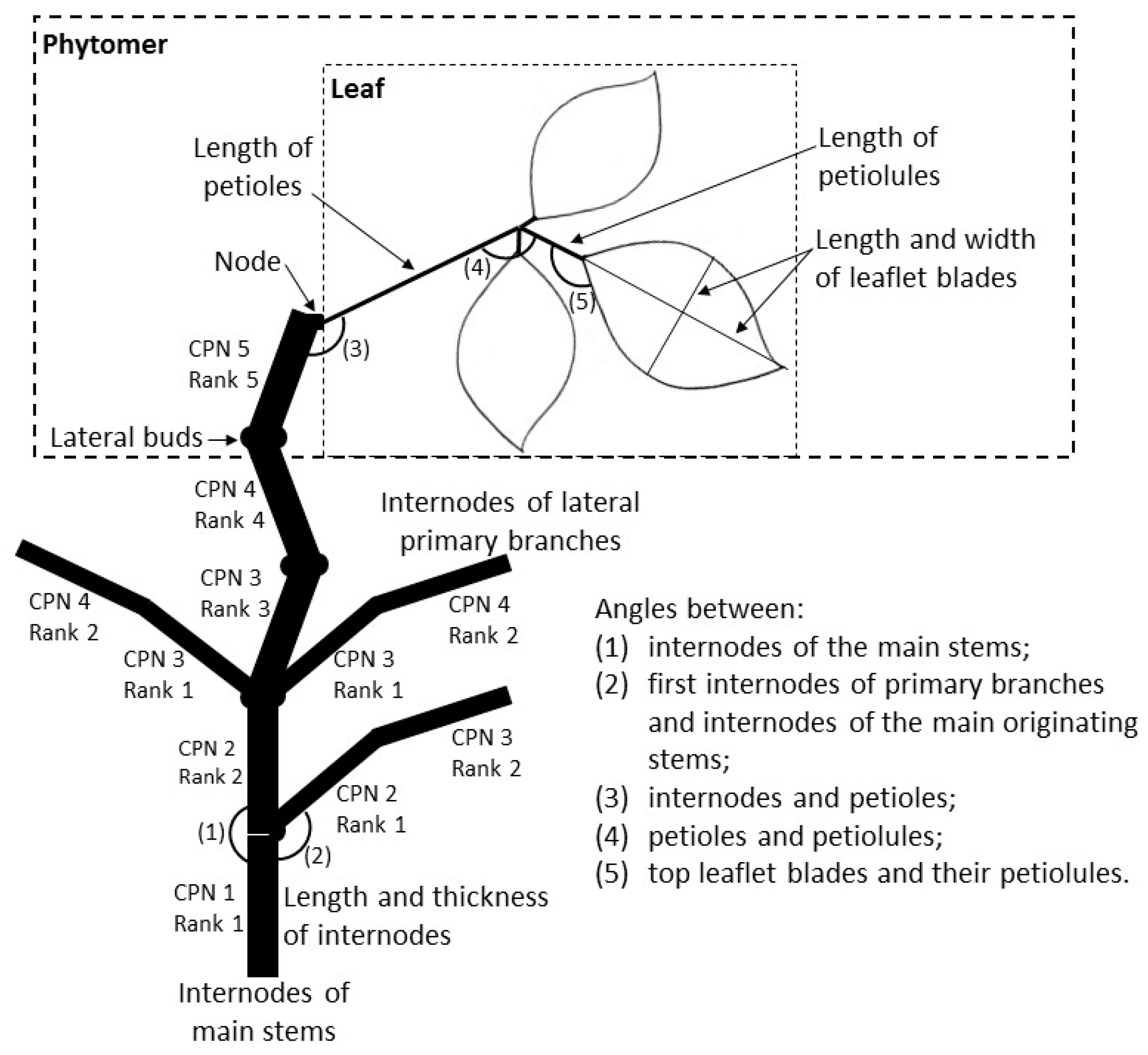
Common bean plants are composed of a main stem and an abundant number of lateral primary branches with leaves and flowers [45]. The unit for an architectural analysis of the bean plant in terms of measurements was the phytomer [46]. A phytomer by definition comprises an internode with a lateral bud at the bottom, a node above the internode, a petiole inserted on the node, and a leaf [47]. Given this starting point, the architecture of the bean plant is defined in Figure 1 in terms of a sequence of numbered phytomers. The first phytomer of the main stem (#1) does not contain leaves but has lateral buds that grow out into branches. The subsequent phytomers—2, 3, 4 and 5—have two lateral buds each, placed on opposite sides. There is only one lateral bud on phytomers above the fifth phytomer of the main stem. From phytomer 3 onwards, the main stem is composed of internodes that follow a sympodial pattern that gives rise to a typical zigzag shape. Leaves are trifoliate, consisting of a petiole, two asymmetrical ovalate side leaflets and one symmetrical top leaflet in the middle with a longer petiolule (top leaflet petiole) than that of lateral ones. The exception is the second phytomer of the main stem, which carries two single leaves with petioles only. Reproductive organs (flower buds, flowers and pods) are organized in racemes. The cultivar used in this study has an indeterminate growth habit, and development of new vegetative structures continues in the reproductive phase.
2.2.2. Air Temperature
Thermal time (°Cd) was calculated with the daily mean air temperature inside the canopy measured at four points at each treatment in two heights (0.08 m and 0.23 m above soil surface) assuming a base temperature for development of common bean plants equal to 7 °C [48]. Air temperature (°C) from sowing to maturity was recorded with thermocouples every 10 min.
2.2.3. Leaf Appearance
The time of appearance of leaves was observed during the entire crop cycle in the five plants tagged per treatment, and expressed in phyllochrons, i.e., the interval in thermal time (°Cd) between the appearance of two consecutive leaves on a stem or branch. To determine the phyllochron during the reproductive phase when irrigation treatments started, the longest primary branches (branches 1 and 2 generated on the second phytomer of the main stem) with four or five phytomers each (depending on the irrigation treatment) were used. In the four water deficit treatments, the phyllochron was determined for the leaves that appeared during the period when water deficit had been applied.
2.2.4. Final Organ Size, Number and Angles
Final organ sizes were measured with a ruler at the end of the crop cycle as well as the final number of phytomers and leaflet blades, which were recorded prior to harvest in the five tagged plants per treatment. Final length and thickness at the middle of the internodes, maximum length of petioles and petiolules and maximum length and width of leaflet blades (Figure 1) were recorded together with their positions along the plant vertical axis. Positions of organs were represented by the phytomer rank number (R), which is the phytomer position on the main stem or on a branch, and by the cumulative phytomer number (CPN), which is the phytomer position counted starting at the first phytomer of the main stem (Figure 1). Analyzing digital pictures at harvest using the software ImageJ [49] final angles were determined between (1) the internodes of the main stem (with position along the plant vertical axis); (2) the first internodes of primary branches and internodes of the main originating stems (with position along the plant vertical axis); (3) the internodes and petioles; (4) the petioles and petiolules; and (5) the top leaflet blades and their petiolules (for 1–5, refer to Figure 1).
Non-linear models of phytomer rank (R) or cumulative phytomer number (CPN) were fitted to observed data to quantify those organ sizes and angles that vary along the plant vertical axis.
The final length of internodes in each treatment was described by fitting the Cauchy-Lorentz distribution:
in which Li is the final length of internodes (m), CPN is the cumulative phytomer number, and Lm, xo and α are fitting coefficients: Lm is the maximum final length (m), xo is the CPN at Lm and α the slope coefficient [50].
In bean plants, the longest internodes are also the thinnest ones. The final thickness of internodes of main stems was characterized by a logistic model:
where Ti is the final thickness of internodes (m), CPN is the cumulative phytomer number, and Tm (m), χ and δ are fitting coefficients: Tm is the maximum final thickness (m), χ is the slope of the relationship and δ is the CPN at which the slope is maximal.
Final thickness of internodes of branches, lengths of petioles and petiolules and length and width of leaflet blades of main stems and branches were fitted as a quadratic function of CPN:
in which y(CPN) is the final size (m), CPN is the cumulative phytomer number and a, b and c (all in m) are fitting coefficients, with a < 0.
Angles between internodes of ranks 1 and 2 of the main stem were 180° given the field observations. All other angles of internodes on the main stem and the angles between the first internode of branches and the internode of the main stem from which it was generated could be characterized as a quadratic function of rank:
where x(R) is the final angle (°), R is the phytomer rank number on the main stem and d, e and f (all in °) are fitting coefficients, with d < 0.
2.3. Statistics
Statistical analyses were carried out using the R software package v3.1.1 [51]. Analyses were done by applying ANOVA, including a test for normality by Shapiro-Wilk’s test to the variables evapotranspiration, grain yield, shoot biomass, harvest index, number of pods per plant, length of pods, phyllochron, final number of phytomers and leaflet blades and the angle between the petiolules and top leaflet blades. All of them followed a normal distribution. The significance of differences between the average values for the treatments was determined by the Tukey test at 5% probability.
Models were fitted to data using the ‘gnls’ and ‘lm’ functions of the R software package. The choice of the model with the best description of the data per treatment was done applying dummy-variable regression [52] and analyzing final values of the Akaike information criteria (AIC) (smallest AIC indicate the best description of the data) (see Appendix A—Dummy-variable regression method, for a detailed example). The performance of the models fitted was analyzed by the coefficient of determination (r2) and the root mean squared error (RMSE). Fitted coefficients of the models were considered significantly different between irrigation treatments when their 95% confidence intervals did not overlap the 95% confidence intervals of the fitted coefficients of other irrigation treatments.
3. Results
3.1. Water Applied, Evapotranspiration and Yield Traits
Common bean plants need approximately 100 mm of water for each month of the crop cycle [53]. As the cycle of most crop varieties is around 100–120 days, in the order of 350–400 mm of water would be required in adequate growing conditions. In our study, the accumulated water applied in the control was 383 mm (Table 1). Overall, the irrigation deficit treatments received 17% to 32% less water than the control.
Differences in the applied water had effect on evapotranspiration (Table 1). Evapotranspiration was higher in the control treatment decreasing in sequence for PL (−16%), FL (−18%), PH (−28%), and FH (−32%). From comparison with published values [54,55], we conclude that plants in the control treatment transpired at maximum rates, i.e., were not subject to water stress.
Grain yield and shoot biomass were significantly reduced in plants of all water deficit treatments compared with plants of the control treatment (Table 1). Grain yield was reduced in sequence in treatments PL, FL, PH and FH in comparison to control. Shoot biomass, an important trait to obtain high grain yield in legumes [28,56], showed the same tendency. Both yield traits were most affected when irrigation deficit occurred at higher intensities and earlier, during flowering, while water stress during pod formation at a lower intensity led to a lower yield reduction. Although significant differences in grain yield and shoot biomass were found, the Harvest Index (HI) was not significantly different between treatments (Table 1).
No significant differences were observed in the final number of pods per plant (Table 1). Pods in the control treatment were significantly longer than in the other treatments (Table 1). These longer pods produced the highest grain yield. Plants in treatments PL and FL were the second and third most productive and the length of pods of these plants were statistically correlated. The shortest pods were observed on plants of treatments PH and FH, the treatments with lower grain yields.
3.2. Phyllochron
The phyllochron was not different statistically from the phyllochron in the control treatment when water shortage started in the pod formation stage (PL and PH) (Table 1). In this stage, a small part of leaves were still appearing. When treatments started earlier in the flowering stage (FL and FH), the phyllochron increased and was significantly different from all other treatments, ending in a delay in leaf appearance.
3.3. Number of Phytomers and Leaflet Blades
Irrigation treatments affected the average final number of phytomers when water shortage occurred during the flowering stage (Table 1). Moreover, the number of phytomers was significantly reduced when irrigation deficit was more severe (FH). The final number of leaflet blades followed the same pattern observed for phytomers and was only significantly reduced for treatment FH (Table 1).
3.4. Size of Internodes
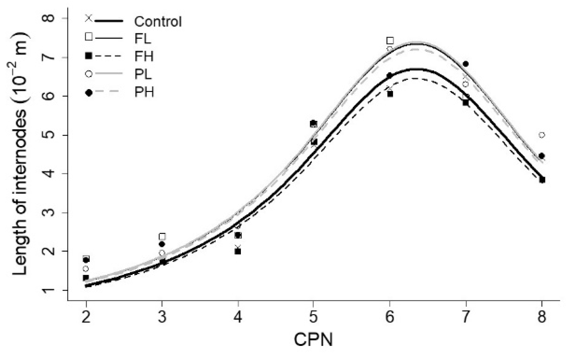
The length of internodes versus CPN revealed a lag between branches and main stems as can be seen in the example for the control treatment on Figure 2. By fitting the length of internodes of the branches as a function of CPN + 1, both lines became approximately overlapped. This means that, in length, internodes of branches were similar to the internodes of the main stem positioned one level higher in rank. Consequently, the lengths of internodes of the main stems were fitted as a function of CPN and the lengths of branches were fitted as a function of CPN + 1.
The parameterization resulting in the smallest AIC (best description of the data) for the final length of internodes was obtained when coefficient Lm was fitted to each treatment individually. Therefore, Lm was estimated for each irrigation treatment whereas xo and α were assumed to be constant over the treatments (Table 2). These results indicate that there was effect of irrigation treatment on the maximum internode length only, and not the rank at which this maximum occurred (xo), nor on the slope of the distribution curve (α). Internodes of plants in treatment FH were the shortest ones in all CPN (Figure 3). However, length of internodes of the control treatment was close to the ones at FH treatment. Overall, the estimation of length of internodes by the Cauchy-Lorentz distribution with the fitted coefficients captures most of the variation in observed data (r2 above 0.51 on Table 3. The goodness of fit markedly decreased for the irrigation deficit treatments (Table 3). Comparing the coefficient Lm confidence intervals (Table 2), the effect of the irrigation treatments on field data was also observed on fitted models. The most significantly difference was between treatments PL and FH.
From field observations, it was clear that internodes of the main stems are thicker than the internodes of branches, and fitting was therefore done separately. In both cases, there was no significant effect of water deficit on the thickness of internodes (Table S1 of Supplementary Materials).
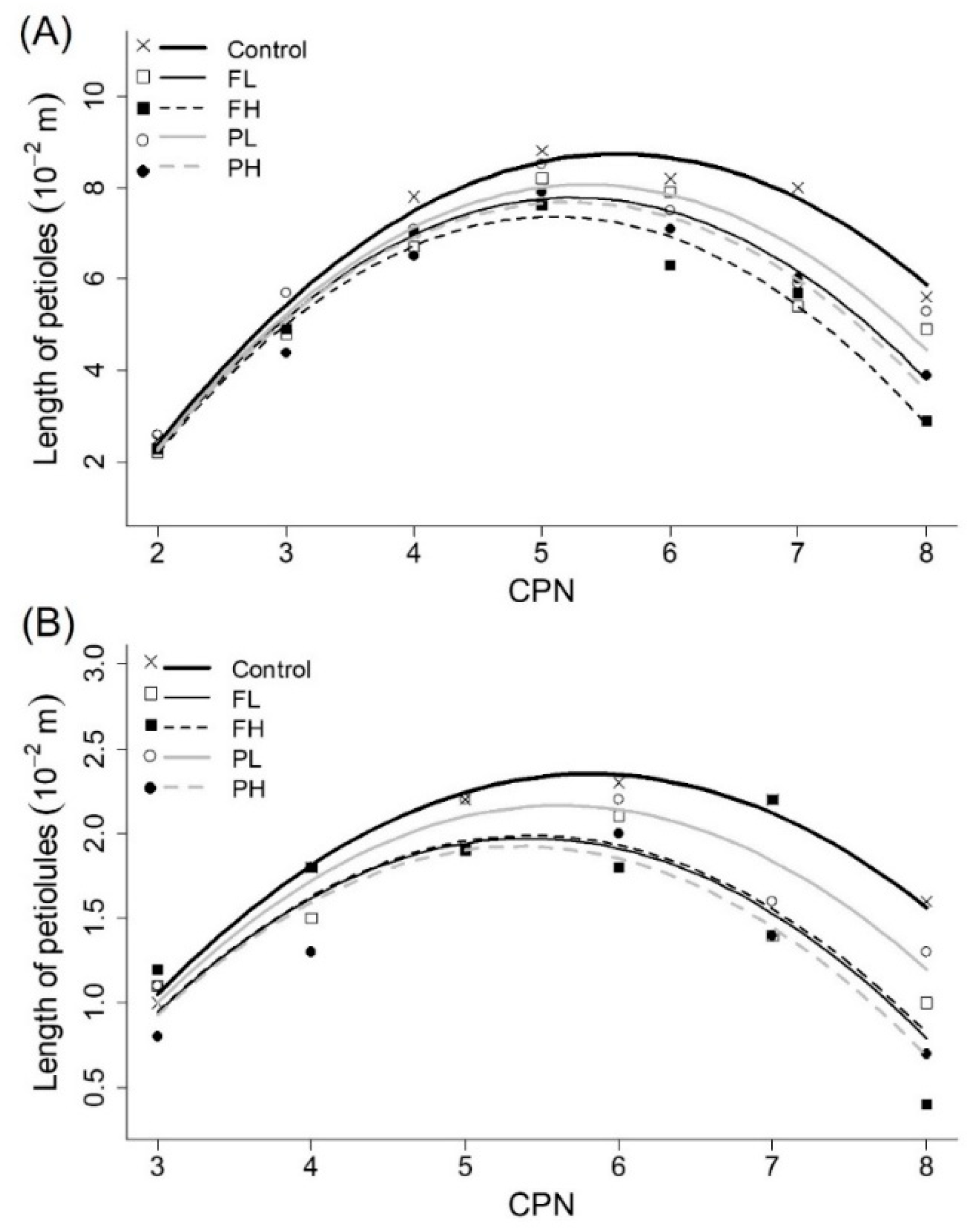
3.5. Lengths of Petioles and Petiolules
As observed for the length of internodes, the length of petioles and petiolules versus CPN for branches also showed a phase lag compared to the main stems. To represent this, the length of the main stems was represented as a function of CPN, whereas branch lengths were fitted to CPN+1. Applying dummy variables, smaller AIC values were obtained when Equation (3) fitting coefficient a was determined for each irrigation treatment (Figure 4; Table 2). This indicates a significant effect of irrigation deficit on length of petioles and petiolules. However, the quadratic model with the fitted coefficients did not capture all of the variation in the observed data of plants under water stress (r2 decreasing in most of the cases and RMSE increasing for the irrigation deficit treatments (Table 3)). Effect of the irrigation treatments was also identified on fitted models (Table 2). Model for control treatment was significantly different from models for treatments FL, FH and PH, and showed similarities with treatment PL, the less stressed one.
3.6. Size of Leaflet Blades
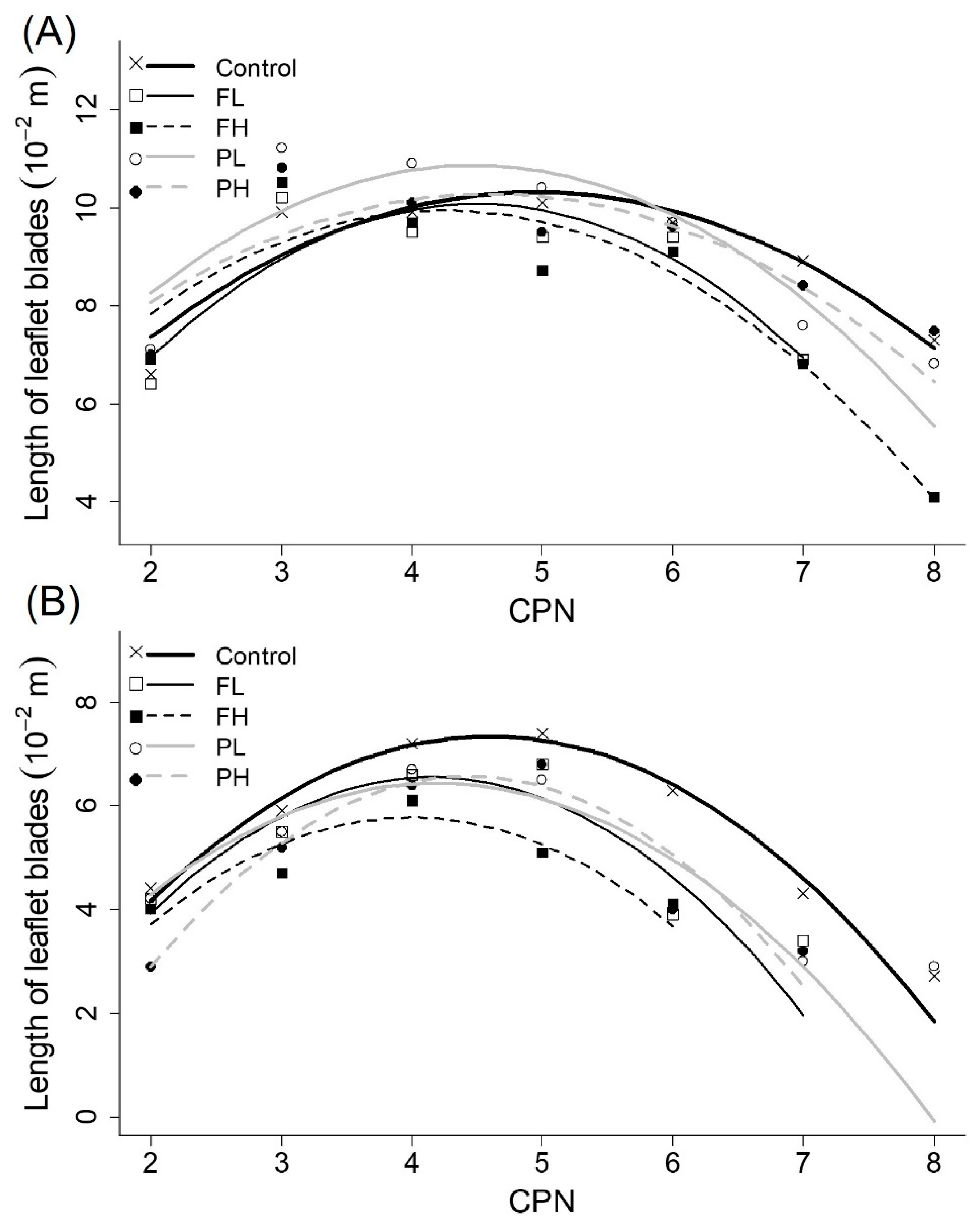
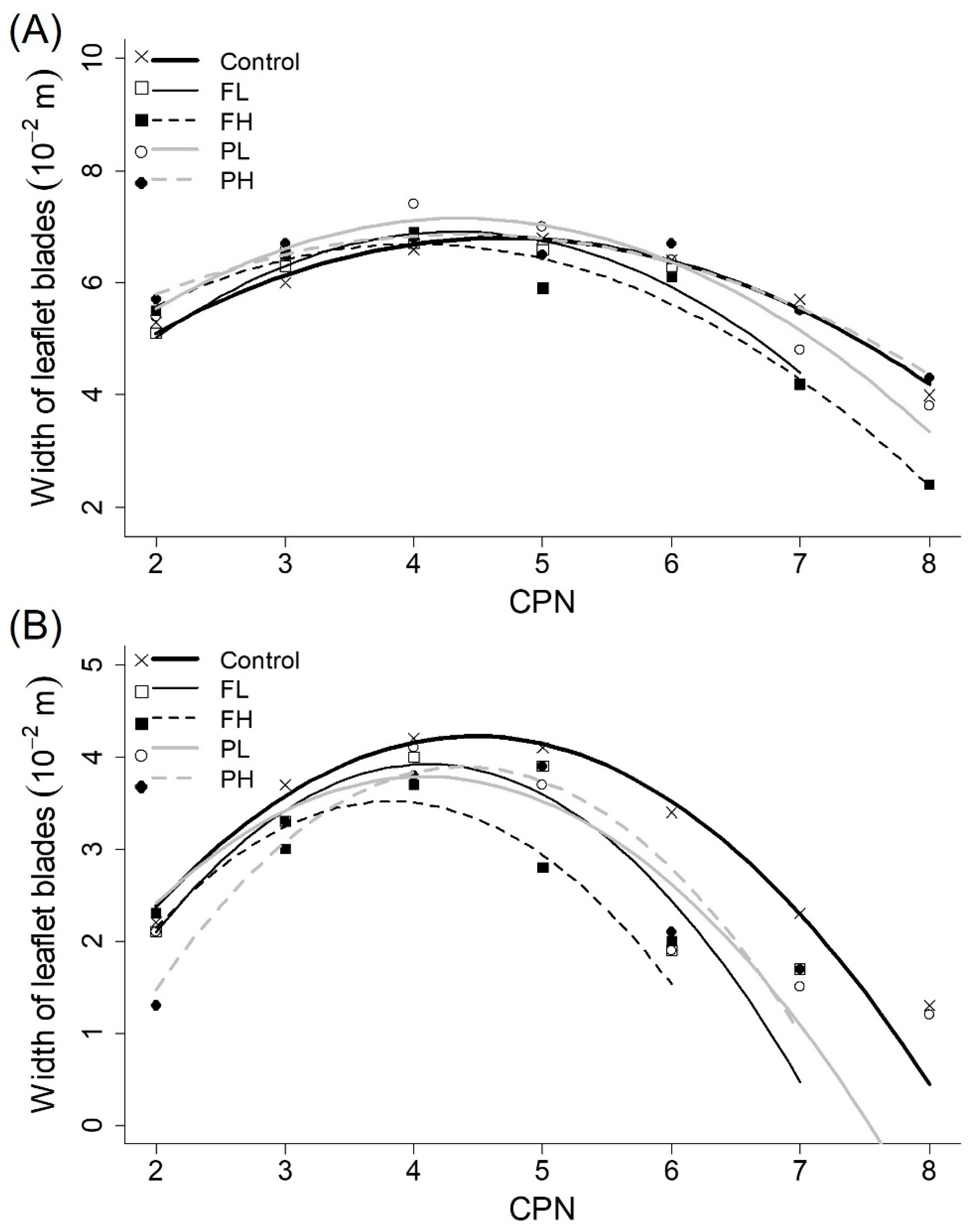
When plotting length and width of leaflet blades against CPN, two separate data groups were identified: one representing length and width on main stems and the other one grouping the leaflets on branches. In general, leaflets on branches were smaller than leaflets on main stems. Therefore, model fitting was done separately for these two groups. Smaller AIC values were obtained when all fitting coefficients were determined for each irrigation treatment individually, indicating an effect of irrigation treatments of size of leaflets (Figure 5; Figure 6; Table 2). The negative quadratic model fitted allowed to describe the sizes of leaflet blades of main stems and branches (quality of fit in Table 3). There was irrigation effect on fitted coefficients of models (Table 2). On leaflets of branches, fitted coefficients for treatments control and PL were significantly different of the ones for treatment PH. Conversely, fitted coefficients for main stems of treatments control and PH were significantly different of the ones for treatment FL. Irrigation effect was more pronounced on leaflets developed later (last CPNs) and on branches (Figure 5B and Figure 6B) than on leaves generated earlier (first CPNs) and on the main stem of plants (Figure 5A and Figure 6A).
3.7. Angles
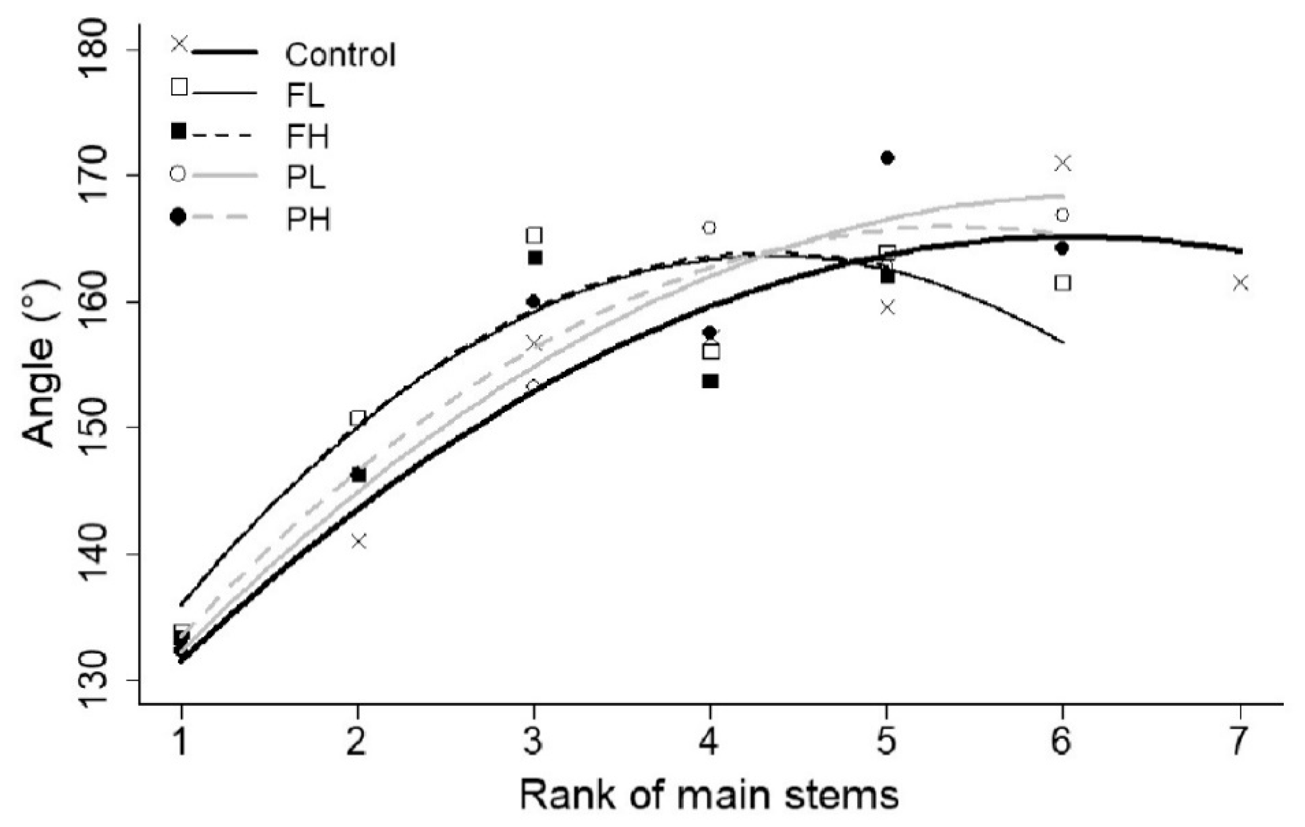
No effect of water stress was identified on angles between internodes of the main stems and a simple model with constant coefficients for all treatments describes the data (Table S1 of Supplementary Materials). Angles between first internodes of primary branches and internodes of the main originating stems were significantly affected by irrigation treatment. Those angles can be predicted by a more complex model with coefficients d and e fitted to data of each irrigation treatment individually as a function of phytomer rank number (Figure 7 and Table 2). Fitted models were able to predict the angles satisfactorily (r2 ~ 0.41 to 0.63) and lower goodness of fit was obtained for data of treatments FL and FH (Table 3). Comparing the confidence intervals of coefficients d and e (Table 2), there was a clear effect of the irrigation treatments on fitted models. The most significantly difference was between control treatment and FL and FH, showing an effect of timing of irrigation deficit on angles between first internodes of primary branches and internodes of the main originating stems. In the control treatment, angles increased with rank which makes the internodes of branches gradually more erect to give the structure of internodes a randomized distribution. On treatments FL and FH, initially the angles also increased with rank; however, from rank 4 on, angles decreased and the internodes of the branches dropped downward.
Irrigation treatments also did not significantly affect the angles between internodes and petioles and angles between petioles and petiolules. Differences were found in angles between petiolules and top leaflet blades (Table 1). High similarity was observed between the control treatment and treatments FL and PL which produced the highest grain yields. Plants of treatments FH and PH had the lowest yields and leaves pointing downward due to smaller angles.
4. Discussion
4.1. Water Applied, Evapotranspiration and Yield Traits
Irrigation deficit treatments had effect on evapotranspiration as less water was available for this process. No significant differences were observed in the final number of pods per plant in contrast to previous findings [34,57,58,59]. In a study by Barrios et al., (2005) [43], the number of pods per bean plant was reduced by 63% when no irrigation was applied during the flowering stage. In our experiment irrigation was reduced but not interrupted, and the number of pods was not significantly affected. Pods in the control treatment were significantly longer than in the other treatments, corroborating earlier work [29]. Our findings demonstrate that the final length of pods was reduced mainly as a function of total amount of water applied. The longest pods were observed in plants receiving full irrigation (control), intermediate sizes were observed in plants of both treatments receiving intermediate irrigation intensity (low deficit) and small pods were produced by plants of the most water stressed treatments (high deficit).
Grain yield and shoot biomass were significantly reduced in plants of all water deficit treatments similar to Rosales-Serna et al., (2004) [28]. Barrios et al., (2005) [43] showed grain yield to be reduced by 80% under water stress during the reproductive phase. However, effects were also due to the irrigation intensity imposed to the plants. According to Lopez et al., (1996) [59], water stress during the flowering stage in beans can reduce grain yield up to 70% depending on the level of water deficit. Furthermore, stress occurring from initial flowering to pod filling might affect pod setting and yield through a reduction of the vegetative growth of branches located in the lower nodes of the main stem [60,61]. Limiting the vegetative growth of branches may decrease the source/sink relationship between leaves and pods.
The HI of well-watered bean plants is reported to be around 0.45–0.55 [62,63], the same range as obtained in our control treatment. However, HI of bean genotypes can range between 0.32 to 0.78 [29,58,64,65]. Barrios et al., (2005) [43] showed HI to be reduced by 25.7% under water stress during reproductive phase. It is argued that there is a reduction in remobilization of N and C components from leaves to pods [58]. The comparable HI values between treatments and the control treatment of our study can be explained by the reduction of the final number of leaves given the leaf abscission observed (but not recorded) in water stressed treatments, ending in a reduced shoot biomass As a recommendation, leaf abscission should be recorded on future works to assure the precise estimation of HI.
4.2. Development and Architecture
A general effect reported in literature is the increase of phyllochron with water shortage independent of the stage of its occurrence (e.g., Gholinezhad et al., (2012) [66] for sunflower (Helianthus annuus L.), and Albert and Carberry (1993) [67] for maize (Zea mays L.)). In contrast to these findings, our results indicate that phyllochron of bean plants was more responsive to the timing when water deficit occurred than to the irrigation intensity. Comparable data on the phyllochron of common bean plants under water stress have not been reported. For flowering some data are available, which—while suggesting that flowering is a water-stress sensitive phenological stage—are inconclusive. These data report range of responses: from little response [68] to a delay in flowering only under the highest levels of water deficits [69].
Each phytomer is differentially affected according to its ontogeny and the occurrence of water stress [70]. We are, however, not aware of reports of the number of phytomers in common bean plants in literature. Boutraa and Sanders (2001) [29] reported the number of trifoliate leaves in common beans to be reduced when plants were exposed to water stress. In our case, the reduced number of leaflet blades is possibly a result of the reduced number of phytomers on FH treatment as the last phytomers produced in reproductive phase on treatments control, FL, PL and PH were not produced on plants of treatment FH.
The effect of water treatments on internodes of bean plants was significant on its lengths, instead of on its width. As the relative growth of internodes is greater in length than in width, it can be inferred that the effects were more pronounced on lengths due to the longer periods that they kept growing. However, a clear relation between the irrigation intensity and the timing of water shortage occurrence and length of internodes cannot be identified. These results partly differ from those obtained by Ku et al., (2013) [71] who showed the length of internodes to be dependent on the timing of water shortage.
Petioles and petiolules were shortened in the water treatments, especially in the high irrigation deficit. This effect is more pronounced for higher CPN values, i.e., the organs generated or still actively growing after water irrigation was reduced. Small petioles reduce the resistance of water flow from roots to leaf blades under water stress [72]. Consequently, reducing the size of petioles and petiolules is a plant survival strategy in dry conditions.
Leaf size was reduced on irrigation treatments, but a clear conclusion on the effect of the timing of water shortage occurrence and the irrigation intensity could not be addressed. The effect as more pronounced on leaflets of branches which were developed and growing later during the water shortage (last CPNs). Reduction in size of leaflet blades has a direct effect on leaf area since the total leaf area is proportional to the length and width of blades. Barrios et al., (2005) [43] found a reduction of leaf area of bean plants under water stress of the order of 10% in the main stem as compared to the reduction of 60% observed in branches.
The effect of the irrigation treatments was clear in petioles, petiolules and leaf size, but the irrigation deficit clearly affected more the petioles and petiolules than the stage of its occurrence, and a clear tendency for leaf size could not be found. This result could indicate a loss of the allometric relationship between petioles, petiolules and leaves in water deficit conditions.
The daily movement of leaves of plants under water stress (paraheliotrophism) is already described in literature for many species (e.g., soybeans [73], common bean [29,74,75] and switchgrass (Panicum virgatum) [76]). Paraheliotrophism was observed during the experiment but it was not quantitatively measured. However, our findings indicate that the shoot architecture of the water stressed bean plants (i.e., light capture) was permanently altered over the crop cycle. At the beginning of water shortage, stresses are covered by leaf and shoot movement [77]. However, at some point, irreversible changes occur on leaf slope. From our results, effect of timing of water shortage occurrence was more pronounced on angles between first internodes of primary branches and internodes of the main originating stems, significantly reducing them when water shortage started at flowering stage. On the other hand, angles between petiolules and top leaflet blades were mainly reduced due to higher irrigation deficit applied. Given that all other angles between organs were similar, plants presenting smaller angles close to main stems and at the end of phytomers have leaflet blades pointing downwards. To our knowledge, this is the first study to have explicitly quantified the long term alteration on angles of shoot architecture of common bean plants at different irrigation intensities.
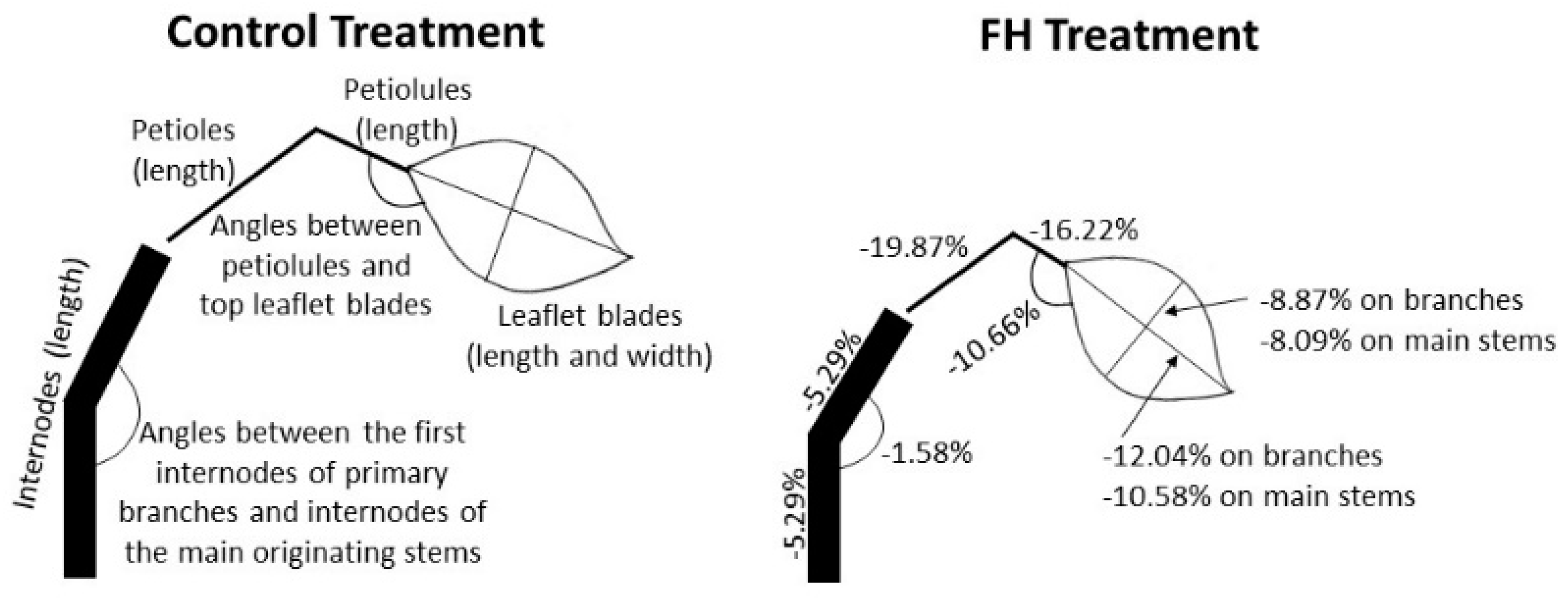
The main effects of water stress on the shoot architecture of common bean plants are summarized on Figure 8 for control treatment and treatment FH. The larger the water shortage in the flowering stage, the larger the effects. Most stressed plants were shorter, leaves were smaller and pointing downward. The appearance of consecutive leaves was slower, and the final number of phytomers and leaflets decreased. Specifically comparing plants of treatment FH to the treatment control plants (Figure 8), internodes, petioles, petiolules were shorter, length and width of leaflet blades were smaller on branches and on main stems, and the angles between internodes of primary branches and main stems (close to main stems) and between petiolules and top leaflet blades (end of phytomers) decreased.
Effect of water shortage on architecture and transpiration of common bean plants limited production. The combined effect of less available water, less transpiration with smaller leaves pointing downwards and intercepting less sunlight led to small pods, less grain yield and shoot biomass. Those effects were mainly observed in the plants in treatment FH. Plants of treatments control, FL, PL and PH had higher grain yields. However, no treatment effect was observed on the final number of pods and on the harvest index. Annual grain legumes as common beans are more sensitive to water shortage than legume plants with perennial growth habit due to the shallow and sparse root systems [78]. Soybeans and pigeon pea (Cajanus cajan (L.) Millsp.) are reported to have reduced grain yield under water shortage [43,73,79]. In these studies, water stress led to a modified architecture (e.g., smaller leaves) and changes in yield components (e.g., less grain yield and shoot biomass) similar to the ones identified in our study.
Water shortage may induce other stresses besides water stress. As a reduced part of the net radiation is consumed to evaporate water on leaves, there is more available energy to sensible heating, increasing leaf temperature. The heat stress inhibits photosynthesis, a highly temperature sensitive process [10]. In addition, water shortage decreases cell turgor pressure and induces wilting. To keep cell turgor and soil water uptake, plants adjust osmotically by synthetizing osmoprotectants. When accumulated in higher concentrations, these osmoprotectants lead to osmotic stress, affecting the physiological status and plant growth [80]. Osmotic stress also occurs when plants are grown on saline soils. The continued use of irrigation without adequate drainage management in drought-prone areas where common bean is produced in developing tropical and subtropical regions may lead to soil salinization. Preventing water stress in field production by irrigation may not be the ideal way out for avoiding alterations on common bean shoot architecture and the reduction on production as other stresses could be acting together. From our findings, bean plants are less affected by water shortages with low intensities on pod formation than on flowering. As a management strategy, farmers allow some reduction of water availability (like −30% of the plant water requirement) during the pod formation stage without significant reductions on yield.
4.3. Outlook
A dynamic and precise methodology to quantify sunlight interception of common bean plants under water limitation and its impact on physiological processes and growth is an issue for further investigation. Currently, we are lacking the tools to translate these detailed architecture measurements into the Lambert Beer extinction coefficients. A promising methodology would be the use of Functional Structural Plant (FSP) model [81,82]. In our study, FSP models could be applied to check the extent to which architectural changes caused by water stress led to reduced production. Moreover, FSP models allow a detailed investigation on distribution of sunlight capture by each organ and the time course of light interception. Describing plant architecture requires species and cultivar-specific information about when and where organs appear, as well as how they are positioned within plants. FSP models can be calibrated and tested on the basis of the relationships found in our study. Output of sunlight interception and leaf area over time produced by FSP models could be, for example, used to improve the predictive capacity of crop growth models. The observed historical crop yields are different from the results from crop models due in parts to the difficulty in representing plant architecture [5]. The combined use of architectural models could help to include second order water stress effects on crop models.
Two limitations of our study can be addressed and better explored in a future work. First, only one growing season was analyzed (2015). Data is not enough or representative to establish a strong conclusion to support findings of the effects of water shortage on common bean yield through modifications of plant shoot architecture. Moreover, only one cultivar was used (crop variety Berna). A comparison between different common bean cultivars taking into account their water shortage tolerance or sensitivity conducted in broader environmental conditions expressed in different growing seasons can support and clarify the results of our study.
Supplementary Materials
The following are available online at https://0-www-mdpi-com.brum.beds.ac.uk/2073-4395/9/3/160/s1, Table S1: Fitted coefficients for the organs which were not affected by irrigation treatments.
Author Contributions
Conceptualization, A.D., J.E., K.M. and Q.d.J.v.L.; methodology, A.D., J.E., K.M. and Q.d.J.v.L.; software, A.D., J.E. and K.M.; validation, A.D., J.E., K.M. and Q.d.J.v.L.; formal analysis, A.D., J.E. and K.M.; investigation, A.D., J.E. and K.M.; resources, A.D., J.E., K.M. and Q.d.J.v.L.; data curation, A.D., J.E., K.M. and Q.d.J.v.L.; writing—original draft preparation, A.D.; writing—review and editing, J.E., K.M. and Q.d.J.v.L.; visualization, A.D., J.E., K.M. and Q.D.J.V.L.; supervision, J.E., K.M. and Q.d.J.v.L.; project administration, A.D. and Q.d.J.v.L.; funding acquisition, K.M. and Q.d.J.v.L.
Funding
This research was funded by the São Paulo Research Foundation—FAPESP, Brazil (projects 2012/09316-8 and 2013/19374-8), and the Soil Physics and Land Management Group of Wageningen University and Research Centre, The Netherlands.
Acknowledgments
The authors are grateful for the support of Jacob C. Douma and Junqi Zhu, and for the technical support during the experiment of the Nergena/Unifarm group, especially Rinie Verwoert and Rohan van Genderen.
Conflicts of Interest
The authors declare no conflict of interest.
Appendix A. Dummy-Variable Regression Method
Applying dummy variables in the models indicates whether a coefficient can represent the entire dataset of all treatments or whether it must be fitted to each treatment separately due to the treatment effect. To include dummy variables in a model, they should be converted to continuous variables that assume only two values, 0 or 1. For each coefficient of a model with j categories, j−1 dummy variables are needed. In this specific case, j is equal to 5 representing the number of irrigation treatments, and four dummy variables are needed. For the Cauchy-Lorentz distribution model (Equation (1)) with three coefficients (Lm, xo and α), the dummy variables are d1, d2, d3 and d4 with values of 0 or 1 and the coefficients Lm,1…Lm,4, xo,1…xo,4, and α1…α4:
then indicates how different the effects of water stress treatments are from those of the reference (control), i.e., the coefficients for dummy variables express the differential effects of each category compared to a reference category (in which all dummy variables are equal to zero). Some types of models were tested differing in the number of dummy variables used. In the so-called extended model, dummy variables were applied to all model coefficients and all of them were fitted. In the simplest case, no dummy variables were applied and only Lm, xo and α were fitted. Combinations of coefficients were also analyzed. For example, in a model Lm-α, the dummy variables were applied to these two coefficients and were not applied to coefficient xo.
References
- Manschadi, A.M.; Christopher, J.; Voil, P.D.; Hammer, G.L. The role of root architectural traits in adaptation of wheat to water-limited environments. Func. Plant Biol. 2006, 33, 823–837. [Google Scholar] [CrossRef] [Green Version]
- Atta, B.M.; Mahmood, T.; Trethowan, R.M. Relationship between root morphology and grain yield of wheat in north-western NSW, Australia. Aust. J. Crop Sci. 2013, 7, 2108–2115. [Google Scholar]
- UNDP. Reducing Disaster Risk: A Challenge for Development. A Global Report. Available online: http://www.undp.org/cpr/whats_new/rdr_english.pdf (accessed on 14 January 2019).
- Helmer, M.; Hilhorst, D. Natural disasters and climate change. Disasters 2006, 30, 1–4. [Google Scholar] [CrossRef]
- Li, Y.; Ye, W.; Wang, M.; Yan, X. Climate change and drought: A risk assessment of crop-yield impacts. Climate Res. 2009, 39, 31–46. [Google Scholar] [CrossRef]
- IPCC. Summary for policymakers. In Climate Change 2014: Impacts, Adaptation, and Vulnerability. Part A: Global and Sectoral Aspects. Contribution of Working Group II to the Fifth Assessment Report of the Intergovernmental Panel on Climate Change; Field, C.B., Barros, V.R., Dokken, D.J., Mach, K.J., Mastrandrea, M.D., Bilir, T.E., Chatterjee, M., Ebi, K.L., Estrada, Y.O., Genova, R.C., et al., Eds.; Cambridge University Press: Cambridge, UK, 2014; pp. 1–32. [Google Scholar]
- Dai, A.; Trenberth, K.E.; Qian, T. A global data set of Palmer Drought Severity Index for 1870–2002: Relationship with soil moisture and effects of surface warming. J. Hydrometeorol. 2004, 5, 1117–1130. [Google Scholar] [CrossRef]
- Rosegrant, M.W.; Cline, S.A. Global food security: Challenges and policies. Science 2003, 302, 1917–1919. [Google Scholar] [CrossRef]
- Ericksen, P.J. Conceptualizing food systems for global environmental change research. Glob. Environ. Chang. 2008, 18, 234–245. [Google Scholar] [CrossRef]
- Taiz, L.; Zeiger, E. Plant Physiology, 5th ed.; Sinauer Associates: Sunderland, UK, 2010; 782p. [Google Scholar]
- Monclus, R.; Dreyer, E.; Villar, M.; Delmotte, F.M.; Delay, D.; Pettit, J.M.; Barbaroux, C.; Thiec, D.; Brechet, C.; Brignolas, F. Impact of drought on productivity and water use efficiency in 29 genotypes of Populus deltoides x Populus nigra. New Phytol. 2006, 169, 765–777. [Google Scholar] [CrossRef]
- Haldimann, P.; Galle, A.; Feller, U. Impact of an exceptionally hot dry summer on photosynthetic traits in oak (Quercus pubescens) leaves. Tree Physiol. 2008, 28, 785–795. [Google Scholar] [CrossRef]
- Ruiz-Ramos, M.; Mínguez, M.I. ALAMEDA, a structural-functional model for faba bean crops: Morphological parameterization and verification. Ann. Bot. 2006, 97, 377–388. [Google Scholar] [CrossRef]
- Roujean, J.-L. A tractable physical model of shortwave radiation interception by vegetative canopies. J. Geophys. Res. 1996, 101, 9523–9532. [Google Scholar] [CrossRef]
- Archontoulis, S.V.; Vos, J.; Yin, X.; Bastiaans, L.; Danalatos, N.G.; Struik, P.C. Temporal dynamics of light and nitrogen distributions in canopies of sunflower, kenaf and cynara. Field Crops Res. 2011, 122, 186–198. [Google Scholar] [CrossRef]
- Atti, S.; Bonnel, R.; Prasher, S.; Smith, D.L. Response of soybean {Glycine max (L.) merr.} under chronic water deficit to LCO application during flowering and pod filling. Irrig. Drain. 2005, 54, 15–30. [Google Scholar] [CrossRef]
- Graham, P.H.; Vance, C.P. Legumes: Importance and constraints to greater use. Plant Physiol. 2003, 131, 872–877. [Google Scholar] [CrossRef]
- Mitchell, D.C.; Lawrence, F.R.; Hartman, T.J.; Curran, J.M. Consumption of dry beans, peas, and lentils could improve diet quality in the US population. J. Am. Diet. Ass. 2009, 109, 909–913. [Google Scholar] [CrossRef]
- Pachico, D. Trends in world common bean production. In Bean Production Problems in the Tropics; Schwartz, H.F., Pastor-Corrales, M.A., Eds.; International Center for Tropical Agriculture (CIAT): Cali, Colombia, 1989; pp. 1–8. [Google Scholar]
- Ramirez-Vallejo, P.; Kelly, I.D. Traits related to drought resistance in common bean. Euphytica 1998, 99, 127–136. [Google Scholar] [CrossRef]
- Broughton, W.J.; Hernandez, G.; Blair, M.; Beebe, S.; Gepts, P.; Vanderleyden, J. Beans (Phaseolus spp.)-model food legumes. Plant Soil 2003, 252, 55–128. [Google Scholar] [CrossRef]
- Petry, N.; Boy, E.; Worth, J.P.; Hurrel, R. The potential of the Common Bean (Phaseolus vulgaris) as a vehicle for iron biofortification. Nutrients 2015, 7, 1144–1173. [Google Scholar] [CrossRef] [PubMed]
- van Schoonhoven, A.; Voysest, O. Common beans in Latin America and their constraints. In Bean Production Problems in the Tropics, 2nd ed.; Schwartz, H.F., Pastor-Corrales, M.A., Eds.; International Center for Tropical Agriculture (CIAT): Cali, Colombia, 1989; pp. 33–37. [Google Scholar]
- Shellie-Dessert, K.; Bliss, F. Genetic improvement of food quality factors. In Common Beans: Research for Crop Improvement; van Schoonhoven, A., Voyses, O., Eds.; CAB International in association with International Center for Tropical Agriculture (CIAT): Cali, Colombia, 1991; pp. 649–679. [Google Scholar]
- Back, A.J. Irrigation of bean culture in the South of Santa Catarina state–Brazil. Rev. Tec. Amb. 2001, 7, 35–44. [Google Scholar]
- Wallace, D.H. Adaptation of Phaseolus to different environments. In Advances in Legume Science; Summerfield, R.J., Bunting, A.H., Eds.; Royal Botanic Gardens: Kew, UK, 1980; pp. 349–357. [Google Scholar]
- Halterlein, A.J. Bean. In Crop Water Relations; Teare, I.D., Peet, M.M., Eds.; Willey & Sons: New York, NY, USA, 1983; pp. 157–185. [Google Scholar]
- Rosales-Serna, R.; Kohashi-Shibata, J.; Acosta-Gallegos, J.A.; Trejo-Lopez, C.; Ortiz-Cereceres, J.; Kelly, J.D. Biomass distribution, maturity acceleration and yield in drought stressed common bean cultivars. Field Crops Res. 2004, 85, 203–211. [Google Scholar] [CrossRef]
- Boutraa, T.; Sanders, F.E. Effects of interactions of moisture regime and nutrient addition on nodulation and carbon partitioning in two cultivars of bean (Phaseolus vulgaris L.). J. Agron. Crop Sci. 2001, 186, 229–237. [Google Scholar] [CrossRef]
- Miller, D.E.; Burke, D.W. Response of dry beans to daily deficit sprinkler irrigation. Agron. J. 1983, 75, 775–778. [Google Scholar] [CrossRef]
- Silveira, P.M.; Steinmetz, S.; Guimarães, C.M.; Aidar, H.; Carvalho, J.R.P. Frequency and levels of irrigation in dry beans during winter season. Pesq. Agropec. Bras. 1984, 19, 219–223. [Google Scholar]
- Doorenbos, J.; Pruitt, W.O. Crop Water Requirements. Irrigation and Drainage Paper; n. 24; Food and Agriculture Organization of The United Nations: Rome, Italy, 1976; 189p. [Google Scholar]
- Costa-Franca, M.G.; Thi, A.T.; Pimentel, C.; Pereyra, R.O.; Zuily-Fodil, Y.; Laffray, D. Differences in growth and water relations among Phaseolus vulgaris cultivars in response to induced drought stress. Environ. Exp. Bot. 2000, 43, 227–237. [Google Scholar] [CrossRef]
- Acosta-Gallegos, J.A.; Adams, M.W. Plant traits and yield stability of dry bean (Phaseolus vulgaris L.) cultivars under drought stress. J. Agric. Sci. 1991, 117, 213–219. [Google Scholar] [CrossRef]
- Adams, M.W.; Coyne, D.P.; Davis, J.H.C.; Graham, P.H.; Francis, C.A. Common bean (Phaseolus vulgaris L.). In Grain Legume Crops; Summerfield, R.J., Roberts, E.H., Eds.; Collins: London, UK, 1985; pp. 433–476. [Google Scholar]
- Xia, M.Z. Effect of soil drought during the generative development phase on seed yield and nutrient uptake of faba bean (Vicia faba L.). Aust. J. Agric. Res. 1997, 48, 447–451. [Google Scholar] [CrossRef]
- Loss, S.P.; Siddique, K.H.M.; Tennant, D. Adaptation of faba bean (Vicia faba L.) to dryland Mediterranean-type environments I. Seed yield and yield components. Field Crops Res. 1997, 52, 17–28. [Google Scholar] [CrossRef]
- Mwanamwenge, J.; Loss, S.P.; Siddique, K.H.M.; Cocks, P.S. Effect of water stress during floral initiation, flowering and podding on the growth and yield of faba bean (Vicia faba L.). Eur. J. Agron. 1999, 11, 1–11. [Google Scholar] [CrossRef]
- Doorenbos, J.; Kassam, A.H. Yield Response to Water. Irrigation and Drainage Paper; n. 33; Food and Agriculture Organization of The United Nations: Rome, Italy, 1979; 306p. [Google Scholar]
- Pardossi, A.; Vernieri, P.; Tognoni, T. Involvement of abscisic acid in regulating water status in Phaseolus vulgaris L. during chilling. Plant Physiol. 1992, 100, 1243–1250. [Google Scholar] [CrossRef] [PubMed]
- Comstock, J.; Ehleringer, J. Stomatal response to humidity in common bean (Phaseolus vulgaris): Implications for maximum transpiration rate, water-use efficiency and productivity. Aust. J. Plant Physiol. 1993, 20, 669–691. [Google Scholar] [CrossRef]
- Njoka, E.M.; Muraya, M.M.; Okumu, M. The influences of plant density on yield and yield components of common beans (Phaseolus vulgaris L.). Agric. Trop. Subtrop. 2005, 38, 22–29. [Google Scholar]
- Barrios, A.N.; Hoogenboom, G.; Nesmith, D.S. Drought stress and the distribution of vegetative and reproductive traits of a bean cultivar. Scientia Agric. 2005, 62, 18–22. [Google Scholar] [CrossRef]
- Silva, A.O.; Lima, E.A.; Fidelis Filho, J.; Nóbrega, J.Q. Dry matter accumulation of beans grown in different densities in Lagoa Seca-PB. In Proceedings of the XIV Brazilian Conference of Meteorology, Florianópolis, Brazil, 27 November–1 December 2006. [Google Scholar]
- Steeves, T.A.; Sussex, I.M. Patterns in Plant Development, 2nd ed.; Cambridge University Press: New York, NY, USA, 1989; 408p. [Google Scholar]
- McMaster, G.S. Phytomers, phyllochrons, phenology and temperate cereal development. J. Agric. Sci. 2005, 143, 137–150. [Google Scholar] [CrossRef]
- Brossinger, G. Segments (Phytomers). In Handbook of Plant Science; Roberts, K., Ed.; Willey & Sons: Chichester, UK, 2007; pp. 200–202. [Google Scholar]
- Barbosa Machado Neto, N.; Prioli, M.R.; Gatti, A.B.; Mendes Cardoso, V.J. Temperature effects on seed germination in races of common beans (Phaseolus vulgaris L.). Acta Scient. Agron. 2006, 28, 155–164. [Google Scholar]
- Abramoff, M.D.; Magalhaes, P.J.; Ram, S.J. Image processing with ImageJ. Biophotonics Intern. 2004, 11, 36–42. [Google Scholar]
- Buck-Sorlin, G.H. L-system model of the vegetative growth of winter barley. In Proceedings of the Fifth German Workshop on Artificial Life, Lübek, Germany, 18–20 March 2002; Polani, D., Kim, J., Martinez, T., Eds.; pp. 53–64. [Google Scholar]
- R Development and Core Team. An Introduction to R. Notes on R: A Programming Environment for Data Analysis and Graphics Version 3.1.1; R Foundation for Statistical Computing: Vienna, Austria, 2014; 105p. [Google Scholar]
- Quinn, G.; Keough, M. Experimental Design and Data Analysis for Biologists; Cambridge University Press: Cambridge, UK, 2002; 553p. [Google Scholar]
- Carvalho, I.R.; Korcelski, C.; Pelissari, G.; Hanus, A.D.; Rosa, G.M. Water demand of crop agronomic interest. Enciclop. Biosfera 2013, 9, 969–985. [Google Scholar]
- Bergamaschi, G.; Vieira, H.J.; Libardi, P.L.; Ometto, J.C.; Angelocci, L.R. Water deficit in common bean. III. Maximum crop evapotranspiration and its relationship with evapotranspiration by the Penman method and “Class A” Pan evaporation. Pesq. Agropec. Bras. 1989, 24, 387–392. [Google Scholar]
- Santos, R.Z.; André, R.G.B. Water use for bean crop in different growth stages. Pesq. Agropec. Bras. 1992, 27, 543–548. [Google Scholar]
- Saxena, C.M.; Singh, B.K. Effect of supplementary irrigation during reproductive growth on winter and spring chickpea (Cicer arietinum) in a Mediterranean environment. J. Agric. Sci. 1990, 114, 285–293. [Google Scholar] [CrossRef]
- Acosta-Gallegos, J.A.; Shibata, J.K. Effect of water stress on growth and yield of indeterminate dry-bean (Phaseolus vulgaris) cultivars. Field Crops Res. 1989, 20, 81–93. [Google Scholar] [CrossRef]
- Castellanos, J.Z.; Pena-Cabriales, J.J.; Acosta-Gallegos, J.A. 15N-determined dinitrogen fixation capacity of common bean (Phaseolus vulgaris L.) cultivars under water stress. J. Agric. Sci. 1996, 126, 327–333. [Google Scholar] [CrossRef]
- Lopez, F.B.; Johansen, C.; Chauhan, Y.S. Effect of timing of drought stress on phenology, yield and yield components of a short-duration pigeon pea. J. Agron. Crop Sci. 1996, 177, 311–320. [Google Scholar] [CrossRef]
- Board, J.E.; Harville, B.G. Late-planted soybean yield response to reproductive source/sink stress. Crop Sci. 1998, 38, 763–771. [Google Scholar] [CrossRef]
- Linkemer, G.; Board, J.E.; Musgrave, M.E. Water logging effects on growth and yield components in late planted soybeans. Crop Sci. 1998, 38, 1576–1584. [Google Scholar] [CrossRef] [PubMed]
- Scully, B.T.; Wallace, D.H. Variation in and relationship of biomass, growth rate, harvest index, and phenology to yield of common bean. J. Am. Soc. Hortic. Sci. 1990, 115, 218–225. [Google Scholar] [CrossRef]
- Araújo, A.P.; Teixeira, M.G. Ontogenetic variations on absorption and utilization of phosphorus in common bean cultivars under biological nitrogen fixation. Plant Soil 2000, 225, 1–10. [Google Scholar] [CrossRef]
- Foster, E.F.; Pajarito, A.J.A.; Acosta, G. Moisture stress impact on N partitioning, N remobilization and N-use efficiency in beans (Phaseolus vulgaris L.). J. Agric. Sci. 1995, 124, 27–37. [Google Scholar] [CrossRef]
- Acosta-Díaz, E.; Acosta-Gallegos, J.A.; Trejo-López, C.; Padilla-Ramírez, J.S.; Amador-Ramírez, M.D. Adaptation traits in dry bean cultivars grown under drought stress. Agric. Téc. Méx. 2009, 4, 416–425. [Google Scholar]
- Gholinezhad, E.; Aynaband, A.; Ghorthapeh, A.H.; Noormohamadi, G.; Bernousi, I. Study of the effect of drought stress on grain yield, quality traits, phyllochron and leaf appearance rate of sunflower hybrid Iroflor at different levels of nitrogen and plant population. Am.-Eurasian J. Agric. 2012, 12, 306–314. [Google Scholar]
- Albert, D.G.; Carberry, P.S. The influence of water deficit prior to tassel initiation on maize growth, development and yield. Field Crops Res. 1993, 31, 55–59. [Google Scholar] [CrossRef]
- White, J.W.; Izquierdo, J. Physiology of yield potential and stress tolerance. In Common Beans: Research for Crop Improvement; Schoonhoven, A., Voysest, O., Eds.; C. A. B. International: Wallingford, UK, 1991; pp. 287–382. [Google Scholar]
- Robins, J.S.; Domingo, C.E. Moisture deficits in relation to the growth and development of dry beans. Agron. J. 1956, 48, 67–70. [Google Scholar] [CrossRef]
- Kohashi-Shibata, J.; Galván, M.T.; García, A.E.; Yánez, P.J.; Martínez, E.V.; Ruiz, L.P. Water stress effect on the growth of phytomers in common bean (Phaseolus vulgaris L.). Agric. Téc. Méx. 2002, 28, 65–75. [Google Scholar]
- Ku, Y.S.; Au-Yeung, W.K.; Yung, Y.L.; Li, M.W.; Wen, C.Q.; Liu, X.; Lam, H.M. Drought stress and tolerance in soybean. In A Comprehensive Survey of International Soybean Research—Genetics, Physiology, Agronomy and Nitrogen Relationships; Board, J.E., Ed.; InTech: Rijeka, Croatia, 2013; pp. 209–237. [Google Scholar]
- Du, N.; Guo, W.; Zhang, X. Morphological and physiological responses of Vitex negundo L. var. heterophylla (Franch.) Rehd. to drought stress. Acta Physiol. Plant. 2010, 32, 839–848. [Google Scholar] [CrossRef]
- Oosterhuis, D.M.; Walker, S.; Eastham, J. Soybean leaflet movements as an indicator of crop water stress. Crop Sci. 1985, 25, 1101–1106. [Google Scholar] [CrossRef]
- Yu, F.; Berg, V.A. Control of paraheliotropism in two Phaseolus species. Plant Physiol. 1994, 106, 1567–1573. [Google Scholar] [CrossRef]
- Pastenes, C.; Pimentel, P.; Lillo, J. Leaf movements and photoinhibition in relation to water stress in field-grown beans. J. Exp. Bot. 2004, 56, 425–433. [Google Scholar] [CrossRef] [PubMed] [Green Version]
- Xu, B.; Sathitsuksanoh, N.; Tang, Y.H.; Udvardi, M.K.; Zhang, J.Y.; Shen, Z.X.; Balota, M.; Harich, K.; Zhang, Y.H.P.; Zhao, B.Y. Overexpression of AtLov1 in switchgrass alters plant architecture, lignin content, and flowering time. PLoS ONE 2012, 7, e47399. [Google Scholar] [CrossRef] [PubMed]
- Chávez, R.O.; Clevers, J.G.P.W.; Herold, M.; Ortiz, M.; Acevedo, E. Modelling the spectral response of the desert tree Prosopis tamarugo to water stress. Int. J. Appl. Earth Obs. Geoinf. 2013, 21, 53–65. [Google Scholar] [CrossRef]
- Farooq, M.; Gogoi, N.; Barthakur, S.; Baroowa, B.; Bharadwaj, N.; Alghamdi, S.S.; Siddique, K.H.M. Drought stress in grain legumes during reproduction and grain filling. J. Agron. Crop Sci. 2017, 203, 81–102. [Google Scholar] [CrossRef]
- Desclaux, D.; Huynh, T.T.; Roumet, P. Identification of soybean plant characteristics that indicate the timing of drought stress. Crop Sci. 2000, 40, 716–722. [Google Scholar] [CrossRef]
- Ueda, A.; Kathiresan, A.; Inada, M.; Narita, Y.; Nakamura, T.; Shi, W.; Takabe, T.; Benett, J. Osmotic stress in barley regulates expression of a different set of genes than salt stress does. J. Exp. Bot. 2009, 55, 2213–2218. [Google Scholar] [CrossRef] [PubMed]
- Vos, J.; Evers, J.B.; Buck-Sorlin, G.H.; Andrieu, B.; Chelle, M.; de Visser, P.H.B. Functional-structural plant modeling: A new versatile tool in crop science. J. Exp. Bot. 2010, 61, 2101–2115. [Google Scholar] [CrossRef] [PubMed]
- Evers, J.B. Simulating crop growth and development using functional-structural plant modeling. In Canopy Photosynthesis: From Basic to Applications; Hikosaka, K., Niinemets, U., Anten, N.P.R., Eds.; Springer: Dordrecht, The Netherlands, 2016; pp. 219–236. [Google Scholar]
Figure 1.
Schematic figure of part of a bean plant with the organs (sizes and angles) measured in this study. Dashed line indicates the structures of a phytomer: lateral buds, an internode, a node and a trifoliate leaf. CPN is the cumulative phytomer number (i.e., the phytomer number counted from the first phytomer of the main stem) and Rank is the phytomer number counted from the bottom of the shoot it belongs to (figure not to scale).

Figure 2.
Average length of internodes (10−2 m) of main stems and branches as a function of CPN and branches as a function CPN + 1 for the control treatment.
Figure 2.
Average length of internodes (10−2 m) of main stems and branches as a function of CPN and branches as a function CPN + 1 for the control treatment.

Figure 3.
Average observed final length of internodes (10−2 m) (symbols) and fitted Cauchy-Lorentz distribution (lines) as a function of CPN for all irrigation treatments.
Figure 3.
Average observed final length of internodes (10−2 m) (symbols) and fitted Cauchy-Lorentz distribution (lines) as a function of CPN for all irrigation treatments.

Figure 4.
Average observed final length of (A) petioles and (B) petiolules (10−2 m) (symbols) and fitted quadratic model (lines) as a function of CPN for all irrigation treatments.
Figure 4.
Average observed final length of (A) petioles and (B) petiolules (10−2 m) (symbols) and fitted quadratic model (lines) as a function of CPN for all irrigation treatments.

Figure 5.
Average observed final length of leaflet blades of (A) the main stems and (B) branches (10−2 m) (symbols) and fitted quadratic model (lines) as a function of CPN for all irrigation treatments.
Figure 5.
Average observed final length of leaflet blades of (A) the main stems and (B) branches (10−2 m) (symbols) and fitted quadratic model (lines) as a function of CPN for all irrigation treatments.

Figure 6.
Average observed final width of leaflet blades of (A) the main stems and (B) branches (10−2 m) (symbols) and fitted quadratic model (lines) as a function of CPN for all irrigation treatments.
Figure 6.
Average observed final width of leaflet blades of (A) the main stems and (B) branches (10−2 m) (symbols) and fitted quadratic model (lines) as a function of CPN for all irrigation treatments.

Figure 7.
Average observed final angles between first internodes of primary branches and internodes of the main originating stems (°) (symbols), fitted quadratic model (lines) as a function of the phytomer rank number of main stems for all irrigation treatments.
Figure 7.
Average observed final angles between first internodes of primary branches and internodes of the main originating stems (°) (symbols), fitted quadratic model (lines) as a function of the phytomer rank number of main stems for all irrigation treatments.

Figure 8.
Effect of water treatments on organ sizes of treatments control and FH (length and width of leaflet blades, length of petioles and petiolules, length of internodes, angles between the first internode of primary branches and internodes of the main originating stems, and angles between petiolules and top leaflet blades) (figure not to scale).


Table 1.
Total water applied (mm), average evapotranspiration (mm d−1), grain yield (g plant−1), shoot biomass (g plant−1), harvest index HI, final number of pods per plant, average length of pods (m), phyllochron (°Cd) on branches 2.1 and 2.2 (branches 1 and 2 generated on second rank of main stems), final number of phytomers, final number of leaflet blades and angles between petiolules and top leaflet blades (°) (± standard error) for all treatments. FL: flowering stage, low deficit; FH: flowering stage, high deficit; PL: pod formation state, low deficit; PH: pod formation stage, high deficit.
| Variable | Treatment | |||||||||
|---|---|---|---|---|---|---|---|---|---|---|
| Control | FL | FH | PL | PH | ||||||
| Water applied (mm) | 383 | 308 | 259 | 316 | 272 | |||||
| Evapotranspiration (mm d−1) | 4.89 ± 0.22 1 | a | 3.99 ± 0.12 | b | 3.33 ± 0.11 | c | 4.11 ± 0.14 | b | 3.54 ± 0.13 | c |
| Grain yield (g plant−1) | 12.89 ± 0.34 | a | 9.31 ± 0.25 | c | 7.16 ± 0.31 | d | 11.09 ± 0.31 | b | 8.16 ± 0.40 | cd |
| Shoot biomass (g plant−1) | 24.95 ± 1.23 | a | 16.84 ± 0.80 | c | 13.18 ± 0.67 | d | 19.42 ± 1.17 | b | 15.52 ± 0.47 | cd |
| Harvest index (HI) | 0.52 ± 0.03 | a | 0.56 ± 0.03 | a | 0.55 ± 0.03 | a | 0.58 ± 0.04 | a | 0.53 ± 0.04 | a |
| Number of pods per plant | 39.41 ± 1.23 | a | 41.24 ± 1.81 | a | 33.04 ± 2.97 | a | 37.49 ± 2.03 | a | 40.87 ± 1.56 | a |
| Length of pods (10−2 m) | 9.86 ± 1.91 | a | 8.12 ± 2.18 | b | 7.74 ± 2.26 | c | 8.98 ± 2.14 | b | 7.35 ± 2.21 | c |
| Phyllochron on branch 2.1 (°Cd) | 67.91 ± 4.15 | a | 91.81 ± 1.23 | b | 91.44 ± 1.02 | b | 68.94 ± 1.22 | a | 71.91 ± 1.43 | a |
| Phyllochron on branch 2.2 (°Cd) | 66.77 ± 6.56 | a | 91.86 ± 0.85 | b | 91.34 ± 1.25 | b | 76.62 ± 3.64 | a | 76.37 ± 4.16 | a |
| Final number of phytomers | 21.03 ± 1.08 | a | 17.84 ± 1.25 | ab | 14.21 ± 1.66 | b | 20.49 ± 1.07 | a | 21.45 ± 0.79 | a |
| Final number of leaflet blades | 55.03 ± 3.71 | a | 44.44 ± 4.85 | ab | 33.21 ± 2.82 | b | 52.81 ± 4.67 | a | 52.08 ± 1.23 | a |
| Angles—petiolules and top leaflet blades (°) | 135.22 ± 1.72 | a | 134.07 ± 2.86 | a | 120.89 ± 4.01 | b | 130.63 ± 2.29 | a | 126.62 ± 1.72 | b |
1 Values in the same line followed by the same letter do not significantly differ (Tukey test at 5% probability).
Table 2.
Final values of fitted coefficients of models (± standard error) for all irrigation treatments. FL: flowering stage, low deficit; FH: flowering stage, high deficit; PL: pod formation state, low deficit; PH: pod formation stage, high deficit.
Table 2.
Final values of fitted coefficients of models (± standard error) for all irrigation treatments. FL: flowering stage, low deficit; FH: flowering stage, high deficit; PL: pod formation state, low deficit; PH: pod formation stage, high deficit.
| Variable | Fitted Coefficients | Treatment | |||||||||
|---|---|---|---|---|---|---|---|---|---|---|---|
| Control | FL | FH | PL | PH | |||||||
| Length of internodes | Lm (10−2 m) | 6.71 ± 0.14 1 | bc | 7.35 ± 0.22 | ab | 6.47 ± 0.18 | c | 7.40 ± 0.18 | a | 7.21 ± 0.17 | abc |
| xo | 6.35 ± 0.04 | ||||||||||
| α | 1.95 ± 0.07 | ||||||||||
| Length of petioles | a (10−3 m) | −4.91 ± 0.05 | a | −5.24 ± 0.07 | b | −5.39 ± 0.09 | b | −5.14 ± 0.06 | ab | −5.28 ± 0.07 | b |
| b (10−2 m) | 5.50 ± 0.30 | ||||||||||
| c (10−2 m) | −6.63 ± 0.7 | ||||||||||
| Length of petiolules | a (10−3 m) | −1.64 ± 0.02 | a | −1.76 ± 0.02 | b | −1.76 ± 0.03 | b | −1.70 ± 0.02 | ab | −1.78 ± 0.02 | b |
| b (10−2 m) | 1.91 ± 0.18 | ||||||||||
| c (10−2 m) | −3.20 ± 0.49 | ||||||||||
| Length of leaflet blades (main stems) | a (10−3 m) | −3.41 ± 0.20 | a | −5.01 ± 0.37 | b | −4.18 ± 0.33 | ab | −4.26 ± 030 | ab | −3.30 ± 0.41 | a |
| b (10−2 m) | 3.37 ± 0.20 | b | 4.50 ± 0.34 | a | 3.55 ± 0.31 | ab | 3.81 ± 030 | ab | 3.03 ± 0.39 | b | |
| c (10−2 m) | 1.98 ± 0.47 | ab | −0.05 ± 0.73 | b | 2.41 ± 0.69 | ab | 2.34 ± 0.68 | ab | 3.32 ± 0.85 | a | |
| Length of leaflet blades (branches) | a (10−3 m) | −4.74 ± 0.35 | a | −5.66 ± 0.43 | ab | −5.20 ± 1.00 | ab | −4.48 ± 0.41 | a | −6.19 ± 0.38 | b |
| b (10−2 m) | 4.35 ± 0.32 | ab | 4.70 ± 0.37 | ab | 4.15 ± 0.76 | ab | 3.75 ± 0.38 | b | 5.49 ± 0.33 | a | |
| c (10−2 m) | −2.64 ± 0.73 | a | −3.22 ± 0.77 | ab | −2.50 ± 1.37 | ab | −1.42 ± 0.83 | a | −5.62 ± 0.68 | b | |
| Width of leaflet blades (main stems) | a (10−3 m) | −2.36 ± 0.13 | ab | −3.49 ± 0.21 | b | −2.72 ± 0.21 | ab | −2.88 ± 0.19 | b | −1.90 ± 0.27 | a |
| b (10−2 m) | 2.21 ± 0.13 | b | 3.02 ± 0.19 | a | 2.19 ± 0.21 | b | 2.51 ± 0.19 | ab | 1.67 ± 0.26 | b | |
| c (10−2 m) | 1.62 ± 0.31 | ab | 0.39 ± 0.41 | b | 2.30 ± 0.45 | a | 1.66 ± 0.43 | ab | 3.22 ± 0.57 | a | |
| Width of leaflet blades (branches) | a (10−3 m) | −3.03 ± 0.26 | a | −4.12 ± 0.32 | ab | −4.16 ± 0.72 | ab | −3.17 ± 0.30 | ab | −4.25 ± 0.29 | b |
| b (10−2 m) | 2.71 ± 0.24 | b | 3.38 ± 0.28 | ab | 3.17 ± 0.55 | ab | 2.59 ± 0.28 | b | 3.73 ± 0.26 | a | |
| c (10−2 m) | −1.83 ± 0.55 | a | −3.02 ± 0.58 | ab | −2.53 ± 0.99 | ab | −1.50 ± 0.61 | a | −4.29 ± 0.52 | b | |
| Angles—first internodes and internodes of the main originating stems | d (°) | −1.32 ± 0.22 | a | −2.49 ± 0.35 | a | −2.50 ± 0.35 | a | −1.36 ± 0.29 | a | −1.70 ± 0.27 | a |
| e (°) | 15.95 ± 1.15 | b | 21.58 ± 1.53 | a | 21.67 ± 1.45 | a | 16.73 ± 1.41 | ab | 18.23 ± 1.25 | ab | |
| f (°) | 116.90±2.83 | ||||||||||
1 Values in the same line followed by the same letter do not significantly differ (95% of confidence interval).
Table 3.
Coefficient of determination (r2) and root mean squared error (RMSE in m for lengths and widths and ° for angles) for the components affected by water treatments. FL: flowering stage, low deficit; FH: flowering stage, high deficit; PL: pod formation state, low deficit; PH: pod formation stage, high deficit.
| Variable | Treatment | ||||
|---|---|---|---|---|---|
| Control | FL | FH | PL | PH | |
| Coefficient of Determination (r2) | |||||
| Length of internodes | 0.64 | 0.51 | 0.61 | 0.61 | 0.56 |
| Length of petioles | 0.55 | 0.51 | 0.38 | 0.36 | 0.36 |
| Length of petiolules | 0.28 | 0.21 | 0.13 | 0.16 | 0.31 |
| Length of leaflet blades (main stems) | 0.61 | 0.54 | 0.59 | 0.58 | 0.28 |
| Length of leaflet blades (branches) | 0.29 | 0.33 | 0.11 | 0.24 | 0.38 |
| Width of leaflet blades (main stems) | 0.67 | 0.67 | 0.65 | 0.63 | 0.25 |
| Width of leaflet blades (branches) | 0.23 | 0.32 | 0.11 | 0.24 | 0.33 |
| Angles—first internodes and internodes of the main originating stems | 0.59 | 0.41 | 0.63 | 0.61 | 0.62 |
| Root mean squared error (RMSE) | |||||
| Length of internodes (10−2 m) | 1.3 | 1.8 | 1.4 | 1.6 | 1.6 |
| Length of petioles (10−2 m) | 1.8 | 1.9 | 2.3 | 2.2 | 2.3 |
| Length of petiolules (10−2 m) | 0.6 | 0.6 | 0.8 | 0.8 | 0.7 |
| Length of leaflet blades (main stems) (10−2 m) | 0.9 | 1.1 | 1.2 | 1.2 | 1.4 |
| Length of leaflet blades (branches) (10−2 m) | 1.6 | 1.5 | 1.8 | 1.8 | 1.7 |
| Width of leaflet blades (main stems) (10−2 m) | 0.8 | 0.6 | 0.8 | 0.8 | 1.0 |
| Width of leaflet blades (branches) (10−2 m) | 1.2 | 1.2 | 1.3 | 1.4 | 1.3 |
| Angles—first internodes and internodes of the main originating stems (°) | 22.35 | 30.37 | 26.93 | 20.05 | 22.34 |
© 2019 by the authors. Licensee MDPI, Basel, Switzerland. This article is an open access article distributed under the terms and conditions of the Creative Commons Attribution (CC BY) license (http://creativecommons.org/licenses/by/4.0/).
Share and Cite
MDPI and ACS Style
Durigon, A.; Evers, J.; Metselaar, K.; de Jong van Lier, Q. Water Stress Permanently Alters Shoot Architecture in Common Bean Plants. Agronomy 2019, 9, 160. https://0-doi-org.brum.beds.ac.uk/10.3390/agronomy9030160
AMA Style
Durigon A, Evers J, Metselaar K, de Jong van Lier Q. Water Stress Permanently Alters Shoot Architecture in Common Bean Plants. Agronomy. 2019; 9(3):160. https://0-doi-org.brum.beds.ac.uk/10.3390/agronomy9030160
Chicago/Turabian StyleDurigon, Angelica, Jochem Evers, Klaas Metselaar, and Quirijn de Jong van Lier. 2019. "Water Stress Permanently Alters Shoot Architecture in Common Bean Plants" Agronomy 9, no. 3: 160. https://0-doi-org.brum.beds.ac.uk/10.3390/agronomy9030160
Note that from the first issue of 2016, this journal uses article numbers instead of page numbers. See further details here.