Mapping the Depth-to-Soil pH Constraint, and the Relationship with Cotton and Grain Yield at the Within-Field Scale

 ,
,
Abstract
:1. Introduction
2. Methods
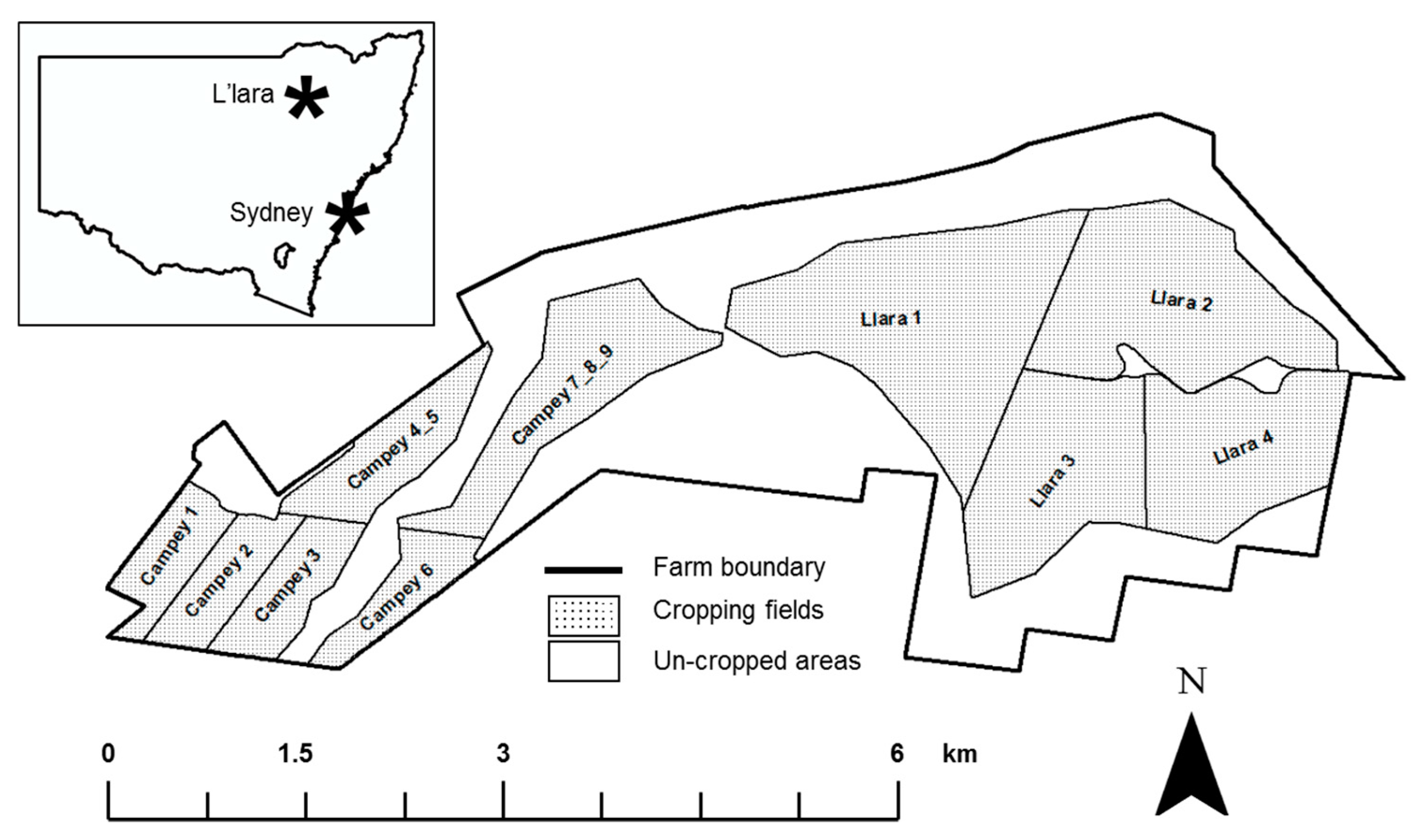
2.1. Study Site
2.2. Legacy Soil Data
2.3. Additional Soil Data
2.3.1. Data Used in Clustering Analysis
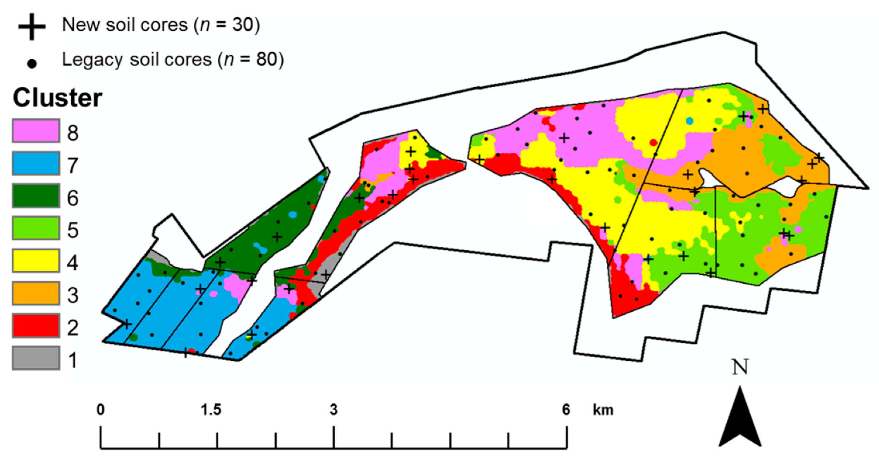
2.3.2. Clustering Analysis and Site Selection
2.3.3. Sampling Details
2.4. Vertical Depth Modelling/Resampling of Profiles
2.5. Modelling and Mapping of Soil pH
2.5.1. Data used for Modelling/Mapping Soil pH
2.5.2. Modelling/Mapping Procedure
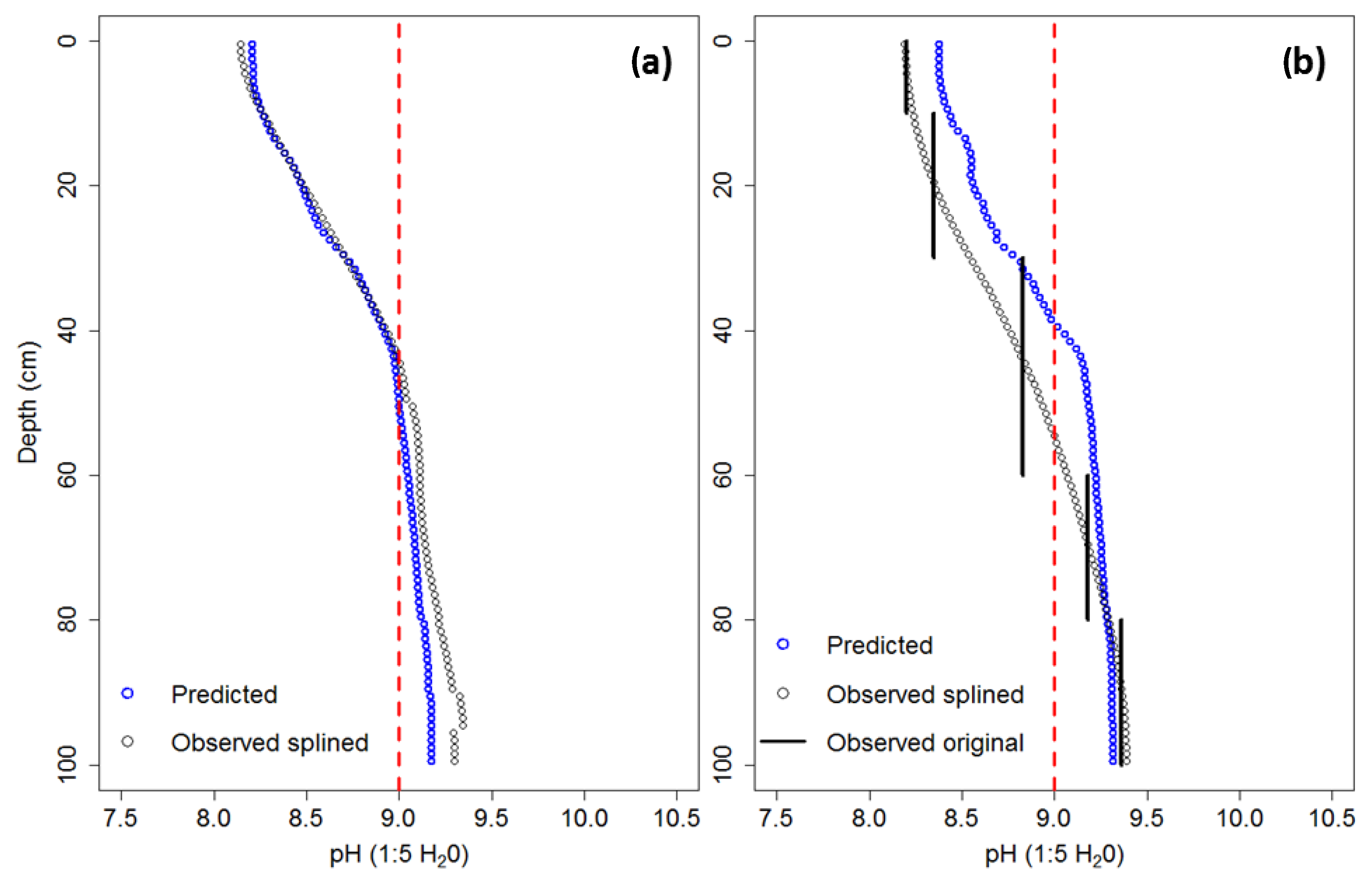
2.5.3. Model Quality and Validation
2.6. Crop Yield Data and the Relationship with Depth-to-Soil pH Constraint
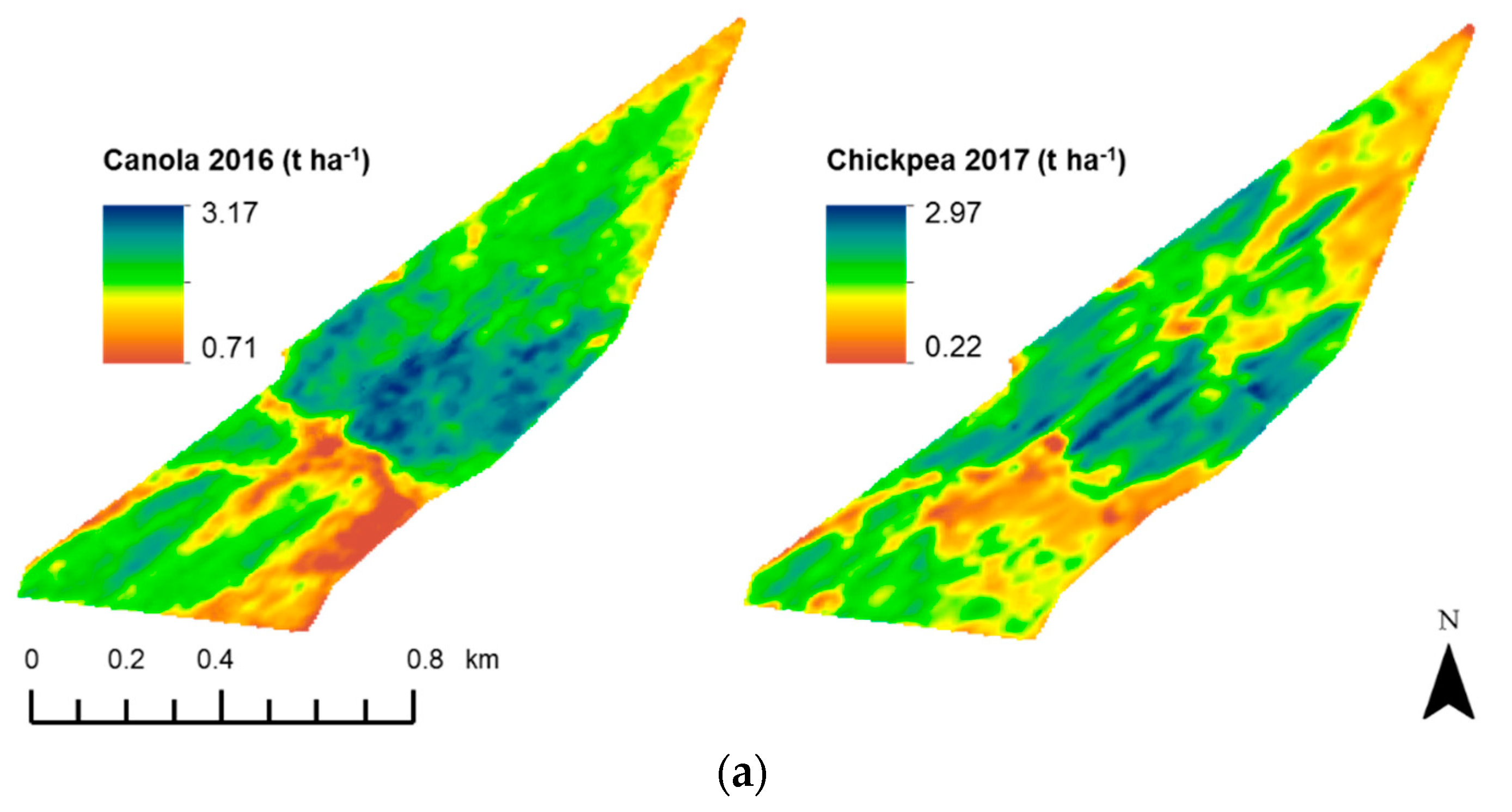
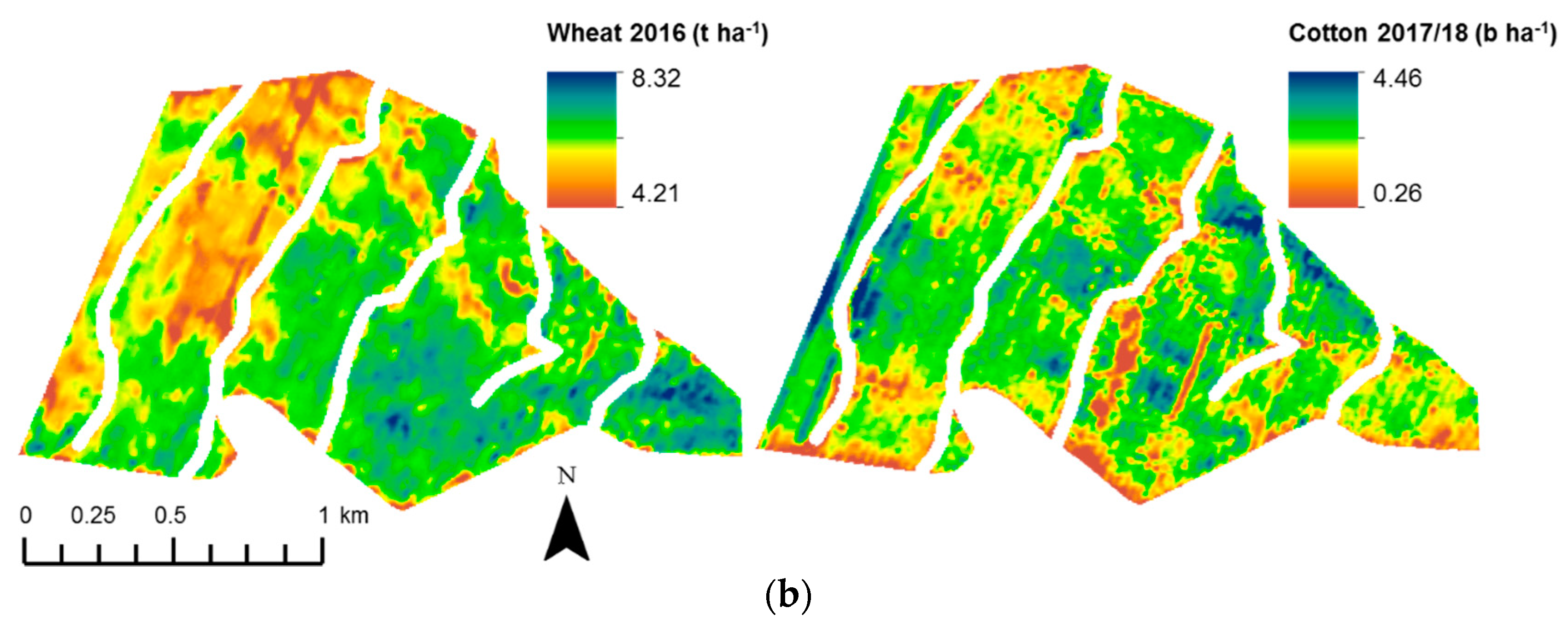
2.6.1. Crop Yield Data
2.6.2. Relationship of Crop Yield Data with Depth-to-Soil pH Constraint Data
3. Results
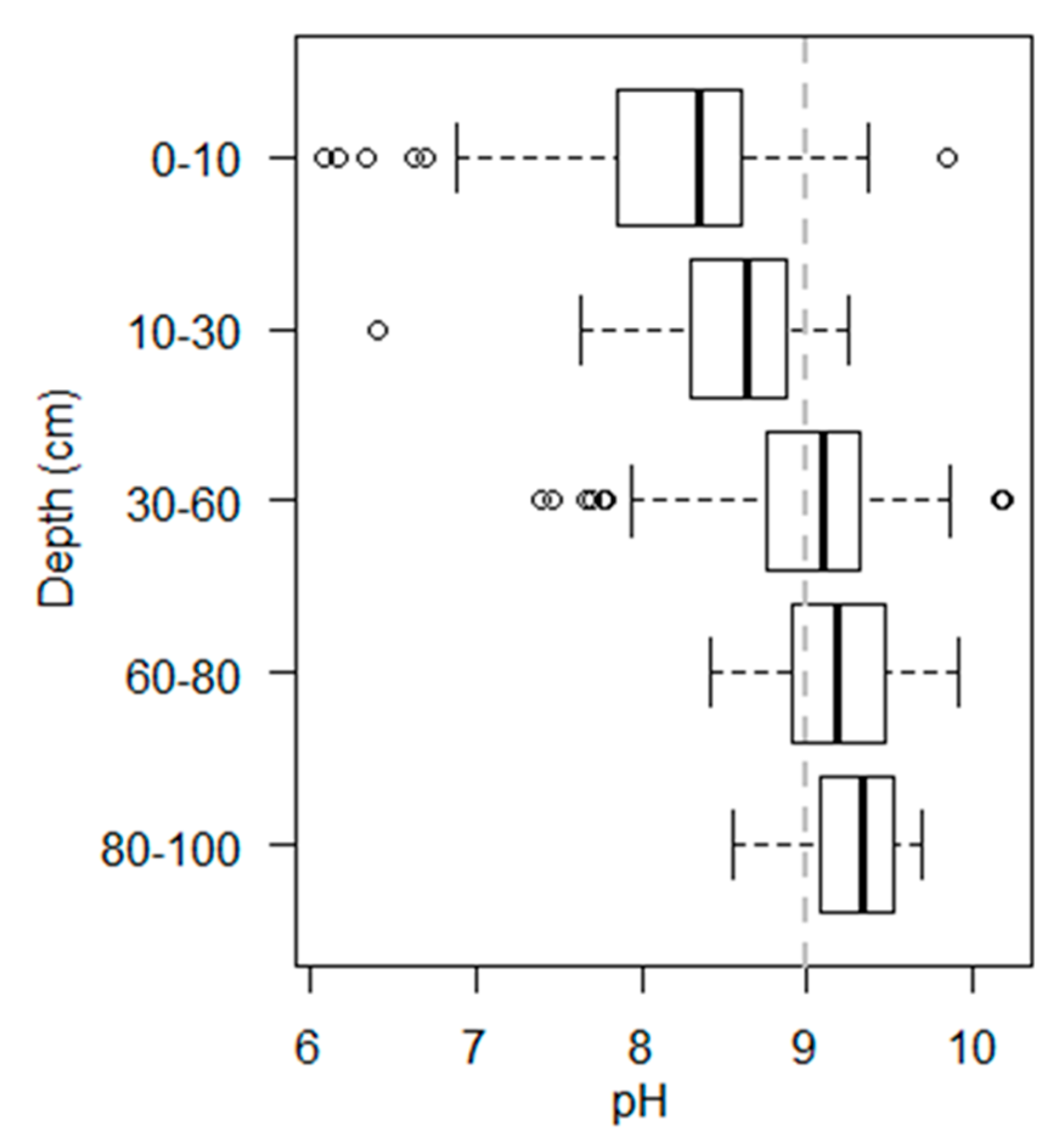
3.1. pH Variability in the Study Area
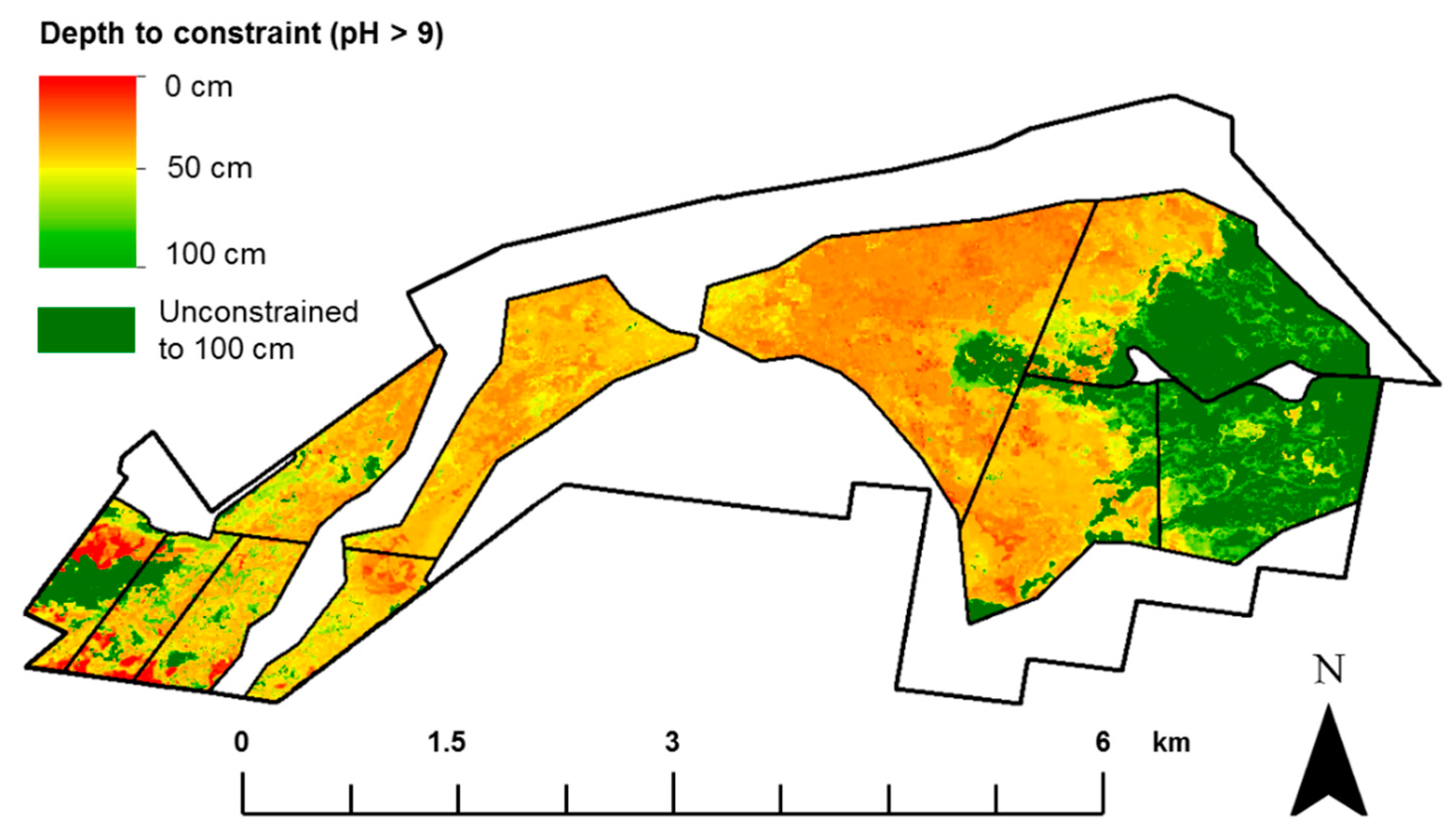
3.2. Depth-to-Soil pH Constraint
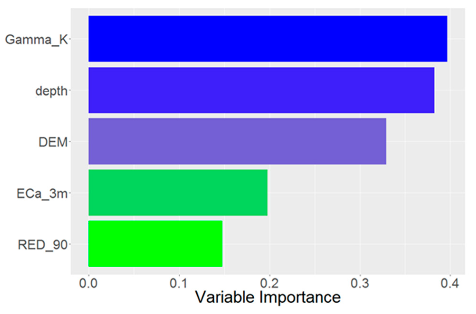
3.3. Model Quality and Variable Importance
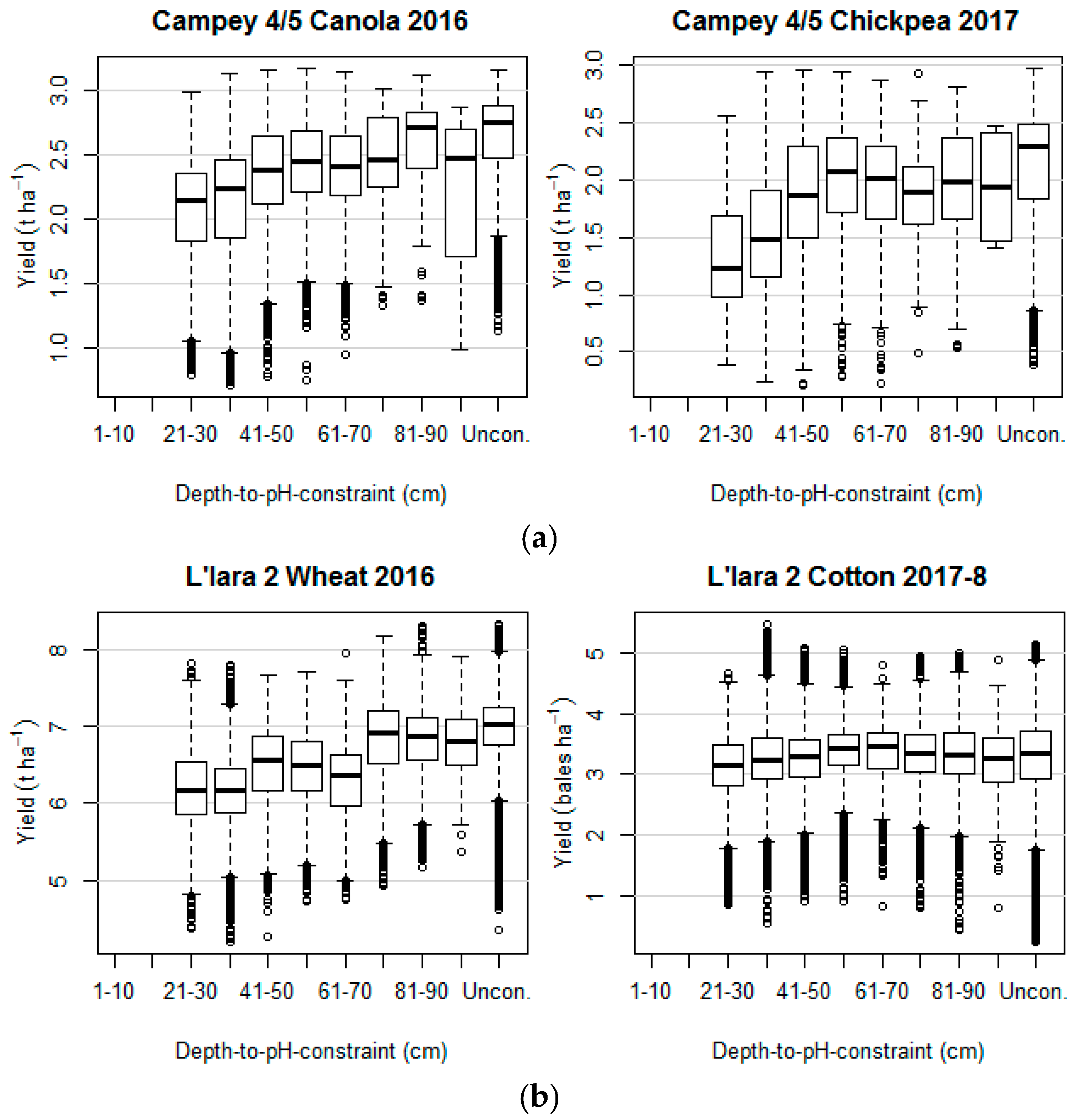
3.4. The Relationship with Crop Yield and the Depth-to-Soil pH Constraint
4. Discussion
4.1. Soil Alkalinity and Depth-to-Soil pH Constraint
4.2. Modelling/Mapping
4.2.1. Modelling/Mapping Approach and Validation
4.2.2. Predictor Variables
4.3. Relationship between Depth-to-Soil pH Constraint and Crop Yield
5. Conclusions
Author Contributions
Funding
Acknowledgments
Conflicts of Interest
References
- Dang, Y.P.; Dalal, R.C.; Routley, R.; Schwenke, G.D.; Daniells, I. Subsoil constraints to grain production in the cropping soils of the north-eastern region of Australia: An overview. Aust. J. Exp. Agric. 2006, 46, 19–35. [Google Scholar] [CrossRef]
- Odeh, I.O.A.; Todd, A.J.; Triantafilis, J.; McBratney, A.B. Status and trends of soil salinity at different scales: The case for the irrigated cotton growing region of eastern Australia. Nutr. Cycl. Agroecosyst. 1998, 50, 99–107. [Google Scholar] [CrossRef]
- Odeh, I.O.A.; Onus, A. Spatial analysis of soil salinity and soil structural stability in a semiarid region of New South Wales, Australia. Environ. Manag. 2008, 42, 265–278. [Google Scholar] [CrossRef] [PubMed]
- McKenzie, D.C.; Abbott, T.S.; Chan, K.Y.; Slavich, P.G.; Hall, D.J.M. The nature, distribution and management of sodic soils in New-South-Wales. Soil Res. 1993, 31, 839–868. [Google Scholar] [CrossRef]
- Dodd, K.; Guppy, C.; Lockwood, P.; Rochester, I. The effect of sodicity on cotton: Plant response to solutions containing high sodium concentrations. Plant Soil 2010, 330, 239–249. [Google Scholar] [CrossRef]
- McGarry, D. Soil compaction and cotton growth on a Vertisol. Soil Res. 1990, 28, 869–877. [Google Scholar] [CrossRef]
- Antille, D.L.; Bennett, J.M.; Jensen, T.A. Soil compaction and controlled traffic considerations in Australian cotton-farming systems. Crop Pasture Sci. 2016, 67, 1–28. [Google Scholar] [CrossRef]
- De Caritat, P.; Cooper, M.; Wilford, J. The pH of Australian soils: Field results from a national survey. Soil Res. 2011, 49, 173–182. [Google Scholar] [CrossRef]
- Knowles, T.A.; Singh, B. Carbon storage in cotton soils of northern New South Wales. Soil Res. 2003, 41, 889–903. [Google Scholar] [CrossRef]
- Läuchli, A.; Grattan, S.R. Soil pH extremes. Plant Stress Physiol. 2012, 194–209. [Google Scholar]
- Hazelton, P.; Murphy, M. Interpreting Soil Test Results: What Do All the Numbers Mean? CSIRO Publishing: Victoria, Australia, 2007. [Google Scholar]
- Slattery, W.J.; Conyers, M.K.; Aitken, R.L. Soil pH, aluminium, manganese and lime requirement. In Soil Analysis: An Interpretation Manual; Peverill, K.I., Sparrow, L.A., Reuter, D.J., Eds.; CSIRO: Collingwood, Australia, 1999; pp. 103–128. [Google Scholar]
- McKenzie, N.; Jacquier, D.; Isbell, R.; Brown, K. Australian Soils and Landscapes: An Illustrated Compendium; CSIRO Publishing: Clayton, Australia, 2004. [Google Scholar]
- Adamchuk, V.I.; Lund, E.D.; Reed, T.M.; Ferguson, R.B. Evaluation of an on-the-go technology for soil pH mapping. Precis. Agric. 2007, 8, 139–149. [Google Scholar] [CrossRef]
- Taylor, J.C.; Wood, G.A.; Earl, R.; Godwin, R.J. Soil factors and their influence on within-field crop variability, Part II: Spatial analysis and determination of management zones. Biosyst. Eng. 2003, 84, 441–453. [Google Scholar] [CrossRef]
- Arrouays, D.; Grundy, M.G.; Hartemink, A.E.; Hempel, J.W.; Heuvelink, G.B.M.; Hong, S.Y.; Lagacherie, P.; Lelyk, G.; McBratney, A.B.; McKenzie, N.J.; et al. Globalsoilmap: Toward a fine-resolution global grid of soil properties. Adv. Agron. 2014, 125, 93–134. [Google Scholar]
- Kirk, G.J.D.; Bellamy, P.H.; Lark, R.M. Changes in soil pH across England and Wales in response to decreased acid deposition. Glob. Chang. Biol. 2010, 16, 3111–3119. [Google Scholar] [CrossRef]
- Filippi, P.; Cattle, S.R.; Bishop, T.F.A.; Odeh, I.O.A.; Pringle, M.J. Digital soil monitoring of top- and sub-soil pH with bivariate linear mixed models. Geoderma 2018, 322, 149–162. [Google Scholar] [CrossRef]
- Bramley, R.G.V.; Ouzman, J. Farmer attitudes to the use of sensors and automation in fertilizer decision-making: Nitrogen fertilization in the Australian grains sector. Precis. Agric. 2018. [Google Scholar] [CrossRef]
- Bureau of Meteorology. Monthly climate statistics—Narrabri West Post Office (053030). Available online: http://www.bom.gov.au/climate/averages/tables/cw_053030.shtml (accessed on 18 December 2018).
- Isbell, R.F. The Australian Soil Classification; CSIRO Publishing: Melbourne, Australia, 1996. [Google Scholar]
- Boydell, B.; McBratney, A.B. Identifying potential management zones from cotton yield estimates. Precis. Agric. 2002, 3, 9–23. [Google Scholar] [CrossRef]
- Grundy, M.J.; Rossel, R.V.; Searle, R.D.; Wilson, P.L.; Chen, C.; Gregory, L.J. Soil and landscape grid of Australia. Soil Res. 2015, 53, 835–844. [Google Scholar] [CrossRef]
- Geoscience Australia. Geoscience Australia, 1 Second SRTM Digital Elevation Model (DEM). Bioregional Assessment Source Dataset. Available online: http://data.bioregionalassessments.gov.au/dataset/9a9284b6-eb45-4a13-97d0-91bf25f1187b (accessed on 4 December 2018).
- Minty, B.R.S.; Franklin, R.; Milligan, P.R.; Richardson, L.M.; Wilford, J. The radiometric map of Australia. Explor. Geophys. 2009, 40, 325–333. [Google Scholar] [CrossRef]
- Gorelick, N.; Hancher, M.; Dixon, M.; Ilyushchenko, S.; Thau, D.; Moore, R. Google Earth Engine: Planetary-scale geospatial analysis for everyone. Remote Sens. Environ. 2017, 202, 18–27. [Google Scholar] [CrossRef]
- Kodinariya, T.M.; Makwana, P.R. Review on determining number of Cluster in K-Means Clustering. Int. J. 2013, 1, 90–95. [Google Scholar]
- Bishop, T.F.A.; McBratney, A.B.; Laslett, G.M. Modelling soil attribute depth functions with equal-area quadratic smoothing splines. Geoderma 1999, 91, 27–45. [Google Scholar] [CrossRef]
- Malone, B.P.; McBratney, A.B.; Minasny, B.; Laslett, G.M. Mapping continuous depth functions of soil carbon storage and available water capacity. Geoderma 2009, 154, 138–152. [Google Scholar] [CrossRef]
- Malone, B. Ithir: Soil Data and Some Useful Associated Functions, R Package Version 1.0. 2015. Available online: https://rdrr.io/rforge/ithir/ (accessed on 20 March 2019).
- Haas, T.C. Kriging and automated variogram modelling within a moving window. Atmos. Environ. 1990, 24, 1759–1769. [Google Scholar] [CrossRef]
- Whelan, B.M.; McBratney, A.B.; Minasny, B. Vesper 1.5–Spatial Prediction Software for Precision Agriculture. In Proceedings of the 6th International Conference on Precision Agriculture, ASA/CSSA/SSSA, Madison, WI, USA, 14–17 July 2002; ASA/CSSA/SSSA: Madison, WI, USA, 2002; Volume 179. [Google Scholar]
- Department of Finance, Services and Innovation. NSW Foundation Spatial Data Framework-Elevation and Depth-Digital Elevation Model. Available online: https://data.nsw.gov.au/data/dataset/8f73f5ca-4f7f-4707-bfe2-0efbb9027107 (accessed on 4 December 2018).
- Breiman, L. Random forests. Mach. Learn. 2001, 45, 5–32. [Google Scholar] [CrossRef]
- Wright, M.N.; Ziegler, A. Ranger: A Fast Implementation of Random Forests for High Dimensional Data in C++ and R. J. Stat. Softw. 2017, 77, 1–17. [Google Scholar] [CrossRef]
- Lin, L.I.K. A concordance correlation coefficient to evaluate reproducibility. Biometrics 1989, 45, 255–268. [Google Scholar] [CrossRef]
- Orton, T.G.; Pringle, M.J.; Bishop, T.F.A. A one-step approach for modelling and mapping soil properties based on profile data sampled over varying depth intervals. Geoderma 2016, 262, 174–186. [Google Scholar] [CrossRef]
- R Core Team. R: A Language and Environment for Statistical Computing; R Foundation for Statistical Computing: Vienna, Austria, 2017. [Google Scholar]
- Taylor, J.A.; McBratney, A.B.; Whelan, B.M. Establishing Management Classes for Broadacre Agricultural Production. Agron. J. 2007, 99, 1366–1376. [Google Scholar] [CrossRef]
- Singh, B.; Odeh, I.O.A.; McBratney, A.B. Acid buffering capacity and potential acidification of cotton soils in northern New South Wales. Soil Res. 2003, 41, 875–888. [Google Scholar] [CrossRef]
- Day, A.D.; Ludeke, K.L. Soil Alkalinity. In Plant Nutrients in Desert Environments; Adaptations of Desert Organisms; Springer: Berlin/Heidelberg, Germany, 1993. [Google Scholar]
- Shafique, M.; Meijde, M.; Rossiter, D.G. Geophysical and remote sensing-based approach to model regolith thickness in a data-sparse environment. Catena 2011, 87, 11–19. [Google Scholar] [CrossRef]
- Wilford, J.R.; Thomas, M. Predicting regolith thickness in the complex weathering setting of the central Mt Lofty Ranges, South Australia. Geoderma 2013, 206, 1–13. [Google Scholar] [CrossRef]
- Wilford, J.R.; Searle, R.; Thomas, M.; Pagendam, D.; Grundy, M.J. A regolith depth map of the Australian continent. Geoderma 2016, 266, 1–13. [Google Scholar] [CrossRef]
- Blackmore, S.; Godwin, R.J.; Fountas, S. The Analysis of Spatial and Temporal Trends in Yield Map Data Over Six Years. Biosyst. Eng. 2003, 84, 455–466. [Google Scholar] [CrossRef]
- Blackmore, S. The interpretation of trends from multiple yield maps. Comput. Electron. Agric. 2000, 26, 37–51. [Google Scholar] [CrossRef]
- Guo, W. Spatial and temporal trends of irrigated cotton yield in the Southern High Plains. Agronomy 2018, 8, 298. [Google Scholar] [CrossRef]
- Shatar, T.M.; McBratney, A.B. Empirical modeling of relationships between sorghum yield and soil properties. Precis. Agric. 1999, 1, 249–276. [Google Scholar] [CrossRef]
- Schepers, A.R.; Shanahan, J.F.; Liebig, M.A.; Schepers, J.S.; Johnson, S.H.; Luchiari, A., Jr. Appropriateness of management zones for characterizing spatial variability of soil properties and irrigated corn yields across years. Agron. J. 2004, 96, 195–203. [Google Scholar] [CrossRef]
- Adeoye, G.O.; Agboola, A.A. Critical levels for soil pH, available P, K, Zn and Mn and maize ear-leaf content of P, Cu and Mn in sedimentary soils of South-Western Nigeria. Fertil. Res. 1985, 6, 65–71. [Google Scholar] [CrossRef]
- Northcote, K.H.; Skene, J.K.M. Australian Soils with Saline and Sodic Properties; CSIRO Soil Publication No. 27; CSIRO Division of Soils: Melbourne, Australia, 1972. [Google Scholar]
- Filippi, P.; Cattle, S.R.; Bishop, T.F.A.; Pringle, M.J.; Jones, E.J. Monitoring changes in soil salinity and sodicity to depth, at a decadal scale, in a semiarid irrigated region of Australia. Soil Res. 2018, 56, 696–711. [Google Scholar] [CrossRef]
- Soil Conservation Service. Soil Conservation Service. Soil Survey Division Staff Soil survey manual. In U.S. Department of Agriculture Handbook 18; US Government Printing Office: Washington, DC, USA, 1993. [Google Scholar]


| Data Type | Data Description | Resolution | |
|---|---|---|---|
| On-farm | ECa | Dual EM-21S (0–3.0 m) | 5 m |
| Gamma radiometrics | Potassium (K) | 5 m | |
| Public | Elevation | DEM | 5 m |
| Landsat 7—red band | 90th percentile (2000–2017) | 30 m |
| Depth (cm) | 0–10 | 11–20 | 21–30 | 31–40 | 41–50 | 51–60 | 61–70 | 71–80 | 81–90 | 91–100 | Unconstrained within 100 cm |
|---|---|---|---|---|---|---|---|---|---|---|---|
| Area (ha) | 11 | 16 | 183 | 339 | 128 | 51 | 23 | 32 | 37 | 4 | 245 |
| Area (%) | 1.0 | 1.5 | 17.1 | 31.7 | 12.0 | 4.8 | 2.2 | 3.0 | 3.5 | 0.3 | 23.0 |
| Validation Resolution | Lin’s Concordance Correlation Coefficient (LCCC) | Root Mean Square Error (RMSE) |
|---|---|---|
| Splined 1 cm | 0.63 | 0.47 |
| Original sampling depth | 0.66 | 0.51 |
| Campey 4/5 | L’lara 2 | |||
|---|---|---|---|---|
| Canola ‘16 | Chickpea ‘17 | Wheat ‘16 | Cotton ‘17/18 | |
| rs | 0.66 | 0.58 | 0.75 | 0.37 |
© 2019 by the authors. Licensee MDPI, Basel, Switzerland. This article is an open access article distributed under the terms and conditions of the Creative Commons Attribution (CC BY) license (http://creativecommons.org/licenses/by/4.0/).
Share and Cite
Filippi, P.; Jones, E.J.; Ginns, B.J.; Whelan, B.M.; Roth, G.W.; Bishop, T.F.A. Mapping the Depth-to-Soil pH Constraint, and the Relationship with Cotton and Grain Yield at the Within-Field Scale. Agronomy 2019, 9, 251. https://0-doi-org.brum.beds.ac.uk/10.3390/agronomy9050251
Filippi P, Jones EJ, Ginns BJ, Whelan BM, Roth GW, Bishop TFA. Mapping the Depth-to-Soil pH Constraint, and the Relationship with Cotton and Grain Yield at the Within-Field Scale. Agronomy. 2019; 9(5):251. https://0-doi-org.brum.beds.ac.uk/10.3390/agronomy9050251
Chicago/Turabian StyleFilippi, Patrick, Edward J. Jones, Bradley J. Ginns, Brett M. Whelan, Guy W. Roth, and Thomas F.A. Bishop. 2019. "Mapping the Depth-to-Soil pH Constraint, and the Relationship with Cotton and Grain Yield at the Within-Field Scale" Agronomy 9, no. 5: 251. https://0-doi-org.brum.beds.ac.uk/10.3390/agronomy9050251