Maize Kernel Abortion Recognition and Classification Using Binary Classification Machine Learning Algorithms and Deep Convolutional Neural Networks

Abstract

Maize kernel traits such as kernel length, kernel width, and kernel number determine the total kernel weight and, consequently, maize yield. Therefore, the measurement of kernel traits is important for maize breeding and the evaluation of maize yield. There are a few methods that allow the extraction of ear and kernel features through image processing. We evaluated the potential of deep convolutional neural networks and binary machine learning (ML) algorithms (logistic regression (LR), support vector machine (SVM), AdaBoost (ADB), Classification tree (CART), and the K-Neighbor (kNN)) for accurate maize kernel abortion detection and classification. The algorithms were trained using 75% of 66 total images, and the remaining 25% was used for testing their performance. Confusion matrix, classification accuracy, and precision were the major metrics in evaluating the performance of the algorithms. The SVM and LR algorithms were highly accurate and precise (100%) under all the abortion statuses, while the remaining algorithms had a performance greater than 95%. Deep convolutional neural networks were further evaluated using different activation and optimization techniques. The best performance (100% accuracy) was reached using the rectifier linear unit (ReLu) activation procedure and the Adam optimization technique. Maize ear with abortion were accurately detected by all tested algorithms with minimum training and testing time compared to ear without abortion. The findings suggest that deep convolutional neural networks can be used to detect the maize ear abortion status supplemented with the binary machine learning algorithms in maize breading programs. By using a convolution neural network (CNN) method, more data (big data) can be collected and processed for hundreds of maize ears, accelerating the phenotyping process.

1. Introduction

Maize (Zea mays L.) productivity is strongly related to the number and mass of harvested kernels which are the key grain yield determinants. The number of kernels per ear is a function of ear length (kernels per row) and kernel rows per ear [1]. In most cases, kernels at the tip of the ear cease dry matter accumulation (i.e., abort) very early in their development, and because of their greatly reduced mass, aborted kernels represent a significant grain yield loss. Kernel abortion may occur throughout the ear, not just at the tip [2]. Failure to form a kernel could occur for a variety of reasons, such as a defective ovary, pollination failure, or abortion of the fertilized ovary [3], usually caused by stressful conditions (drought, heat stress, nutritional deficiencies) [4,5].

Accurate estimation or prediction of the kernel number per ear together with the extent of kernel abortion can inform breeding for yield improvement, especially under stressful conditions [1]. There are few methods that allow the extraction of ear and kernel attributes through image processing. These methods enable to significantly reduce the cost of data collection through reliance on simple cameras and open-source image processing computational pipelines [6,7,8]. Ears are a primary agricultural product of maize, which has led the majority of previous phenotyping efforts to focus on aspects of the ear that influence yield, such as ear size, row number, and kernel dimensions [7,8,9]. Among the phenotyping methods, one was patented by Pioneer [10]. It enables to extract kernel count, kernel size distribution, proportion of aborted kernels, and other information using image processing algorithms that include, without limitation, filtering, water shedding, thresholding, edge finding, edge enhancement, color selection, and spectral filtering. Another method involves scoring maize kernel traits based on line-scan imaging and provides 12 maize kernel traits through image processing under controlled lighting conditions [9]. In 2017, Miller et al. proposed three custom algorithms designed to compute kernel features automatically from digital images acquired by a low-cost platform [8]. Shen et al. (2018) reported another method that provides kernel counts from ear photos, assuming that a maize ear has double the number of rows and kernels than can be visible on a photo [11]. These methods proved to be very useful for ear phenotyping but, except for the pioneer-patented method, they do not enable to assess the extent of kernel abortion on the ear.

In fact, kernel abortion represents a major challenge to the extraction of maize ear and kernel features through image processing. Traditional approaches such as bio-physical modeling struggle to attain high precision and accuracy in modeling and processing images with and without abortion [12]. In addition, they do not offer the possibility of processing a large volume of data. Machine learning algorithms have emerged as a robust tool that can significantly improve data collection efficiency both in terms of volume and accuracy. According to Bengio (2009), the birth of artificial intelligence brought about deep learning and machining learning algorithms that can learn from experience and predict the future [13]. Machine learning (ML) is a type of artificial intelligence (AI) that allows software applications to become more accurate at predicting outcomes without being explicitly programmed to do so [14]. It is a branch of artificial intelligence based on the idea that systems can learn from data, identify patterns, and make decisions with minimal human intervention. There are two major branches of machine learning, namely, supervised and unsupervised. A supervised learning algorithm learns from labeled training data and helps to predict outcomes for unforeseen data while unsupervised learning algorithms learn from unlabeled training data to predict the outcome. In detecting the maize cobs abortion, the supervised machine learning methods were used since the abortion and non-abortion were properly labeled.

Deep learning is a type of machine learning that trains a computer to perform human-like tasks, such as recognizing and identifying images or making predictions. Instead of organizing data to run through predefined equations, deep learning sets up basic parameters about the data and trains the computer to learn on its own by recognizing patterns using many layers of processing [15]. Deep learning has shown high performance in object detection, classification, and segmentation [16]. Convolution neural network (CNN), as the most commonly used method of deep learning, proved to be performant in some image-based phenotyping tasks [17,18]. For example, the deep learning method was used to detect plant disease [19], to count plant stalks and calculated the stalk width [20], and CNN was employed to segment rice panicles successfully based on images [21]. Convolutional neural networks (CNNs) are a class of machine learning models that can be trained to accurately detect objects in images, making them the current standard for object recognition [22].

Machine learning presents several advantages, including (i) easy identification of trends and patterns (machine learning can review large volumes of data and discover specific trends and patterns that would not be apparent to humans), (ii) automation, (iii) continuous accuracy improvement (as ML algorithms gain experience, they keep improving in accuracy and efficiency), (iv) handling multi-dimensional and multi-variety data in dynamic or uncertain environments, and (v) a wide range of applications, which makes them more robust compared to the traditional statistical procedures [23]. In addition to all the above advantages, machine learning has also limitations mostly related to the requirements for massive, inclusive/unbiased, and good quality data sets to train on, as well as time and resources needed to achieve reasonable accuracy and relevancy and high error-susceptibility.

This research sought to assess the possibility of using binary machine learning (ML) classification algorithms or deep CNNs for detecting and classifying the kernel abortion status of maize ears. Literature suggests that binary machine learning (ML) classification algorithms for decision-support and forecasting applications in maize kernel abortion analysis have not been previously evaluated. Therefore, the specific objectives of the study were (a) to evaluate the accuracy of binary classification machine learning algorithms (logistic regression (LR), support vector machine (SVM), AdaBoost (ADB), Classification tree (CART), and the K-Neighbor (kNN)) in maize kernel abortion classification and detection, (b) to assess the abortion classification and prediction capabilities of these methods, and (c) to evaluate the capability and accuracy of convolutional neural networks (CNNs) in detecting and classifying the maize kernel abortion status.

2. Materials and Methods

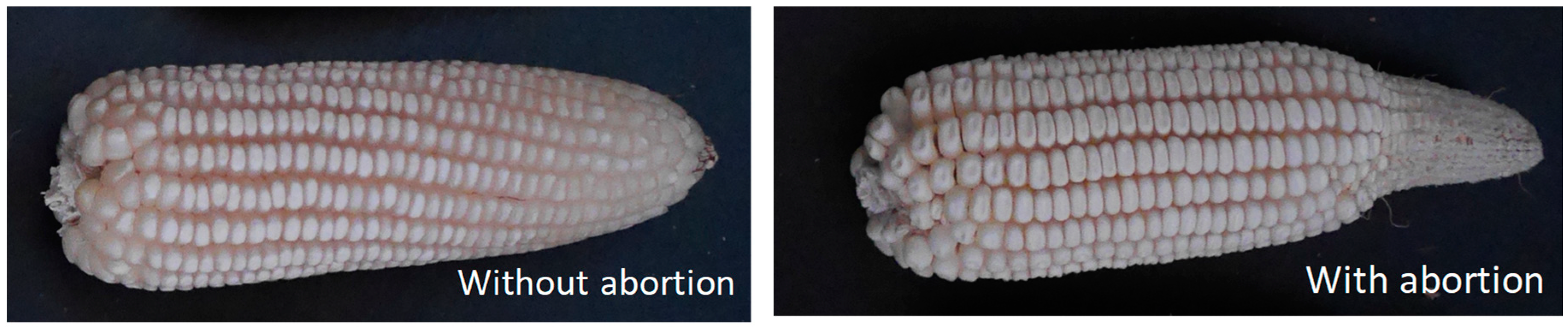
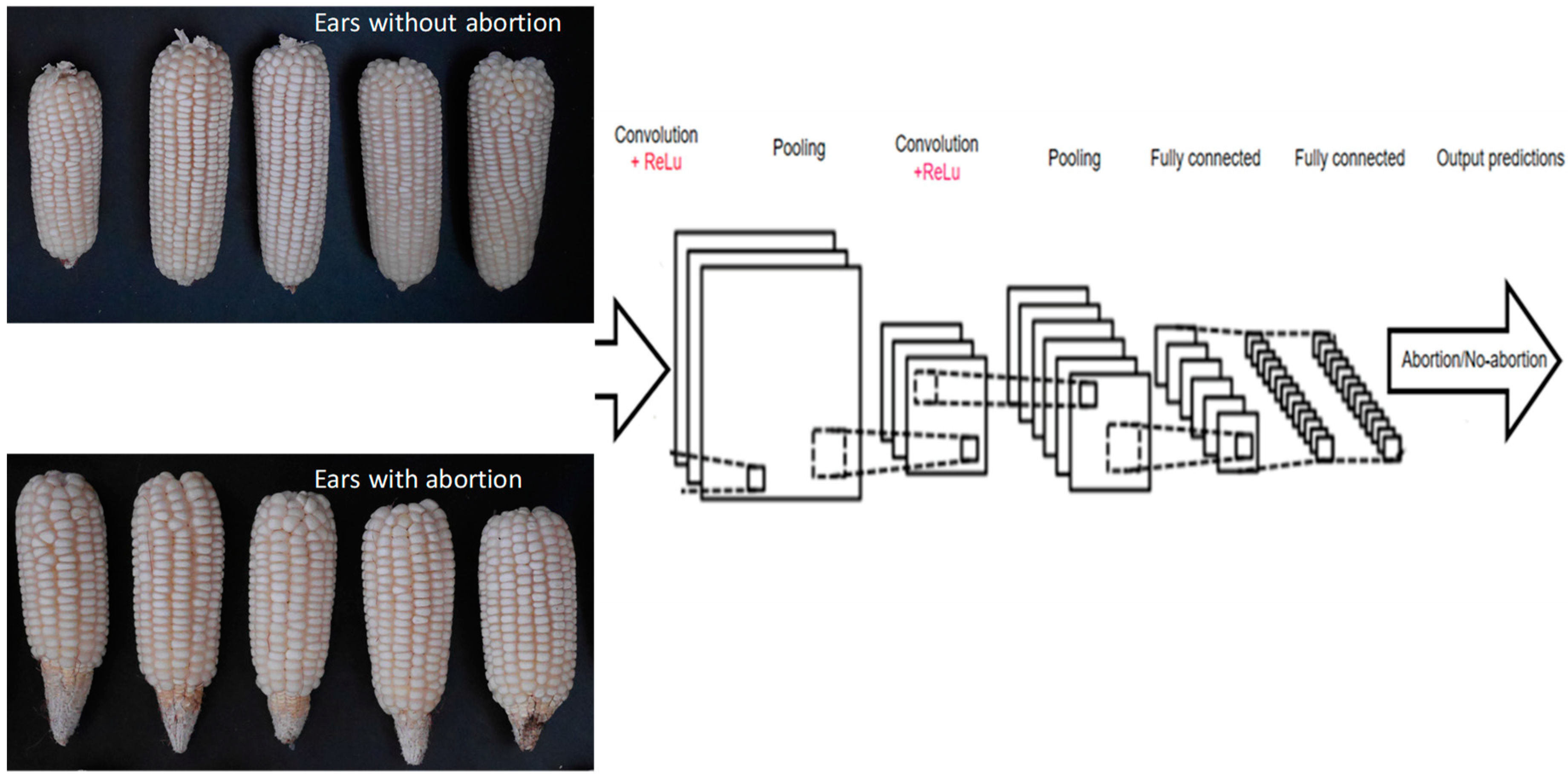
2.1. Maize Ears Photo Acquisition

Maize ears were harvested from both optimum and drought stress trials at the drought phenotyping site of the International Maize and Wheat Improvement Centre (CIMMYT) in Chiredzi, Zimbabwe (Lat, Long: −21.015432, 31.573004 (WGS 84)). A total of 60 ears were selected as a mixture of those with and without abortion and photographed individually on a black background using a 12.8 megapixels Sony camera (Cyber-shot DSC-WX220) (Figure 1).

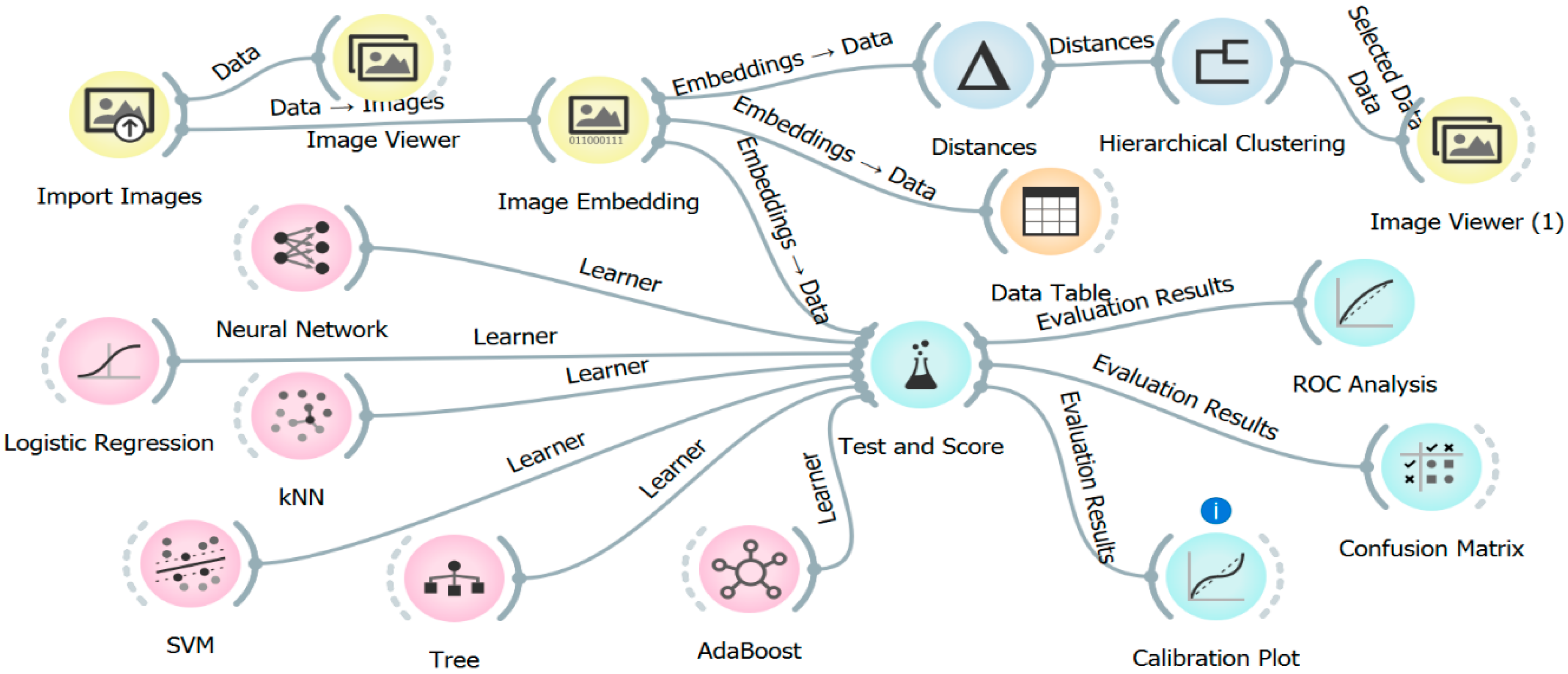
2.2. Statistical Analyses Description and Algorithms Applied

2.2.1. Image Embedding

An Image Embedding process which reads images and evaluates them locally was done in Orange using the Embedding widget as shown in Figure 2. The procedure was used as a deep learning technique for the dimensionality reduction of the input maize ear image data to be processed by general suggested binary classification machine learning algorithms and a deep convolutional neural network [24]. The process is very important for image classification as it is capable to process huge data (e.g., a 20-megapixel camera picture with 3 RGB layers means 60 million of integers as the total information stored in the image). In order to analyze maize ear images, they were converted into numeric data to enable deep and machine learning algorithms to be trained and tested. Embedding transforms raw images into a vector representation or multi-dimensional feature space (image descriptors) which contains more information than image name, width, size, and height [25]. Since the images were evaluated locally from a computer, the SqueezeNet embedder was used as it offers fast evaluation which does not require an internet connection. SqueezeNet is a deep model for image recognition that achieves AlexNet-level accuracy on ImageNet with 50x fewer parameters.

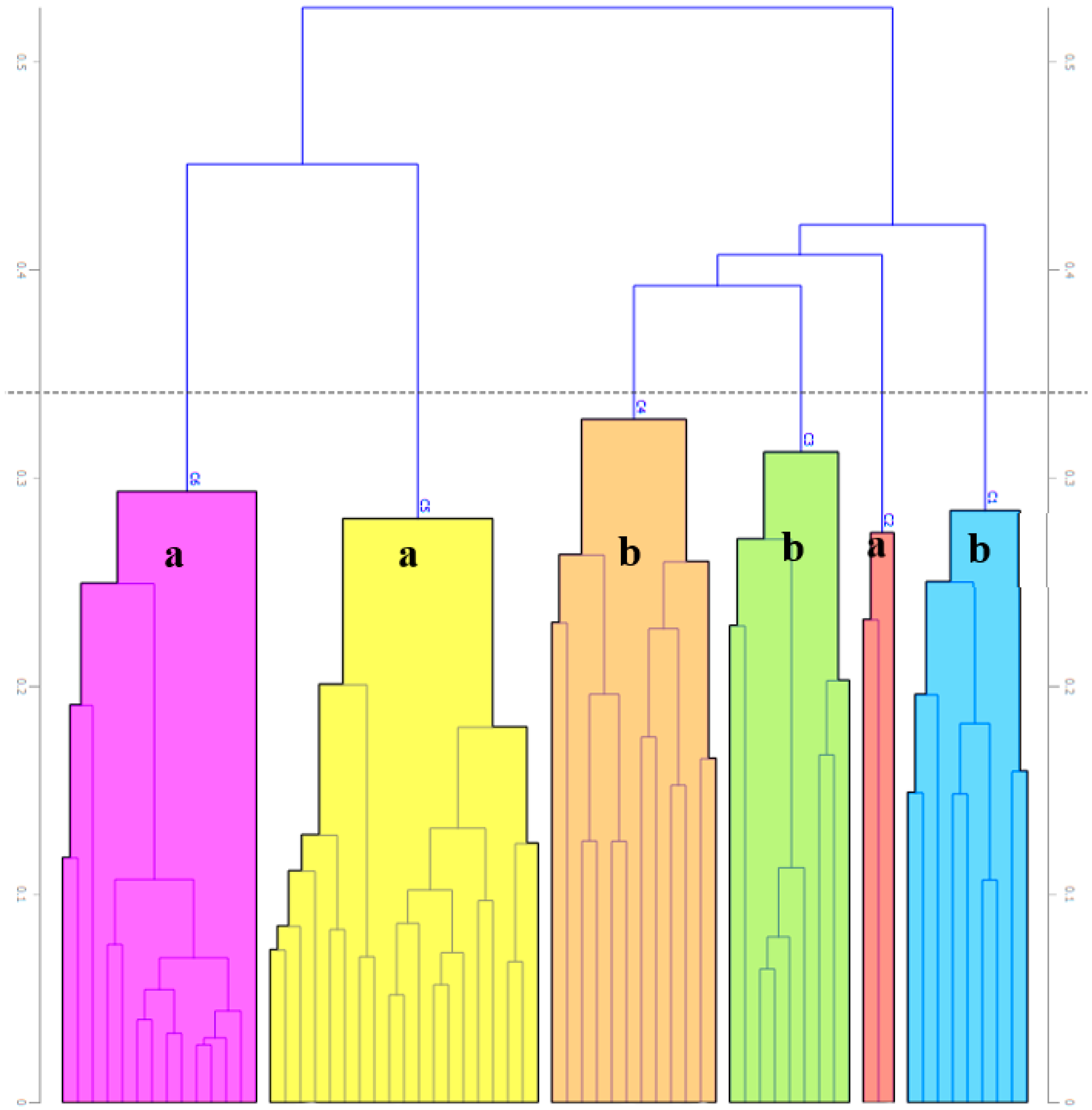
2.2.2. Image Clustering

Maize ear images comprised of two samples representing abortion and no abortion. The samples were considered as clusters to be examined using a hierarchical clustering algorithm before implementing machine learning and deep learning techniques. This enables the evaluation of the validity of the two important features differentiating the two samples, that is, images with abortion and images without abortion. Hierarchical clustering is a cluster tree (a dendrogram) that represents data, where each group (or “node”) links to two or more successor groups [26]. The groups are nested and organized as a tree, which ideally ends up as a meaningful classification scheme. Each node in the cluster tree contains a group of similar data. Nodes group on the graph next to other similar nodes. Clusters at one level join with clusters in the next level up, using a degree of similarity. The process carries on until all nodes are in the tree, which gives a visual snapshot of the data contained in the whole set. The total number of clusters is not predetermined before the start of tree creation.

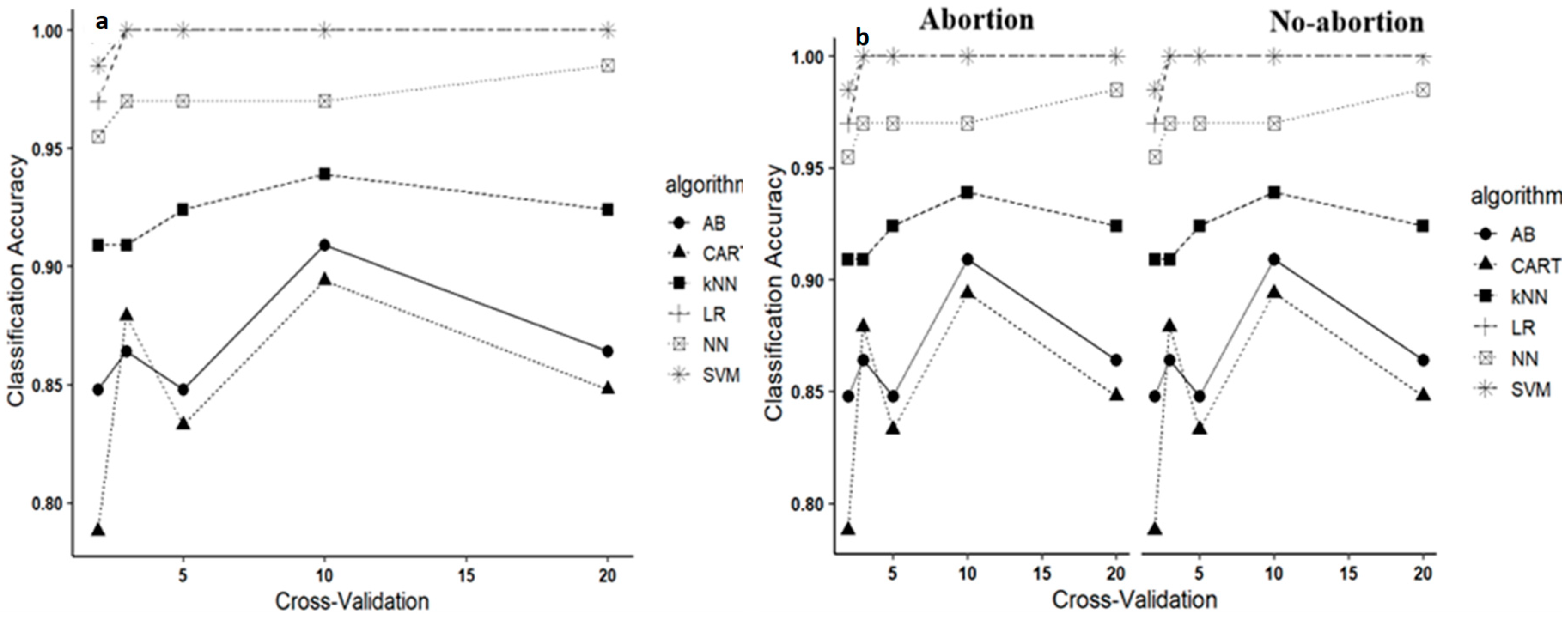
2.2.3. Training, Testing, and 10-Fold Cross-Validation

The study and construction of algorithms that can learn from and make predictions on data is the major task of deep learning and machine learning. The algorithms work by making data-driven predictions or decisions through building a mathematical model from input data [27]. A training dataset is a dataset of examples used for learning or training, that is, to fit the parameters (weights) of a classifier, and a test dataset is independent of the training dataset but follows the same probability distribution as the training dataset. In this study, 70% of the maize ear image dataset was used to train the algorithms and the remaining 30% was used as a test set. It is necessary to have a validation dataset in addition to the training and test datasets to avoid overfitting [28]. The algorithms were given a set of known images with and without abortion on which training was run (training the dataset) and a dataset of unknown data (or first seen data) against which the algorithms were tested (the validation dataset or testing set). The major use of cross-validation in this study was to test the algorithms’ abilities to classify maize ear images based on abortion status in order to flag problems such as overfitting or selection bias [29]. The 10-fold cross-validation was used, which portioned the original sample into 10 subsamples of equal size. Of the 10 subsamples, a single subsample was retained as the validation data for testing the algorithms, and the remaining 9 subsamples were used as training data.

2.3. Binary Classification Machine Learning Algorithms

General machine learning algorithms are not usually recommended for image processing and analysis especially when the classification problem is not binary (more than two classes) [30]. There are some machine learning algorithms that were examined and proved to perform very well given a binary classification problem [29]. Since the task was to classify the maize ears according to whether they have abortion or not, the following machine learning algorithms were used: logistic regression (LR), neural network (NN), support vector machine (SVM), AdaBoost (ADB), Classification tree (CART), and the K-Neighbor (kNN). Figure 2 shows how the machine learning (ML) widgets were connected in Anaconda Orange 3.24 supported by Python version 3. The images were imported using the image viewer and connected the embedding widgets which converted the images to numeric data before apportioning into training and testing datasets at the test and score widget. All the experimented algorithms were then connected to the test and score widgets for performance evaluation using receiver operating characteristic (ROC) analysis, confusion matrix, and calibration plot.

2.4. Convolutional Neural Networks

Deep learning convolutional neural networks use a similar concept as that of multilayer perceptions (Figure 3) which are made up of the input layer, hidden layer, and output layer [15]. The input layer (in(t)) consists of the imbedded multidirectional maize ear features (x₁, x₂, x₃,… x_n). It is then connected to the hidden layer (w_o(t)) where w₁, w₂, w₃, … w_n are the estimated coefficients. The number of hidden layers (neurons) can be adjusted in a general neural network to improve accuracy. This original neural network (NN) is used mainly for character recognition tasks.

Deep learning convolutional neural networks seek to exploit the unknown structure in the input distribution in order to discover good representations, often at multiple levels, with higher-level learned features defined in terms of lower-level features [30]. The convolutional neural network in Figure 4 is similar in architecture to the original neural network and classifies an input image into two categories: maize ears with and without abortion. As observed from Figure 4, on receiving a maize ear without abortion image as input, the network correctly assigns the highest probability for maize ear without abortion among the other category without abortion. The sum of all probabilities in the output layer should be one.

There are four main operations in the convolutional neural network (ConvNet) shown in Figure 4 above: convolution, non-linearity (rectifier linear unit (ReLU), pooling or subsampling, and classification fully connected layer). These operations are the basic building blocks of every convolutional neural network. Pooling (also called subsampling or down sampling) reduces the dimensionality of each feature map but retains the most important information [25]. Spatial pooling can be of different types: max, average, sum, etc. In particular, pooling

• Makes the input representations (feature dimension) smaller and more manageable;
• Reduces the number of parameters and computations in the network, therefore, controlling overfitting;
• Makes the network invariant to small transformations, distortions, and translations in the input image;
• Helps to arrive at an almost scale invariant representation of the image. This is very powerful since we can detect objects in an image no matter where they are located.

The fully connected layer is a traditional multi-layer perceptron that uses a softmax activation function in the output layer. The term “fully connected” implies that every neuron in the previous layer is connected to every neuron on the next layer. The full analysis of the deep learning convolutional neural network was conducted in Python 3 using the Keras Tensoflow library for deep learning.

2.5. Algorithms Evaluation Techniques

The performance of the tested algorithms in accurately classifying the maize ears with and without abortion was examined using different evaluation techniques, namely: confusion matrix, ROC analysis, and calibration plot.

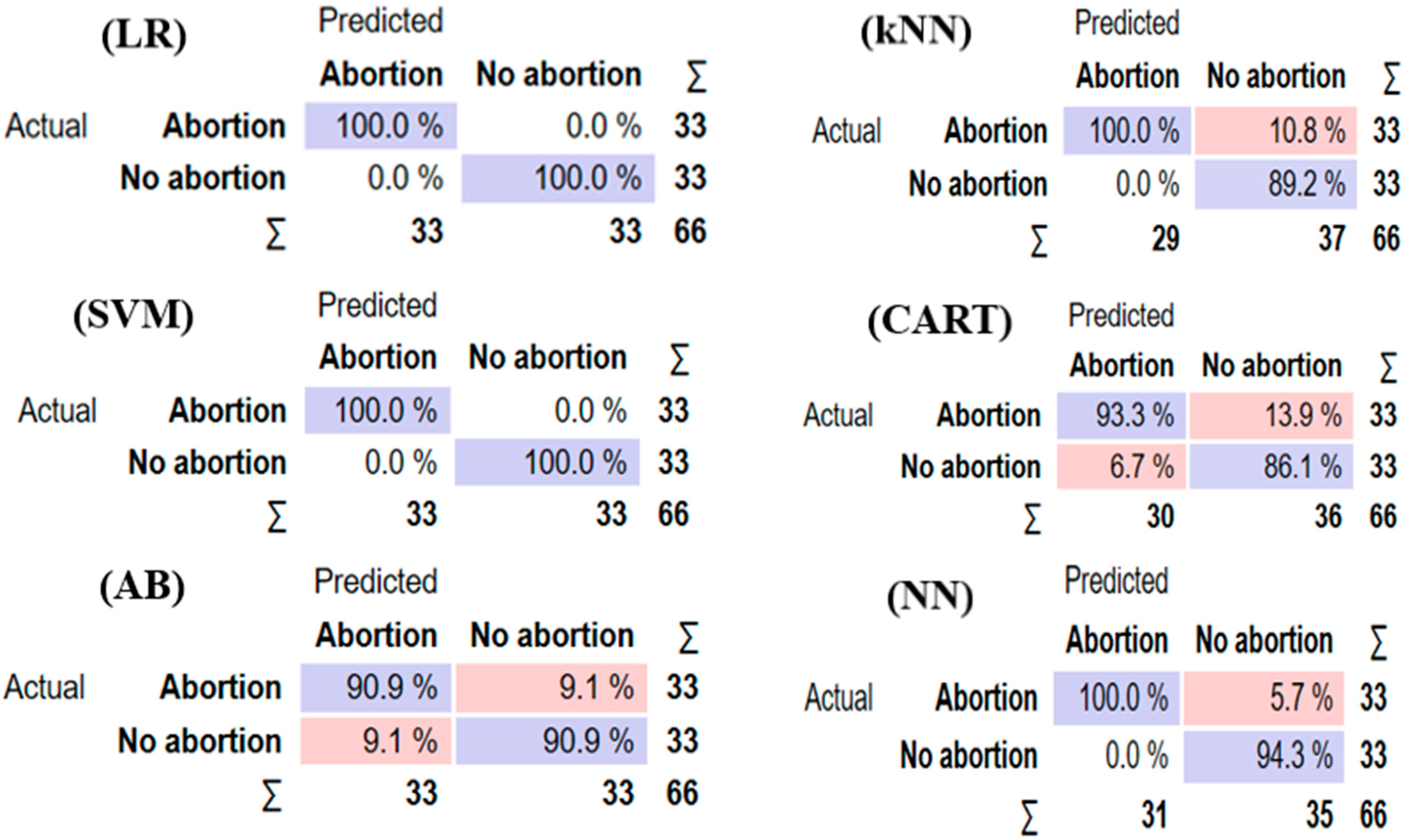
2.5.1. Confusion Matrix

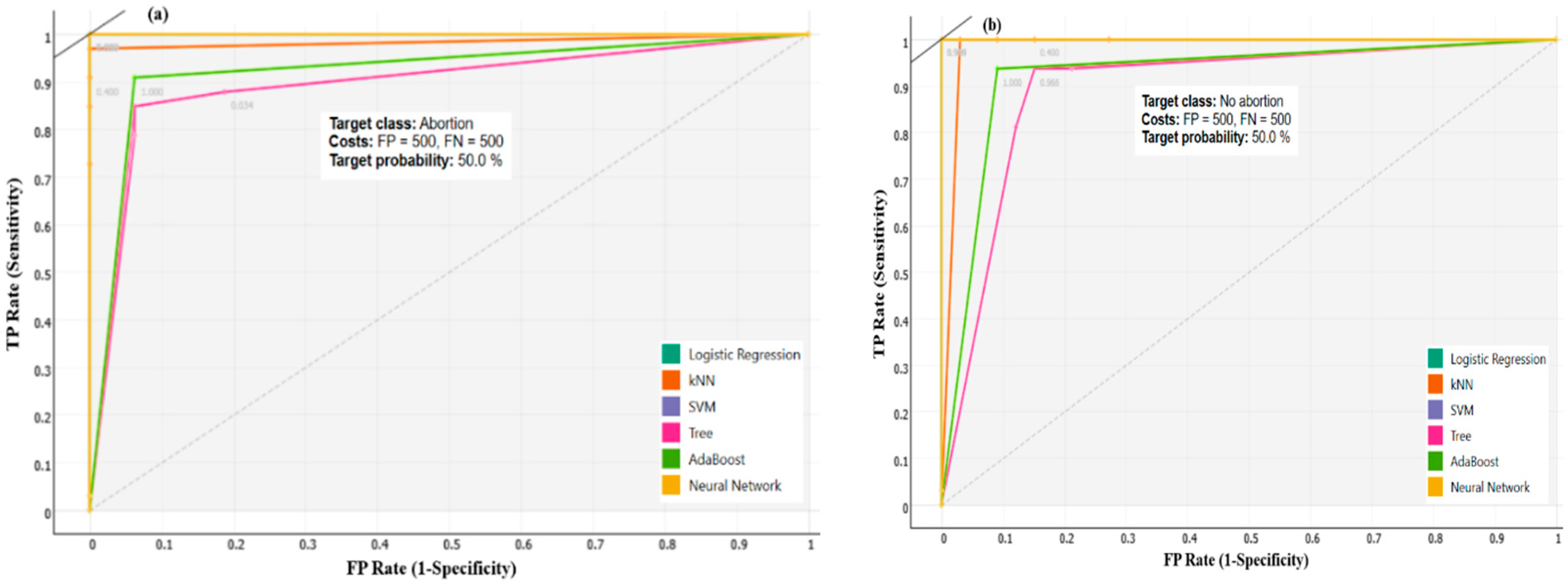
A confusion matrix is a figure or a table that was used to describe the performance of a classifier [31]. It was extracted from a test dataset for which the ground truth was known. Each class was compared with every other class and investigated how many samples were misclassified. The image detection was considered as a binary classification case with the output 0 (no abortion) and 1 (abortion). The confusion matrix contains the following major information: true positives (TP), true negatives (TN), false positives (FP/Type I error), and false negatives (FN/type II error). Accuracy matrices of all the examined algorithms were calculated from the confusion matrix as follows:

$$\mathrm{Accuracy}=\frac{TP+FP}{TP+FP+TN+FN},$$

(1)

$$\mathrm{Sensitivity}=\frac{TP}{TP+FN},$$

(2)

$$\mathrm{Specificity}=\frac{TN}{TN+FP},$$

(3)

$$\mathrm{Precision}=\frac{TP}{TP+FP},$$

(4)

$$\mathrm{Recall}=\frac{TP}{TP+FN}.$$

(5)

2.5.2. ROC Analysis

The receiver operating characteristic (ROC) analysis was a useful way to assess the accuracy of model predictions by plotting sensitivity versus 1-specificity of a classification test (as the threshold varies over an entire range of diagnostic test results) [31]. The full area under a given ROC curve or area under the curve (AUC) formulates an important statistic that represents the probability that the prediction will be in the correct order when a test variable is observed. The ROC analysis supports the inference regarding a single AUC, precision-recall (PR) curves, and provides options for comparing two ROC curves that are generated from either independent groups or paired subjects.

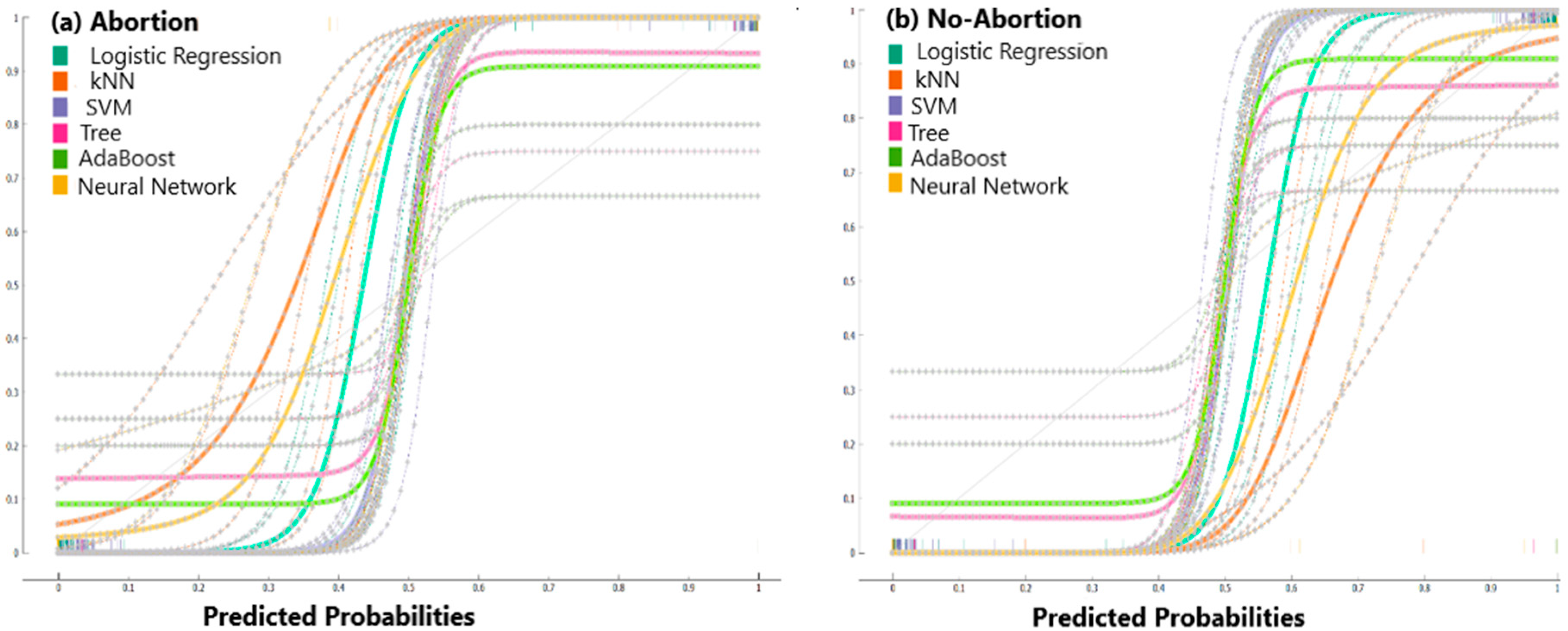
2.5.3. Calibration Plot

The calibration plot was used to assess the goodness of fit of the algorithms graphically. It enables to qualitatively compare an algorithm’s predicted probability of an event to the empirical probability. Assessing calibration by plotting a scatter plot smoother and overlaying a diagonal line represents the line of perfect calibration. If the smoother lies close to the diagonal, the algorithm is well calibrated [25]. If there is a systematic deviation from the diagonal line, it indicates that the algorithm might be misspecified.

3. Results and Discussion

3.1. Binary Classification Algorithms

Maize ears encode a vast amount of information in agriculture and provide insights into the value of a crop through yield and seed quality [32]. The maize cobs with their abortion status were subjected to clustering analysis using the hierarchical algorithm. The results were presented in form of a dendrogram (Figure 5). Distances between rows were calculated using the cosine metric and ward linkage. The images were clustered from top to down or using divisive clustering. The dendrogram shows six major computed clusters and each represents a single group of images. A cluster labeled (a) represents images without abortion and (b) images with abortion. The hierarchical clustering algorithm accurately identified the abortion status of all the images as the clusters contain maize cobs images with the same similarity. Abortion was easily detected and recognized which makes it possible to apply the binary classification ML algorithms and deep convolutional neural networks. The results of the hierarchical clustering algorithm are in agreement with the findings in other researches where they were used to recognize and discriminate maize and weed species with 100% accuracy [33]. The approach was also successfully evaluated in more complicated clustering problems such as in radiomic machine learning classifiers for prognostic biomarkers of advanced nasopharyngeal carcinoma [34]. Clustering brings an important aspect to the classification aspect but the two are different. Class labels of images were not given during clustering and the learning process was unsupervised as the hierarchical algorithms manages to identify the class labels on its own. In classification, the class labels are given and the learning process is supervised. All the experimented algorithms in the study were supervised machine learning algorithms that were trained based on the two major identified clusters of the images with and without abortion.

After clustering analysis, the six tested binary ML classification algorithms were trained and their performance evaluated on a test dataset based on a 10-fold cross-validation. The evaluation criteria included the time in seconds taken by each algorithm during training and testing, the classification accuracy (CA), precision, recall, logarithmic loss (LogLoss), and specificity. The minimum time in seconds was taken by the CART algorithm during training and testing (1.55 and 0.00 s, respectively). kNN, ADB, and LR took an average of 2 s during training and testing. Neural network (NN) and the SVM algorithms took the maximum time in seconds: an average of 9 s during training and 3 s during testing. All the algorithms performed very well as their classification accuracies were greater than 85% (

Table 1. The evaluation metrics of all the tested binary classification algorithms derived from the confusion matrix. Logistic regression (LR), neural network (NN), support vector machine (SVM), AdaBoost (ADB), Classification tree (CART), and the K-Neighbor (kNN).

Algorithm	Train Time (s)	Test Time (s)	CA	F1	Precision	Recall	LogLoss	Specificity
CART	1.550	0.000	0.894	0.894	0.897	0.894	3.194	0.894
AB	3.245	1.502	0.909	0.909	0.909	0.909	3.140	0.909
kNN	2.572	2.409	0.939	0.939	0.946	0.939	0.607	0.939
NN	11.683	4.186	0.970	0.970	0.971	0.970	0.060	0.970
LR	2.821	2.306	1.000	1.000	1.000	1.000	0.026	1.000
SVM	8.997	2.932	1.000	1.000	1.000	1.000	0.034	1.000

). The LR and SVM algorithms were more accurate as they reached 100% accuracy capacity. This was also supported by the corresponding precision, recall, and specificity metrics. Logarithmic loss (LogLoss) related to cross-entropy was used with the goal to minimize the prediction probability between 0 and 1. The LR and SVM algorithms were effective in minimizing the probability with values approximately equal to zero. CART and ADB failed to minimize the prediction probability with values exceeding 3, while the kNN and NN were on average with values approximately equal to one also. This implies that all the tested algorithms were effective and efficient in detecting the abortion status and classifying it according to abortion or no abortion. However, based on the 10-fold cross-validation, the best algorithms were LR and SVM while the remaining algorithms performed very well. In several other researches where the SVM was used to solve a binary image classification problem, the algorithm gave excellent precision and accuracy. In Binch et al.’s (2017) research titled ‘controlled comparison of machine vision algorithms for Rumex and Urtica detection in grassland’, the SVM gave 97.9% accuracy compared to other experimented tools [33]. In detection and classification of common types of botanical and non-botanical foreign matter that are embedded inside the cotton lint, the LR and SVM recorded 96% accuracy and precision [35]. Furthermore, the tools were also evaluated in the classification of parasites and automatic detection of thrips in strawberry crop giving approximately 100% accuracy [36]. Similar prediction power of the tested algorithms suggested the need to verify the accuracy stability as the cross-validation increased. Furthermore, given a binary image classification problem, the algorithms can be recommended as they managed to reach a favorable accuracy.

The efficiency and prediction power of the tested algorithms were also evaluated by tracing the predicted probabilities versus the calibration curve which is effective in binary response prediction and classification (Figure 6). This added value in assessing the goodness of fit of the tested algorithms. The loess smoother lies close to the diagonal line, which indicated that the tested algorithms were a good fit for the image classification data and, therefore, they can be recommended for detecting and classifying abortion in maize cobs. The loess curve is systematically close to the diagonal line for very small and very large values of the predicted probability. This indicated that the empirical probability (the proportion of events) was not higher than predicted on these intervals. In contrast, when the predicted probability is in the range (0.1, 0.45), the empirical probability is lower than predicted and this implies a lack of goodness of fit [37]. The calibration plots of the predicted abortion and no-abortion images crossed the loess line between the 0.4 and 0.5 threshold probabilities and exponentially increased to 0.9 and remained constant. Overfitting is one of the threats to ML algorithms which need to be investigated. Based on the calibration plot, the tested binary classification algorithms fitted very well.

In addition to the goodness of fit assessment, the tested algorithms’ predictions and classifications were also evaluated using the receiver operating characteristic (Figure 7). ROC analysis evaluated the sensitivity (true positive rate) of the algorithms versus the false positive rate (1-specificity). True positives denote accurate classification prediction while the false positives were regarded as correct prediction but in actual fact, they were not correct. The ROC curve shows the trade-off between sensitivity (true positive rate (TPR)) and specificity (1—false positive rate (FPR)). Classifiers that give curves closer to the top left corner indicate a better performance. The ROC curves exhibited a sharp bend which is an indication of perfect performance in classification. As the true positive suggests how good the algorithm is in detecting a target class, all the tested binary classification algorithm curves were very close to the top left corner, which indicated the best performance [37]. Across all the abortion statuses, the algorithms performed very well with all curves close to the top left corner that is the true positive rate.

The confusion matrix summarizes the performance of all the algorithms as the major metrics can also be derived from it. Figure 8 shows the actual and predicted prediction and classification proportions of the two classes (abortion and no abortion). The LR and SVM algorithms accurately predicted and classified the abortion status of the maize cobs as they gave 100% correct prediction and 0% misclassifications. The kNN correctly predicted abortions with an accuracy of 100% while misclassified no abortion with only 10.8%. This indicated that the algorithm can be used to solve the classification problem with a very low misclassification error. The CART algorithm also gave a very low misclassification rate of 13% under no abortion and 6.7 under abortion, which indicated that the algorithm performed very well. AdaBoost gave a similar misclassification rate (9.1%) under all the abortion statuses and the classification accuracy was approximately 91%. The NN was 100% accurate under abortion without any misclassification and 94.3% under no-abortion images with only 5.7% misclassification (meaning, images which were identified as if they had no abortion but in fact they had). The confusion matrix becomes the major algorithms evaluation technique as it gives a clear comparison of the predicted and the actual images. Results of the confusion matrix also indicated that the SVM and LR algorthms are the best perfomers as they did not have any misclassification error. A similar trend of performance was also discovered when the tools were evaluated for an active learning system for weed species recognition based on hyperspectral sensing [38]. However, all the other tested binary classification ML algorithms had very low misclassification errors. In the study, a balanced number of pictures were used, each class represented by 33 images, which makes the comparison and evaluation of the tested tools fair.

Accuracy reliability and validity is also important when evaluating the performance of algorithms (Figure 9). This was achieved by investigating the classification accuracy at different cross-validation sizes (2, 3, 5, 20, and 20). The cross-validation size increases the classification accuracy of LR and SVM remaining constant at 1 (100%). This gives evidence of consistency and accuracy of the tools as the number of training subsamples increases or decreases. The NN showed a significant increase as the cross-validation reached 20. The remaining tested algorithms’ classification accuracy fluctuated between 0.80 and 0.90 which implies that they were not stable in giving the expected accuracy. The evaluation was based on the general comparison and abortion status. The best performers maintained the same trend under abortion and no abortion which indicated consistency in their prediction power. Some algorithms are quick to reach the best accuracy at a single cross-validation size and fail to maintain or increase the performance. This is evidence of inconsistencies and, therefore, the recommendation must be based on the algorithms that exponentially increase in accuracy or remain constant when the cross-validation is adjusted [39].

3.2. Deep Convolutional Neural Network

Unlike other machine learning techniques, the deep convolutional network comes with different activation and optimization techniques to boost performance (

Table 2. Deep convolutional neural network results based on the 10-fold cross-validation and 100 neurons, using different activation and optimization techniques. AUC = area under the curve, CA = classification accuracy, LogLoss = logarithmic loss, SGD = stochastic gradient descent, L-BFGS-B = limited-memory BFGS (L-BFGS or LM-BFGS), Logistic = logistic activation function, ReLu = rectifier linear unit, Tanh = hyperbolic tangent activation function, and Identity = identity activation function.

Activation	Solver	AUC	CA	F1	Precision	Recall	LogLoss	Specificity
Identity	Adam	1.000	1.000	1.000	1.000	1.000	0.015	1.000
	L-BFGS-B	1.000	0.985	0.985	0.985	0.985	0.041	0.985
	SGD	1.000	0.970	0.970	0.971	0.970	0.040	0.970
Logistic	Adam	1.000	1.000	1.000	1.000	1.000	0.014	1.000
	L-BFGS-B	1.000	0.985	0.985	0.985	0.985	0.027	0.985
	SGD	1.000	0.985	0.985	0.985	0.985	0.027	0.985
Tanh	Adam	1.000	1.000	1.000	1.000	1.000	0.014	1.000
	L-BFGS-B	1.000	0.985	0.985	0.985	0.985	0.041	0.985
	SGD	1.000	0.985	0.985	0.985	0.985	0.023	0.985
ReLu	Adam	1.000	1.000	1.000	1.000	1.000	0.014	1.000
	L-BFGS-B	1.000	0.985	0.985	0.985	0.985	0.041	0.985
	SGD	1.000	0.985	0.985	0.985	0.985	0.023	0.985

). In evaluating deep convolutional neural network algorithm, four activation functions (Logistic, Identity, hyperbolic tangent activation function (Tanh), and ReLu) and three optimization techniques (Adam, SGD, and L-BFGS-B) were used. Across all the activation and optimization techniques, the area under the curve (AUC) was equal to one, implying that the deep neural network performed very well, as there was a 100% chance of its ability to distinguish the abortion status. Classification accuracy (AC) using the Adam optimization technique was 1 (100%) across all the used activation methods. Stochastic gradient descent (SDG) and L-BFGS-B = Limited-memory BFGS (L-BFGS or LM-BFGS) classification accuracy was approximately 100% across all activation methods. The other metrics such as precision, f1 score, Recall, and specificity of the deep convolutional neural network followed the same trend to their corresponding classification accuracy. LogLoss minimizes the prediction probability between 0 and 1. The Adam optimization technique minimizes the LogLoss to zero at different examined activation techniques, while the other optimization techniques were also giving LogLoss reduction. Designed specifically for image recognition, the deep neural network accurately predicted and classified the image abortion status. The stability and consistency were examined using different optimization and activation techniques. Adam and ReLu gave the best accuracy. The CNN method is more popular in various non-agriculture fields, but its application in the agricultural research has been witnessed. In 2005, the approach was successfully used in the detection of yellow rust-infected and healthy winter wheat under field circumstances from data fusion of hyper-spectral reflection and multi-spectral fluorescence imaging giving an accuracy of 99.4% [40]. CNN was further used in wheat research to identify and discriminate yellow rust-infected, nitrogen-stressed, and healthy winter wheat in field conditions, and the approach gave 99.92% accuracy [41]. In addition to wheat-related studies, the CNN method was suggested to be the best method with 99.53% accuracy in the detection of plant diseases [19]. In legumes, the approach was used in the identification and classification of three legume species: soybean, as well as white and red bean, giving an accuracy of 98.8% [42]. According to the ML in agriculture review paper, artificial and deep neural networks were successfully used in the following fields: yield prediction, disease detection, weed detection crop quality, species recognition, animal welfare, livestock production, water management, and soil management [33]. The findings of this study recommend the application and use of deep convolutional neural networks (CNNs) supplemented with binary classification ML algorithms in detecting and classifying the maize cobs images abortion status.

4. Conclusions

The hierarchical clustering algorithm precisely detected the two abortion clusters (with and without abortion) from the maize ears images without being supervised and suggested the possibility of using binary machine learning algorithms and a deep convolutional neural network in maize ear phenotyping. All the tested binary machine learning algorithms performed well in detecting and classifying abortion, but the SVM and LR were far better than the other tested methods. In evaluating the used methods at different cross-validation intervals, the SVM and LR were more stable and reliable as they maintained 100% level of accuracy compared to kNN, AB, CART, and NN. Moreover, the binary classification algorithms were evaluated to depict the best performer given the abortion status using the ROC analysis and the calibration curve as well as the confusion matrix. All the methods performed well but LR and SVM were outstanding among all. The deep convolutional neural network (DCNN) was evaluated separately because of its uniqueness. The evaluation criteria was based on a 10-fold cross-validation, 100 neurons, four activation techniques, and three optimization methods. The DCNN performed well in maize ear abortion status detection and classification using the Adam optimization method and ReLu activation technique as they quickly gave the best accuracy. In solving a binary image prediction and classification problem, the binary ML classification algorithms can be recommended, specifically SVM and LR, supplementing DCNN, which was specifically designed for image classification. The detection of kernel abortion on maize ears can provide valuable information for crop improvement, targeting stressful growth conditions given that kernel abortion is caused by any stress that greatly limits photosynthetic rates during or shortly following pollination. However, the extent of abortion would be more useful in selection. Therefore, further research is needed to identify, test, and validate machine learning-assisted methods that can simultaneously identify and quantify kernel abortion on maize ears.

References

1. Borrás, L.; Vitantonio-Mazzini, L.N. Maize reproductive development and kernel set under limited plant growth environments. J. Exp. Bot. 2018, 69, 3235–3243. [Google Scholar] [CrossRef]
2. Hanft, J.M.; Jones, R.J. Kernel abortion in maize. Plant Physiol. 1986, 81, 511–515. [Google Scholar] [CrossRef] [Green Version]
3. Gustin, J.L.; Boehlein, S.K.; Shaw, J.R.; Junior, W.; Settles, A.M.; Webster, A.; Tracy, W.F.; Hannah, L.C. Ovary abortion is prevalent in diverse maize inbred lines and is under genetic control. Sci. Rep. 2018, 8, 1–8. [Google Scholar] [CrossRef] [PubMed] [Green Version]
4. Li, Y.; Tao, H.; Zhang, B.; Huang, S.; Wang, P. Timing of water deficit limits maize kernel setting in association with changes in the source-flow-sink relationship. Front. Plant Sci. 2018, 9, 1326. [Google Scholar] [CrossRef] [PubMed] [Green Version]
5. Cheikh, N.; Jones, R.J. Disruption of maize kernel growth and development by heat stress (role of cytokinin/abscisic acid balance). Plant Physiol. Am. Soc. Plant Biol. 1994, 106, 45–51. [Google Scholar] [CrossRef] [PubMed] [Green Version]
6. Vasseur, F.; Bresson, J.; Wang, G.; Schwab, R.; Weigel, D. Image-based methods for phenotyping growth dynamics and fitness components in Arabidopsis thaliana. Plant Methods 2018, 14, 63. [Google Scholar] [CrossRef]
7. Makanza, R.; Zaman-Allah, M.; Cairns, J.E.; Eyre, J.; Burgueño, J.; Pacheco, Á.; Diepenbrock, C.; Magorokosho, C.; Tarekegne, A.; Olsen, M.; et al. High—Throughput method for ear phenotyping and kernel weight estimation in maize using ear digital imaging. Plant Methods 2018, 1–13. [Google Scholar] [CrossRef] [Green Version]
8. Miller, N.D.; Haase, N.J.; Lee, J.; Kaeppler, S.M.; de Leon, N.; Spalding, E.P. A robust, high-throughput method for computing maize ear, cob, and kernel attributes automatically from images. Plant J. 2017, 89, 169–178. [Google Scholar] [CrossRef]
9. Liang, X.; Wang, K.; Huang, C.; Zhang, X.; Yan, J.; Yang, W. A high-throughput maize kernel traits scorer based on line-scan imaging. Meas. J. Int. Meas. Confed. 2016, 90, 453–460. [Google Scholar] [CrossRef]
10. Hausmann, N.J.; Abadie, T.E.; Cooper, M.; Lafitte, H.R.; Schussler, J.R. Method and System for Digital Image Analysis of Ear Traits. 2009. Available online: https://patents.google.com/patent/US20090046890 (accessed on 12 February 2018).
11. Shen, S.; Zhang, L.; Liang, X.G.; Zhao, X.; Lin, S.; Qu, L.H.; Liu, Y.P.; Gao, Z.; Ruan, Y.L.; Zhou, S.L. Delayed pollination and low availability of assimilates are major factors causing maize kernel abortion. J. Exp. Bot. 2018, 69, 1599–1613. [Google Scholar] [CrossRef]
12. Turc, O.; Tardieu, F. Drought affects abortion of reproductive organs by exacerbating developmentally driven processes via expansive growth and hydraulics. J. Exp. Bot. 2018, 69, 3245–3254. [Google Scholar] [CrossRef] [PubMed] [Green Version]
13. Bengio, Y. Learning deep architectures for AI. Found. Trends Mach. Learn. 2009, 2, 1–27. [Google Scholar] [CrossRef]
14. Paiva, R.P. Machine Learning: Applications, Process and Techniques. 2013. Available online: https://eden.dei.uc.pt/~ruipedro/publications/Tutorials/slidesML.pdf (accessed on 30 August 2020).
15. Joshi, P. Artificial Intelligence with Python; Packt Publishing: Birmingham, UK, 2017; ISBN 9781786469670. [Google Scholar]
16. Jin, S.; Su, Y.; Gao, S.; Wu, F.; Hu, T.; Liu, J.; Li, W.; Wang, D.; Chen, S.; Jiang, Y.; et al. Deep learning: Individual maize segmentation from terrestrial lidar data using faster R-CNN and regional growth algorithms. Front. Plant Sci. 2018, 9, 1–10. [Google Scholar] [CrossRef] [PubMed]
17. Pound, M.P.; Atkinson, J.A.; Townsend, A.J.; Wilson, M.H.; Griffiths, M.; Jackson, A.S.; Bulat, A.; Tzimiropoulos, G.; Wells, D.M.; Murchie, E.H.; et al. Deep machine learning provides state-of-the-art performance in image-based plant phenotyping. GigaScience 2017, 6, 1–10. [Google Scholar] [CrossRef]
18. Ubbens, J.R.; Stavness, I. Deep plant phenomics: A deep learning platform for complex plant phenotyping tasks. Front. Plant Sci. 2017, 8. [Google Scholar] [CrossRef] [Green Version]
19. Mohanty, S.P.; Hughes, D.P.; Salathé, M. Using deep learning for image-based plant disease detection. Front. Plant Sci. 2016, 7, 1–10. [Google Scholar] [CrossRef] [Green Version]
20. Baweja, H.S.; Parhar, T.; Mirbod, O.; Nuske, S. StalkNet: A deep learning pipeline for high-throughput measurement of plant stalk count and stalk width. In Field and Service Robotics; Springer: Cham, Switzerland, 2018; pp. 271–284. [Google Scholar] [CrossRef]
21. Xiong, X.; Duan, L.; Liu, L.; Tu, H.; Yang, P.; Wu, D.; Chen, G.; Xiong, L.; Yang, W.; Liu, Q. Panicle-SEG: A robust image segmentation method for rice panicles in the field based on deep learning and superpixel optimization. Plant Methods 2017, 13, 1–15. [Google Scholar] [CrossRef] [Green Version]
22. Lecun, Y.; Bengio, Y.; Hinton, G. Deep learning. Nature 2015, 521, 436–444. [Google Scholar] [CrossRef]
23. Russell, S. Handbook of Perception and Cognition, Volume 14, Chapter 4: Machine Learning. 2007. Available online: https://people.eecs.berkeley.edu/~russell/papers/hpc-machine-learning.pdf (accessed on 30 August 2020).
24. Moons, B.; Bankman, D.; Verhelst, M. Embedded Deep Learning; Springer Nature Switzerland AG: Cham, Switzerland, 2019. [Google Scholar] [CrossRef]
25. Ghatak, A. Deep Learning with R; Springer: Singapore, 2019. [Google Scholar] [CrossRef]
26. Ciaburro, G.; Venkateswaran, B. Neural Networks with R Smart Models Using CNN, RNN, Deep Learning, and Artificial Intelligence Principles; Packt Publishing: Birmingham, UK, 2017. [Google Scholar]
27. Johann, J.A.; Rocha, J.V.; Oliveira, S.R.D.M.; Rodrigues, L.H.; Lamparelli, R.A. Data mining techniques for identification of spectrally homogeneous areas using NDVI temporal profiles of soybean crop. Eng. Agrícola 2013, 33, 511–524. [Google Scholar] [CrossRef] [Green Version]
28. Jackson, A.H. Machine learning. Expert Syst. 1988, 5, 132–150. [Google Scholar] [CrossRef]
29. Taylor, A.; Arnold, M.T. Package “kerasR”. 2017. Available online: https://github.com/openjournals/joss-reviews/issues/296 (accessed on 30 August 2020).
30. Neapolitan, R.E.; Neapolitan, R.E. Neural Networks and Deep Learning. In Artificial Intelligence: With an Introduction to Machine Learning, 2nd ed.; Chapman and Hall/CRC: New York, NY, USA, 2018; ISBN 9781315144863. [Google Scholar]
31. Yoshida, Y.; Yuda, E.; Yamamoto, K.; Miura, Y.; Hayano, J. Machine-learning estimation of body posture and physical activity by wearable acceleration and heartbeat sensors. Int. J. (SIPIJ) 2019, 10, 1–9. [Google Scholar] [CrossRef]
32. Warman, C.; Fowler, J.E. Custom built scanner and simple image processing pipeline enables low-cost, high-throughput phenotyping of maize ears. bioRxiv 2019. [Google Scholar] [CrossRef]
33. Liakos, K.G.; Busato, P.; Moshou, D.; Pearson, S.; Bochtis, D. Machine learning in agriculture: A review. Sensors 2018, 18, 2674. [Google Scholar] [CrossRef] [PubMed] [Green Version]
34. Zhang, B.; He, X.; Ouyang, F.; Gu, D.; Dong, Y.; Zhang, L.; Mo, X.; Huang, W.; Tian, J.; Zhang, S. Radiomic machine-learning classifiers for prognostic biomarkers of advanced nasopharyngeal carcinoma. Cancer Lett. 2017. [Google Scholar] [CrossRef] [PubMed]
35. Zhang, M.; Li, C.; Yang, F. Classification of foreign matter embedded inside cotton lint using short wave infrared (SWIR) hyperspectral transmittance imaging. Comput. Electron. Agric. 2017. [Google Scholar] [CrossRef]
36. Ebrahimi, M.A.; Khoshtaghaza, M.H.; Minaei, S.; Jamshidi, B. Vision-based pest detection based on SVM classification method. Comput. Electron. Agric. 2017. [Google Scholar] [CrossRef]
37. Vuk, M.; Curk, T. ROC curve, lift chart and calibration plot. Metodološki Zv. 2006, 3, 1. [Google Scholar]
38. Pantazi, X.E.; Moshou, D.; Bravo, C. Active learning system for weed species recognition based on hyperspectral sensing. Biosyst. Eng. 2016. [Google Scholar] [CrossRef]
39. Berrar, D. Cross-validation. Encycl. Bioinform. Comput. Biol. ABC Bioinform. 2018. [Google Scholar] [CrossRef]
40. Su, J.; Liu, C.; Coombes, M.; Hu, X.; Wang, C.; Xu, X.; Li, Q.; Guo, L.; Chen, W.H. Wheat yellow rust monitoring by learning from multispectral UAV aerial imagery. Comput. Electron. Agric. 2018. [Google Scholar] [CrossRef]
41. Moshou, D.; Bravo, C.; Wahlen, S.; West, J.; McCartney, A.; De Baerdemaeker, J.; Ramon, H. Simultaneous identification of plant stresses and diseases in arable crops using proximal optical sensing and self-organising maps. Precis. Agric. 2006. [Google Scholar] [CrossRef]
42. Larese, M.G.; Namías, R.; Craviotto, R.M.; Arango, M.R.; Gallo, C.; Granitto, P.M. Automatic classification of legumes using leaf vein image features. Pattern Recognit. 2014. [Google Scholar] [CrossRef] [Green Version]
Figure 1. Sample photo of ears used for the clustering process.
Ai 01 00024 g001
Figure 2. Machine learning algorithms evaluation architecture using connected widgets in Anaconda Orange 3.24, logistic regression (LR), neural network (NN), support vector machine (SVM), AdaBoost (ADB), Classification tree (CART), and the K-Neighbor (kNN).
Ai 01 00024 g002
Figure 3. General artificial neural network architecture as inspired by human neural networks; (a) one neuron/perceptron, (b) multilayer perceptron.
Ai 01 00024 g003
Figure 4. Deep learning convolutional neural network architecture showing all the main operations: convolution, non-linearity (rectifier linear unit (ReLU), pooling or subsampling and classification fully connected layer).
Ai 01 00024 g004
Figure 5. Hierarchical clustering algorithm results represented by a dendrogram classifying the maize kernels into two major classes: (a) maize cobs without abortion and (b) maize cobs with abortion.
Ai 01 00024 g005
Figure 6. Calibration plots showing the algorithms’ goodness of fit assessment at 10-fold cross-validation under the abortion status. Logistic regression (LR), neural network (NN), support vector machine (SVM), AdaBoost (ADB), Classification tree (CART), and the K-Neighbor (kNN).
Ai 01 00024 g006
Figure 7. The receiver operating characteristic (ROC) analysis assessing the accuracy of algorithm predictions by plotting sensitivity versus 1-specificity of a classification test (as the threshold varies over an entire range of diagnostic test results). (a) Abortion ROC; (b) No abortion ROC.
Ai 01 00024 g007
Figure 8. The confusion matrix summarizing the classification accuracy, precision, and specificity for all the experimented binary classification algorithms based on a 10-fold cross-validation. Logistic regression (LR), neural network (NN), support vector machine (SVM), AdaBoost (ADB), Classification tree (CART), and the K-Neighbor (kNN).
Ai 01 00024 g008
Figure 9. Testing and training time taken by the binary classification machine learning (ML) algorithms as well as changes in classification accuracy based on 2, 3, 5, 10, and 20 cross-validations; logistic regression (LR), neural network (NN), support vector machine (SVM), AdaBoost (ADB), Classification tree (CART), and the K-Neighbor (kNN). (a) classification accuracy across all abortion status; (b) classification accuracy according to abortion status.
Ai 01 00024 g009