Performance Evaluation of 3D Descriptors Paired with Learned Keypoint Detectors †

DISI, Department of Computer Science and Engineering, University of Bologna, 40126 Bologna, Italy
*
Author to whom correspondence should be addressed.
†
This paper is an extended version of our paper published in ICIAP19.
AI 2021, 2(2), 229-243; https://0-doi-org.brum.beds.ac.uk/10.3390/ai2020014
Submission received: 19 April 2021
/
Revised: 30 April 2021
/
Accepted: 6 May 2021
/
Published: 11 May 2021
Abstract
:Matching surfaces is a challenging 3D Computer Vision problem typically addressed by local features. Although a plethora of 3D feature detectors and descriptors have been proposed in literature, it is quite difficult to identify the most effective detector-descriptor pair in a certain application. Yet, it has been shown in recent works that machine learning algorithms can be used to learn an effective 3D detector for any given 3D descriptor. In this paper, we present a performance evaluation of the detector-descriptor pairs obtained by learning a 3D detector for the most popular 3D descriptors. Purposely, we address experimental settings dealing with object recognition and surface registration. Our results show how pairing a learned detector to a learned descriptors like CGF leads to effective local features when pursuing object recognition (e.g., 0.45 recall at 0.8 precision on the UWA dataset), while there is not a clear performance gap between CGF and effective hand-crafted features like SHOT for surface registration (0.18 average precision for the former versus 0.16 for the latter).
1. Introduction
Surface matching is a fundamental task in 3D Computer Vision, key to the solution of major applications such as object recognition and surface registration. Nowadays, most surface matching methods follow a local paradigm based on establishing correspondences between 3D patches referred to as features. The typical feature-matching pipeline consists of: feature-detection to identify surface points surrounded by patches amenable to finding correspondences, usually referred to as keypoints or feature points; feature-description to encode the distinctive geometrical traits of a patch around a keypoint into a compact representation, referred to as descriptor, while filtering out nuisances like noise, viewpoint changes and point density variations; feature-matching to estblish feature correspondences by comparing descriptors computed around keypoints, usually by means of the Euclidean distance in the descriptor space.
Although over the last decades many 3D detectors and descriptors have been proposed in literature, it turns out rather unclear how to effectively combine these proposals. Indeed, unlike the related field of local image features, methods to either detect or describe 3D features have been designed and proposed separately, alongside with specific application settings and related datasets. This is also vouched by the main performance evaluation papers in the field, which address either repeatability of 3D detectors designed to highlight geometrically salient surface patches [1] or distinctiveness and robustness of popular 3D descriptors [2]. An attempt to investigate on the affinity between 3D detectors and descriptors can be found in [3], where the authors highlight how, depending on the considered application scenario, it may be possible to identify certain preferred detector-descriptor pairs.
More recently, however, [4,5] have proposed a machine learning approach that allows for learning an optimal 3D keypoint detector for any given 3D descriptor so as to maximize the end-to-end performance of the overall feature-matching pipeline. The authors show that this approach can handle effectively the diversity issues related to applications and datasets. Moreover, their object recognition experiments show that, with the considered descriptors (SHOT [6], SI [7], FPFH [8]), learning to detect specific keypoints leads to better performance than relying on existing general-purpose handcrafted detectors (ISS [9], Harris3D [10], NARF [11]).
By enabling an optimal detector to be learned for any descriptor, [5] sets forth a novel paradigm to bridge the gap between 3D detectors and descriptors. This opens up the question of which learned detector-descriptor pair may turn out most effective in the main application areas. This paper tries to answer this question by proposing an experimental evaluation of learned 3D features. In particular, we address object recognition and surface registration, and compare the performance attained by learning a paired feature detector for the most popular handcrafted 3D descriptors (SHOT [6], SI [7], FPFH [8], USC [12], RoPS [13]) as well as for a recently proposed descriptor based on a deep learning approach (CGF-32 [14]).
1.1. 3D Local Feature Detectors and Descriptors
This section reviews popular methods for detection and description of 3D local features. Both tasks have been pursued through hand-crafted and learned approaches.
1.1.1. Hand-Crafted Feature Detectors
Keypoint detectors have traditionally been conceived to identify points that maximize a saliency function computed on a surrounding patch. The purpose of this function is to highlight those local geometries that turn out repeatedly identifiable in presence of nuisances such as noise, viewpoint changes, point density variations and clutter. State-of-the-art proposals mainly differ for the adopted saliency function. Detectors operate in two steps: first, the saliency function is computed at each point on the surface, then non-maxima suppression allows for sifting out saliency peaks. Intrinsic Shape Signature (ISS) [9] computes the Eigenvalue Decomposition of the scatter-matrix of the points within the supporting patch in order to highlight local geometries exhibiting a prominent principal direction, Harris3D [10] extends the idea of [15] by deploying surface normals rather than image gradients to calculate the saliency (i.e., Cornerness) function. Normal Aligned Radial Feature (NARF) [11] was originally designed to operate on the range images but its usage has been extended also to point clouds. The algorithm first selects stable surface points, then highlights those stable points showing sufficient local variations. This leads to locate keypoints close to boundaries.
1.1.2. Learned Feature Detectors
Unlike previous work in the field, Salti et al. [4] proposed to learn a keypoint detector amenable to identify points likely to generate correct matches when encoded by the SHOT descriptor. In particular, the authors cast keypoint detection as a binary classification problem tackled by a Random Forest and show how to generate the training set as well as the feature representation deployed by the classifier. Later, Tonioni et al. [5] have demonstrated that this approach can be applied seamlessly and very effectively to other popular descriptors such as SI [7] and FPFH [8].
1.1.3. Hand-Crafted Feature Descriptors
Many hand-crafted feature descriptors represent the local surface by computing geometric measurements within the supporting patch and then accumulating values into histograms. Spin Images (SI) [7] relies on two coordinates to represent each point in the support: the radial coordinate, defined as the perpendicular distance to the line trough the surface normal, and the elevation coordinate, defined as the signed perpendicular distance to the tangent plane at the keypoint. The space formed by this two values is then discretized into a 2D histogram. In 3D Shape Context (3DSC) [16] the support is partitioned by a 3D spherical grid centered at the keypoint with the north pole aligned to the surface normal. A 3D histogram is built by counting up the weighted number of points falling into each spatial bin along the radial, azimuth and elevation dimensions. Unique Shape Context (USC) [12] extends 3DSC with the introduction of a unique and repeatable canonical reference frame borrowed from [6]. SHOT [6], alike, deploys both a unique and repeatable canonical reference frame as well as a 3D spherical grid to discretize the supporting patch into bins along the radial, azimuth and elevation axes. Then, the angles between the normal at the keypoint and those at the neighboring points within each bins are accumulated into local histograms. Rotational Projection Statistics (RoPS) [13] uses a canonical reference frame to rotate the neighboring points on the local surface. The descriptor is then constructed by rotationally projecting the 3D points onto 2D planes to generate three distribution matrices. Finally, a histogram encoding five statistics of distribution matrices is calculated. Fast Point Feature Histograms (FPFH) [8] operates in two steps. In the first, akin to [17], four features, refereed to as SPFH, are calculated using the Darboux frame and the surface normals between the keypoint and its neighbors. In the second step, the descriptor is obtained as the weighted sum between the SPFH of the keypoint and the SPFHs of the neighboring points.
1.1.4. Learned Feature Descriptors
The success of deep neural networks in so many challenging image recognition tasks has motivated research on learning representations from 3D data. One of the pioneering works toward this direction is 3D Match [18], where the authors deploy a siamese network trained on local volumetric patches to learn a local descriptor. The input to the network consists of a Truncated Signed Distance Function (TSDF) defined on a voxel grid. A similar approach is pursued in [19], where smoothed density values in a voxel grid are used instead of the TSDF. Along the lines of the end-to-end computational paradigm advocated by deep learning, PointNet [20] directly consumes point clouds as input. The authors show that the network can learn a global descriptor suited to tasks like part segmentation, classification and scene parsing. However, so far it has not been demonstrated whether and how the PointNet architecture may be deployed to learn a local descriptor amenable to the typical feature-matching pipeline. This is, in fact, exactly the goal pursued in [14], where the authors deploy a fully-connected deep neural network together with a state-of-the-art feature learning approach based on the triplet ranking loss [21,22] in order to learn a very compact 3D descriptor, referred to as CGF-32. Unlike PointNet, their approach does not rely on raw data but on the hand-crafted representation proposed in [16] canonicalized by the local reference frame presented in [6]. A multi-view approach can also be adopted: in [23] Li et al. integrate a differentiable renderer into a 2D neural network so to optimize a multi-view representation in order to learn a local feature descriptor. A parallel line of research, instead, tries to learn descriptors with unsupervised approaches and proposes to employ the latent codeword of an encoder-decoder architecture as a 3D feature descriptor. PPFFoldNet [24] and 3D-PointCapsNet [25] learn to reconstruct the 4-dimensional Point Pair Feature [26,27] of a local patch by a FoldingNet [28] decoder. Differently, Spezialetti et al. [29] reconstruct the 3D points of the input patch by means of a AtlasNet decoder [30] from an equivariant embedding computed by a Spherical CNN encoder [31].
2. Materials and Methods
In this section, we first briefly summarize the methodology proposed in [5] to learn a descriptor-specific keypoint detector, which is used as the keypoint detector in this evaluation due to its ability to learn effective keypoints for each decriptor, and then we review the evaluation methodology used to test descriptors for object recognition and surface registration.
2.1. Keypoint Learning
In order to carry out the performance evaluation proposed in this paper, for most local descriptors reviewed in Section 1.1 we did learn the corresponding optimal detector according to the keypoint learning methodology [5]. We provide here a brief overview of this methodology and refer the reader to [4,5] for a detailed description.
The idea behind keypoint learning is to learn to detect keypoints that can yield good correspondences when coupled with a given descriptor. To this end, keypoint detection is cast into binary classification, i.e., a point can either be good or not as concerns undergoing matching by the given descriptor, and a Random Forest [32] is used as classifier. The reasons to select Random Forests as classifier to perform keypoint detection as classification includes: they have been used to successfully solve several computer vision problems, and 3D keypoint detection in particular [33]; they are among the fastest classifiers as regards run-time prediction, especially when dealing with complex classification functions; Random Forest can be seamlessly extended to perform multi-class classification, which is exploited in [5] to generalize the KPL framework to handle multiple support sizes. The second trait is particularly relevant when using a classifier as a keypoint detector, as the prediction must be carried out at every point of the input cloud.
Learning the classifier requires defining the training set, i.e., both positive (good-to-match) and negative (not-good-to-match) samples, as well as the feature representation. As for positive samples, the method tries to sift out those points that, when described by a chosen descriptor, can be matched correctly across different 2.5D views of a 3D object. Thus, starting from a set of 2.5D views of an object from a 3D dataset, each point in each view is embedded by the chosen descriptor, , where represents the descriptor algorithm. Then, for each view , a subset of overlapping views is selected based on an overlap threshold ,
A two-step positive samples selection is performed on and each overlapping view . In the first step, for each view a list of correspondences between descriptors is created by searching for each descriptors the nearest neighbor in the descriptor space between all descriptors . Formally,
A preliminary list of positive samples for view is created by taking only those points that have been correctly matched in , i.e., the points belonging to the matched descriptors in the two views correspond to the same 3D point of the object according to threshold :
where and denote the ground-truth transformations that, respectively, bring and into a canonical reference frame.
The list is then filtered keeping only points corresponding to local minima of the descriptor distance within a radius . In the second step, the list of positive samples is further refined by keeping only the points in that can be matched correctly also in the others overlapping views that have not been used in the first step. Negative samples are extracted on each view, picking random point between those points which are not included in the positive set. A distance threshold is used to avoid a negative being too close to a positive and to balance the positive and negative sets. As far as the representation input to the classifier is concerned, the method relies on histograms of normal orientations inspired by SHOT [6]. However, to avoid computation of the local Reference Frame while still achieving rotation invariance, the spherical support is divided by considering only subdivisions along the radial dimension so as to compute a histogram for each spherical shell thus obtained. Hence, similarly to SHOT, the feature vector for a given point p is obtained by quantizing and accumulating into a histogram with bins the angle between the normal at p and those at the points within the spherical shells resulting from the radial subdivisions.
2.2. Evaluation Methodology
The performance evaluation proposed in this paper is aimed at comparing different learned detector-descriptor pairs while addressing two main application settings, namely object recognition and surface registration. In this section, we highlight the key traits and nuisances which characterize the two tasks, present performance evaluation metrics used in the experiments and, finally, provide the relevant implementation details.
2.2.1. Object Recognition
In typical object recognition settings one wishes to recognize a set of given 3D models into scenes acquired from an unknown vantage point and featuring an unknown arrangement of such models. Peculiar nuisances in this scenario are occlusions and, possibly, clutter, as objects not belonging to the model gallery may be present in the scenes.
According to the protocol adopted in [4,5], to evaluate the effectiveness of the considered learned detector-descriptor pairs we rely on descriptor matching experiments. An overview of how descriptor matching is performed in our object recognition experiments is depicted in Figure 1.
Specifically, for both datasets, we run keypoint detection on synthetically rendered views of all models. Then, we compute and store into a single kd-tree all the corresponding descriptors. Keypoints are detected and described also in the set of scenes provided with the dataset, . Eventually, a correspondence is established for each scene descriptor by finding the nearest neighbor descriptor within the models kd-tree and thresholding the distance between descriptors to accept a match as valid. Correct correspondences can be identified based on knowledge of the ground-truth transformations which bring views and scenes into the canonical reference frames linked to models by checking whether the matched keypoints lay within a certain distance . Indeed, denoted as a correspondence between a keypoint detected in scene and a keypoint detected in the n-th view of model m, as the transformation from to model m, as the transformation from the n-th view and the canonical reference frame of model m, the set of correct correspondences for scene is given by:
This allows for calculating True Positive and False Positive matches for each scene and, by averaging across scenes, for each of the considered datasets. Like in [4,5], the final results for each dataset are provided as Recall vs. 1-Precision curves, with curves obtained by varying the threshold on the distance between descriptors.
2.2.2. Surface Registration
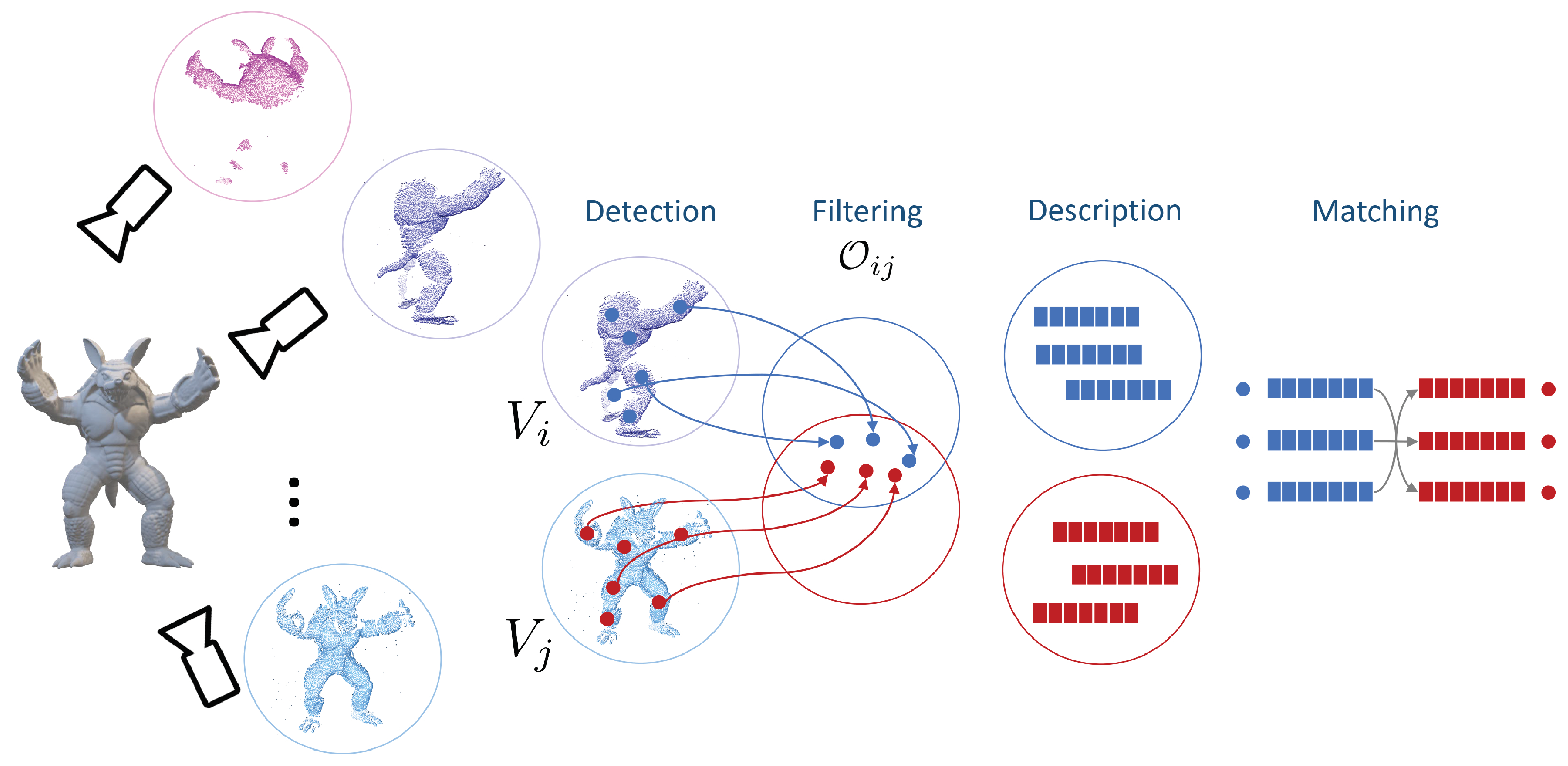
The goal of surface registration is to align into a common 3D reference frame several partial views (usually referred to as scans) of a 3D object obtained by a certain optical sensor. This is achieved through rather complex procedures that, however, typically rely on a key initial step, referred to as Pairwise Registration, aimed at estimating the rigid motion between any two views by a feature-matching pipeline. Thus, in surface registration, 3D feature detection, description and matching are instrumental to attain an as good as possible set of pairwise alignments between the views which then undergoes further processing to get the final global alignment. Differently from object recognition scenarios, the main nuisances deal with missing regions, self-occlusions, limited overlap area between views and point density variations. An overview of how pair-wise correspondences are attained in a typical surface registration pipeline is depicted in Figure 2.
Thus, given a set of M real scans available for a test model, we compute all the possible view pairs . For each pair, we run keypoint detection on both views. Due the partial overlap between the views, a keypoint belonging to may have no correspondence in . Hence, denoted as and the ground-truth transformations that, respectively, bring and into a canonical reference frame, we can compute the set that contains the keypoints in that have a corresponding point in . In particular, given a keypoint :
where denotes the nearest neighbor of in the transformed view . If the number of points in is less than 20% of the keypoints in , the pair is not considered in the evaluation experiments due to insufficient overlap. Conversely, for all the view pairs exhibiting sufficient overlap, a list of correspondences between all the keypoints detected in and all the keypoints extracted from is established by finding the nearest neighbor in the descriptor space via kd-tree matching. Then, given a pair of matched keypoints , , the set of correct correspondences, , can be identified based on the available ground-truth transformations by checking whether the matched keypoints lay within a certain distance in the canonical reference frame:
Then, the precision of the matching process can be computed as a function of the distance threshold [14]:
The precision score associated with any given model is obtained by averaging across all view pairs. We also average across all test models so as to get the final score associated the Laser Scanner dataset.
Eventually, we point out that rather than showing the precision as a function of the distance threshold , we provide the score for a fixed and tight distance threshold value, the same value used to establish upon correctness of matches in object recognition experiments. Indeed, as highlighted in [14], the truly meaningful precision score is that dealing with a distance threshold tight enough to sift out useful correspondences in the addressed scenario. According to our experience, the adopted common threshold for the object recognition and surface registration experiments fulfills this requirement in both settings. Moreover, we think that having the same threshold value in both experiments renders the results more easily comparable.
2.2.3. Datasets
Akin to [5], in our experiments on object recognition we rely on the following popular datasets (see also Figure 3):
- UWA dataset, introduced by Mian et al. [34]. This dataset consists of 4 full 3D models and 50 scenes wherein models significantly occlude each other. To create some clutter, scenes contain also an object which is not included in the model gallery. As scenes are scanned by a Minolta Vivid 910 scanner, they are corrupted by real sensor noise.
- Random Views dataset, based on the Stanford 3D scanning repository (3 http://graphics.stanford.edu/data/3Dscanrep/ accessed on 14 November 2020) and originally proposed in [1]. This dataset comprises 6 full 3D models and 36 scenes obtained by synthetic renderings of random model arrangements. Scenes feature occlusions but no clutter. Moreover, scenes are corrupted by different levels of synthetic noise. In the experiments we consider scenes with Gaussian noise equal to mesh resolution units.
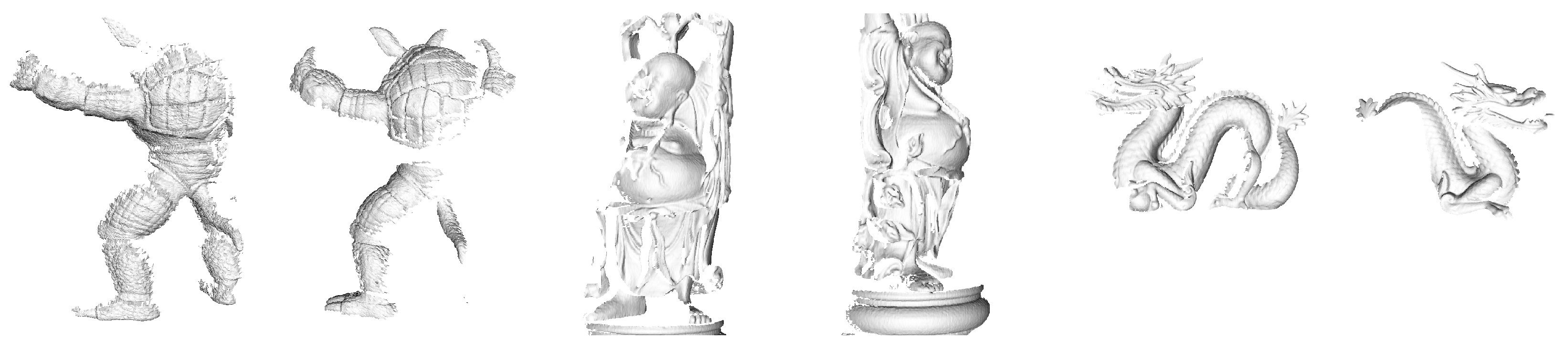
As far as surface registration is concerned, we use the Laser Scanner dataset, proposed in [14]. This dataset includes 8 public-domain 3D models, i.e., 3 taken from the AIM@SHAPE repository (Bimba, Dancing Children and Chinese Dragon), 4 from the Stanford 3D Scanning Repository (Armadillo, Buddha, Bunny, Stanford Dragon) and Berkeley Angel [35]. According to the protocol described in [14], training should be carried out based on synthetic views generated from Berkeley Angel, Bimba, Bunny and Chinese Dragon, while the test data consists of the the real scans available for the remaining 3 models (Armadillo, Buddha and Stanford Dragon). Figure 4 reports exemplar scans from the Laser Scanner test set. We follow the split into train and test objects proposed by the authors.
2.2.4. Implementation
For all handcrafted descriptors considered in our evaluation, i.e., FPFH, ROPS, SHOT, SI, and USC, we use the implementation available in PCL [36], which relies on the original parameter settings proposed by the authors. As for the learned descriptor, i.e., CGF-32, we use the public implementation made available by the authors [14]. As for the Keypoint Learning (KPL) framework described in Section 2.1, we use the publicly available original code for the generation of the training set (http://github.com/CVLAB-Unibo/Keypoint-Learning accessed on 14 November 2020.) together with the OpenCV (opencv.org) implementation of Random Forest classifier. We also keep all the KPL hyperparameters to the values proposed by the authors in [5]. Accordingly, each Forest consists of 100 trees of maximum depth equal to 25 while the minimum number of samples to stop splitting a node is 1. During the detection phase, each point of an unseen point cloud is passed through the Random Forest classifier which produces a score. A point is identified as a keypoint if it exhibits a local maximum of the scores in a neighborhood of radius and the score is higher than a threshold .
For each descriptor considered in our evaluation, we train its paired detector according to the KPL framework. As a result, we obtain six detector-descriptor pairs, referred to from now on as KPL-CGF32, KPL-FPFH, KPL-ROPS, KPL-SHOT, KPL-SI, KPL-USC.
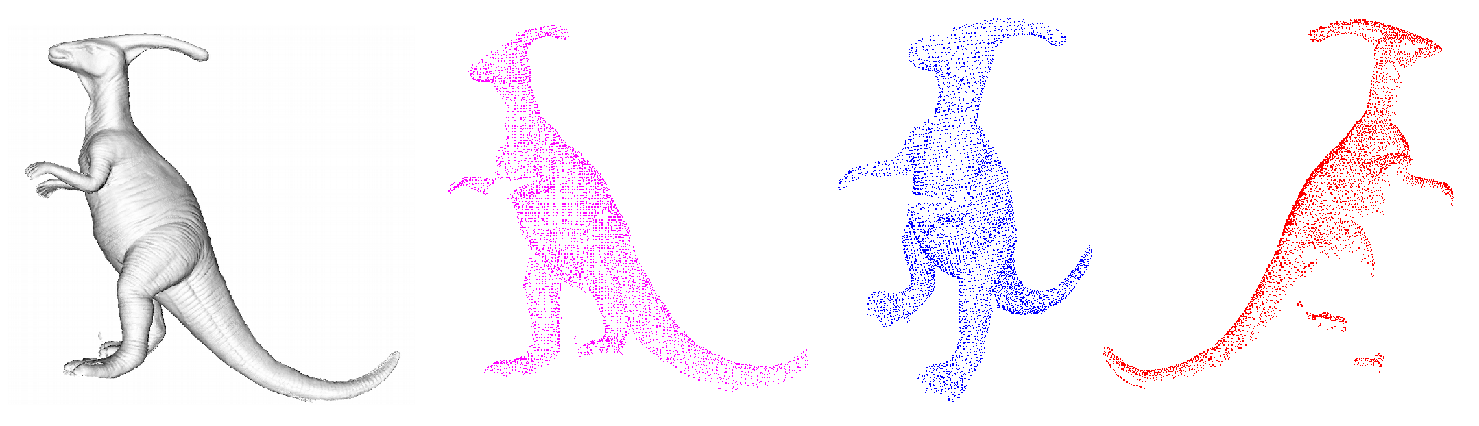
In object recognition experiments, the training data for all detectors are generated from the 4 full 3D models present in the UWA dataset. Purposely, according to the KPL methodology [4,5], for each model we render views from the nodes of an icosahedron centered at the centroid. Some of the generated views are presented in the Figure 5.
Then, the detectors are used in the scenes of the UWA dataset as well as in those of the Random Views dataset. Thus, similarly to [4,5], we do not retrain the detectors on Random Views in order to test the ability of the considered detector-descriptor pairs to generalize well to unseen models in object recognition settings. A coherent approach was pursued for the CGF-32 descriptor. As the authors do not provide a model trained on the UWA dataset, we trained the descriptor on the synthetically rendered views of the 4 UWA models using the code provided by the authors and following the protocol described in the paper in order to generate the data needed by their learning framework based on the triplet ranking loss. Thus, KPL-CGF32 was trained on UWA models and, like all other detector-descriptor pairs, tested on both UWA and Random Views scenes.
In surface registration experiments we proceed according to the protocol proposed in [14]. Hence, detectors are trained with rendered views of the train models provided within the Laser Scanner dataset (Angel, Bimba, Bunny, Chinese Dragon) and tested on the real scans of the test models (Armadillo, Buddha, Stanford Dragon). As CGF-32 was trained exactly on the above mentioned train models [14], to carry out surface registration experiments we did not retrain the descriptor but used the trained network published by the authors (https://github.com/marckhoury/CGF accessed on 14 November 2020).
The values of the main parameters of the detector-descriptor pairs used in the experiments are summarized in Table 1 and Table 2. Accordingly to [5], we used the same support size for all descriptors and all detectors across all the datasets. As it can be observed from Table 1, train parameters for Random Views dataset are not specified as we did not train a new KPL detector on this dataset.
As regards the parameters used in surface registration, since models belong to different repository, we report parameters grouped by model. Test parameters for Angel, Bimba, Bunny and Chinese Dragon are not reported as they are only used in train. Similarly, we omit train parameters for Armadillo, Buddha and Stanford Dragon. Due to the different shape of the models in the dataset, is tuned during the train stage so that the number of overlapping views remains constant across all models.
3. Results and Discussion
In this section, we report experimental results and discuss them. Compared to the most recent evaluation in the field [2], our results allow to assess the performance of the recently proposed KPL methodology based on machine learning as a keypoint detector (which is not considered in [2]) when paired with descriptors or when tested on datasets not considered in [5]. Moreover, we also include a learned descriptor (CGF) in the pool of compared methods, while [2] only consider hand-crafted methods. The main limitation of our study is the smaller number of datasets and acquisition modalities with respect to [2], although on the other hand we rely on real partial scans for the surface registration experiment, while only one synthetic dataset, obtained by creating virtual views of the UWA dataset model gallery, is used in [2].
3.1. Object Recognition
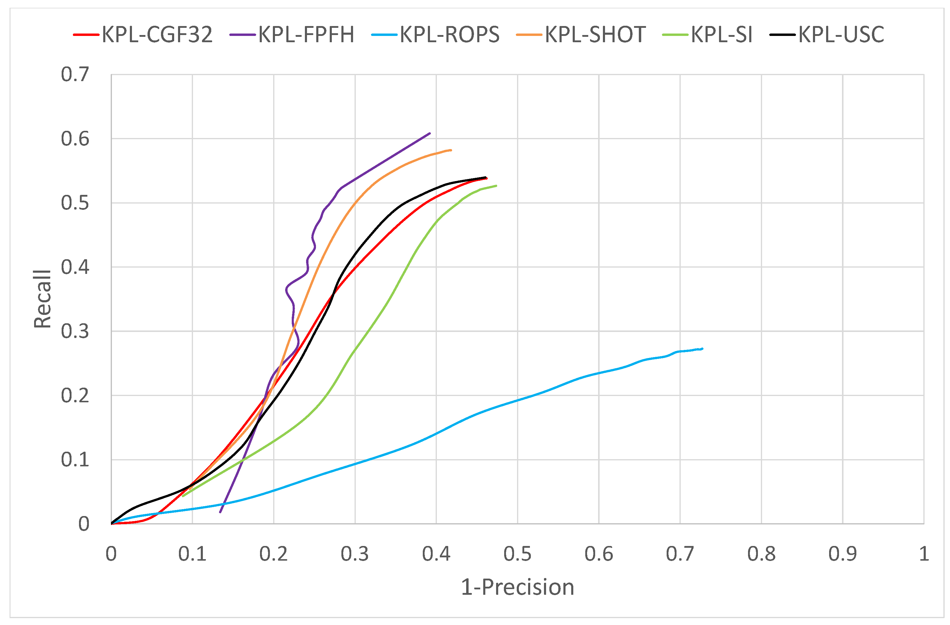
The results on the UWA dataset are shown in Figure 6. First, we wish to highlight how the features based on descriptors which encode just the spatial densities of points around a keypoint outperform those relying on higher order geometrical attributes (such as, e.g., normals). Indeed, KPL-CGF32, KPL-USC and KPL-SI yield significantly better results than KPL-SHOT and KPL-FPFH. These results are coherent with the findings and analysis reported in the performance evaluation by Guo et al. [2], which pointed out the former feature category being more robust to clutter and sensor noise. It is also worth observing how the representation based on the spatial tessellation and point density measurements proposed in [16] together with the local reference frame proposed in [6] turn out particularly amenable to object recognition, as it is actually deployed by both features yielding neatly the best performance, namely KPL-CGF32 and KPL-USC. Yet, learning a dataset-specific non-linear mapping by a deep neural network on top of this good representation does improve performance quite a lot, as vouched by KPL-CGF32 outperforming KPL-USC by a large margin. Indeed, the results obtained in this paper by learning both a dataset-specific descriptor as well as its paired optional detector, i.e., the features referred to as KPL-CGF32, turn out significantly superior to those previously published on UWA object recognition dataset (see [4,5]).
In [5], the results achieved on Random Views by the detectors trained on UWA prove the ability of the KPL methodology to learn to detect general rather than dataset-specific local shapes amenable to provide good matches alongside with the paired descriptor, and even more effectively, in fact, than the shapes found by handcrafted detectors. Thus, when comparing the different descriptors, we can assume here that descriptors are computed on the best available patches and results highlight the ability to handle the specific nuisances of the Random Views dataset. As shown in Figure 7, KPL-FPFH and KPL-SHOT outperform KPL-USC, KPL-CGF32 and KPL-SI. Again, this is coherent with previous findings reported in literature (see [2,5]), which show how descriptors based on higher order geometrical attributes turn out more effective on Random Views due to the lack of clutter and real sensor noise. As for KPL-CGF32, although its performances are still overall better than those of the other descriptors based on point densities, we observe quite a remarkable performance drop compared to the UWA dataset, much larger, indeed, than the feature sharing the very same input representation, i.e., KPL-USC. This suggests that the non-linear mapping learnt by KPL-CGF32 is highly optimized to tell apart the features belonging to the objects present in the training dataset (i.e., UWA) but turn out quite less effective when applied to unseen features, like those found on the objects belonging to Random Views. This domain shift issue is quite common to learned representations and may yield to less stable performance across different datasets than handcrafted representations.
3.2. Surface Registration
First, we deem it worth pointing out how, unlike object recognition settings, in surface registration it is never possible to train any supervised machine learning operator, either detector or descriptor, on the very same objects that would then be processed at test time. Indeed, should one be given either a full 3D model or a set of scans endowed with ground-truth transformations, as required to train 3D feature detectors (i.e., KPL) or descriptors (e.g., CGF-32), there would be no need to carry out any registration for that object. Surface registration is about stitching together several scans of a new object than one wishes to acquire as a full 3D model. As such, any supervised learning machinery is inherently prone to the domain shift issue.
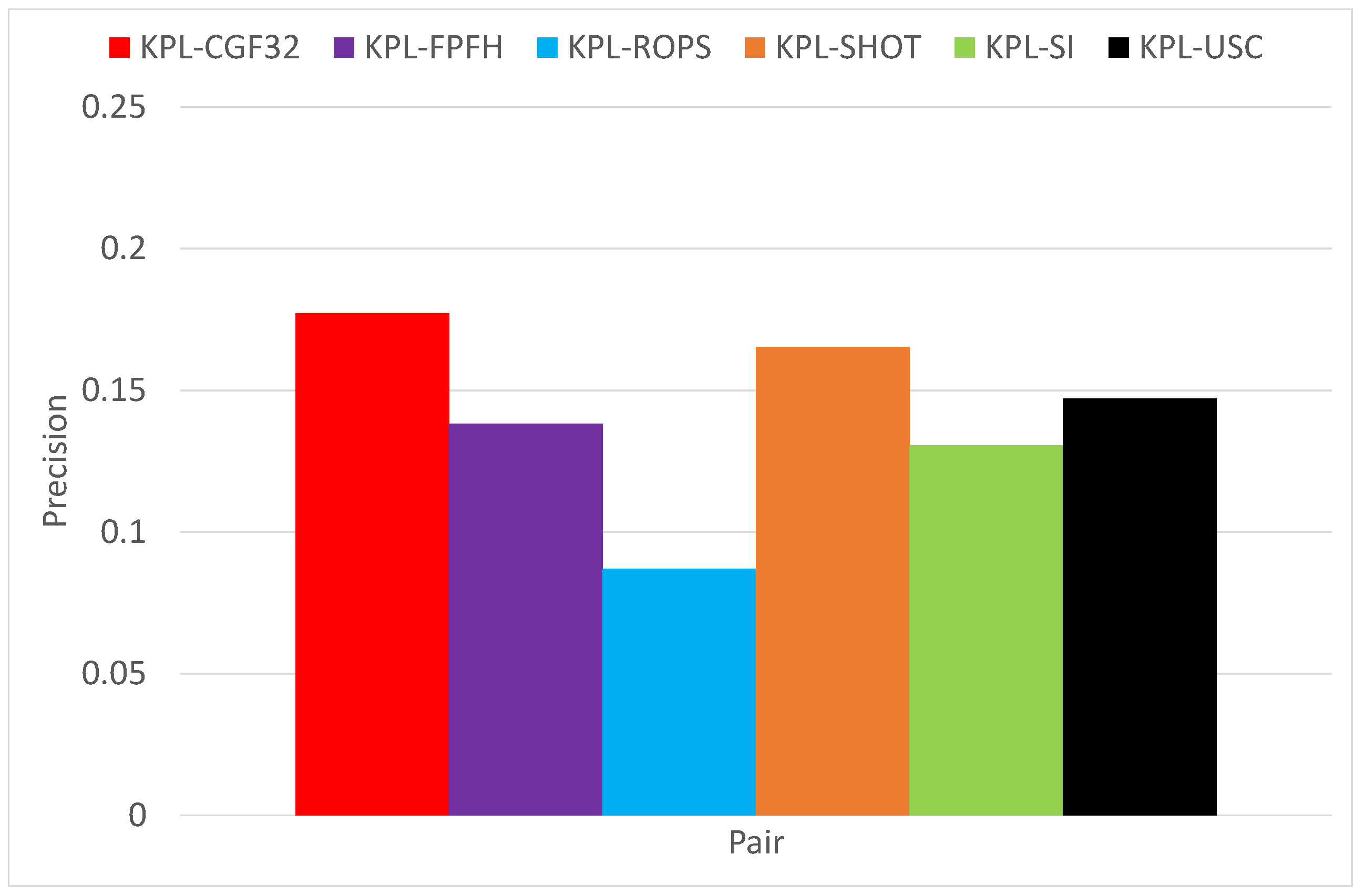
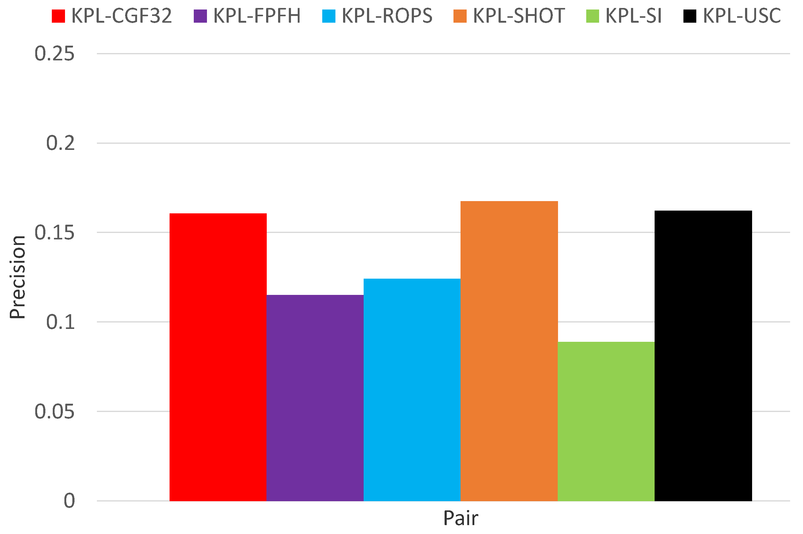
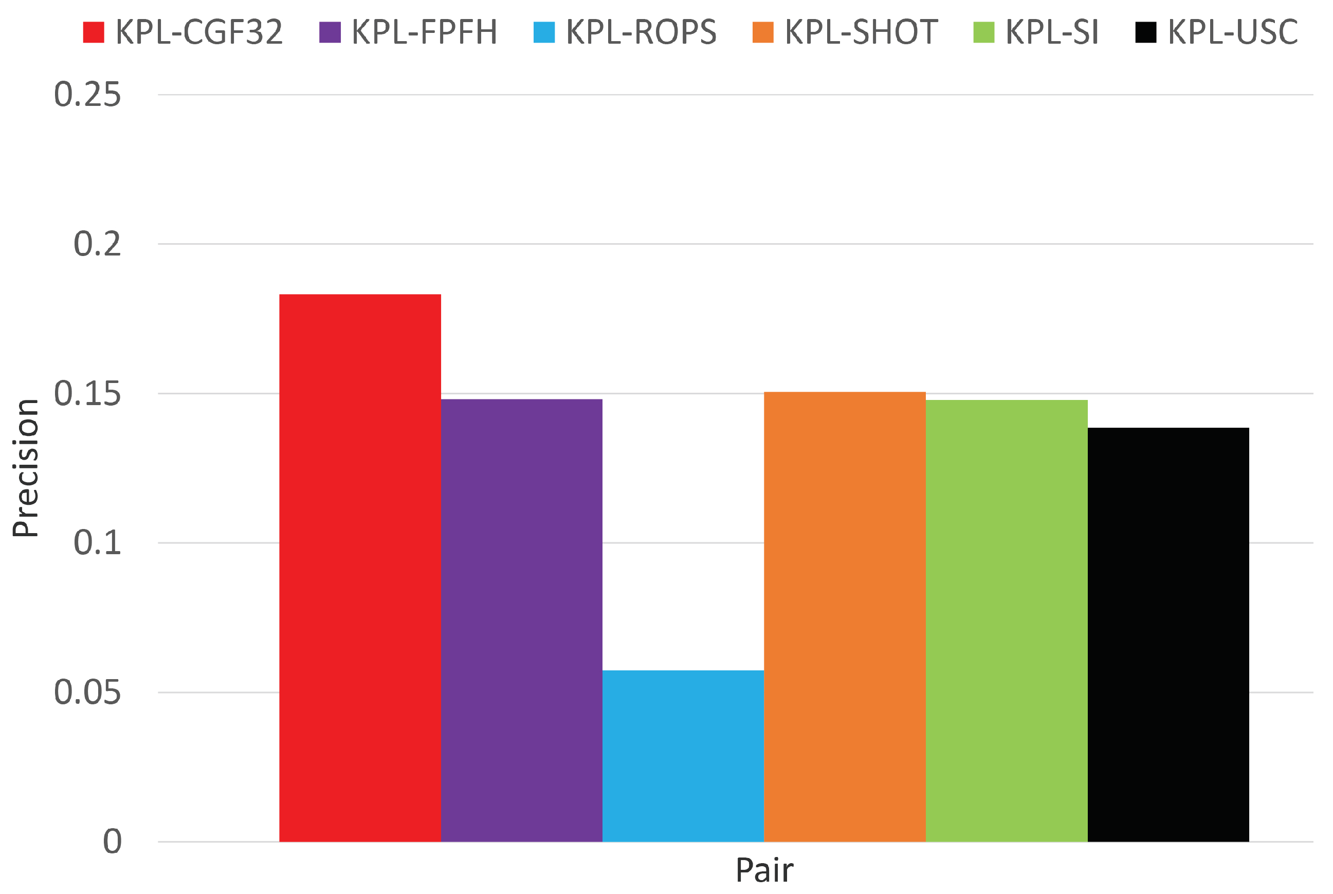
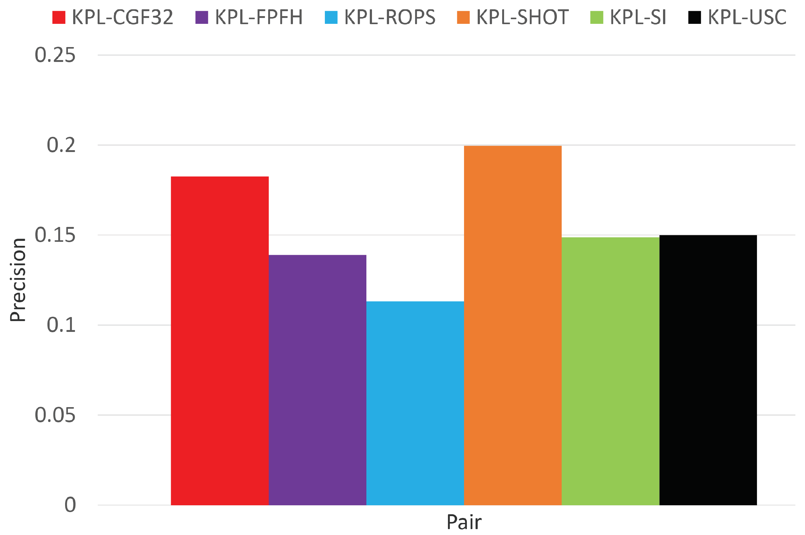
As shown in Figure 8, when averaging across all test objects, the detector-descriptor pair based on the learned descriptor CGF-32 provides the best performance, which confirms the findings reported in [14] where the authors introduce CGF-32 and prove its good registration performance on Laser Scanner. It is worth highlighting here that, as we evaluate detector-descriptor pairs, our results are determined by both the repeatability of the detector as well as the effectiveness of the descriptor, whilst the registration experiments in [14], according to the established descriptor evaluation methodology (e.g., [2,6]) assume an ideal feature detector, i.e., the feature points are mapped from one view into another by the available ground-truth transformation. This different experimental settings explain the difference between the precision values in Figure 8 and those reported in [14]. Figure 8 shows also that, compared to the features based on handcrafted descriptors, and in particular KPL-SHOT, the gain provided by KPL-CGF32 is not as substantial as we did found in object recognition experiments (see Figure 6). Moreover, looking at the results on the individual test objects, reported in Figure 9, Figure 10 and Figure 11, one may observe how KPL-CGF32 outperforms the feature pairs based on handcrafted descriptors only on Buddha, with KPL-SHOT yielding better results on Stanford Dragon and both KPL-SHOT as well as KPL-USC comparing favourably to KPL-CGF32 on Armadillo. This last experiment is particularly interesting due to CGF-32 consisting in a non-linear mapping learnt on top of the input representation deployed by USC. Unlike in object recognition, though, this mapping can only be learnt on different objects than those seen at test time and, hence, because of the domain shift, may not always turn out beneficial.
4. Conclusions and Future Work
Object recognition settings turn out quite amenable to deploy learned 3D features. Indeed, one can train upon a set of 3D objects available beforehand, e.g., due to scanning by some sensor or as CAD models, and then seek to recognize them into scenes featuring occlusions and clutter. These settings allow for learning a highly specialized descriptor alongside its optimal paired detector so to achieve excellent performance. In particular, the learned pair referred to in this paper as KPL-CGF32 sets the new state of the art on the UWA benchmark dataset, being able to achieve 0.45 recall at 0.8 precision. Although the learned representation may not exhibit comparable performance when transferred to unseen objects, in object recognition it is always possible to retrain on the objects at hand to improve performance. An open question left to future work concerns whether the input parametrization deployed by CGF-32 may enable to learn an highly effective non-linear mapping also in datasets characterized by different nuisances (e.g., Laser Scanner) or one should better try to learn 3D representations directly from raw data, as vouched by the success of deep learning from image recognition. Features based on learned representations, such as KPL-CGF32, are quite effective also in surface registration, where it delivers 0.18 precision on the Laser Scanner dataset, the highest value attained in our study, although this scenario is inherently more prone to the domain shift issue such that features based on handcrafted descriptors, like in particular KPL-SHOT and KPL-USC, turn out still very competitive and delivers similar performance (0.16 precision for the former on the same dataset).
We believe that these findings may pave the way for further research on the recent field of learned 3D representations, in particular in order to foster addressing domain adaptation issues, a topic investigated more and more intensively in nowadays deep learning literature concerned with image recognition (see e.g., [37]). Indeed, 3D data are remarkably diverse in nature due to the variety of sensing principles and related technologies and we witness a lack of large training datasets, e.g., at a scale somehow comparable to ImageNet, that may allow learning representations from a rich and varied corpus of 3D models. Therefore, how to effectively transfer learned representations to new scenarios seems a key issue to the success of machine/deep learning in the most challenging 3D Computer Vision tasks.
Finally, KPL has established a new framework whereby one can learn an optimal detector for any given descriptor. In this paper we have shown how applying KPL to a learned representation (CGF-32) leads to particularly effective features (KPL-CGF32), in particular when pursuing object recognition. Yet, according to the KPL training protocol, the descriptor (e.g., CGF-32) has to be learnt before its paired detector: one might be willing to investigate on whether and how a single end-to-end paradigm may allow learning both components jointly so as to further improve performance.
Author Contributions
Conceptualization, R.S. and L.D.S.; Methodology, R.S.; software, R.S.; validation, R.S., S.S. and L.D.S.; investigation, R.S., S.S. and L.D.S.; resources, L.D.S.; data curation, R.S. and S.S.; writing—original draft preparation, R.S.; writing—review and editing, S.S. and L.D.S.; visualization, R.S.; supervision, S.S. and L.D.S.; project administration, L.D.S.; funding acquisition, L.D.S. All authors have read and agreed to the published version of the manuscript.
Funding
This research received no external funding.
Conflicts of Interest
The authors declare no conflict of interest.
References
- Tombari, F.; Salti, S.; Di Stefano, L. Performance evaluation of 3D keypoint detectors. Int. J. Comput. Vis. 2013, 102, 198–220. [Google Scholar] [CrossRef]
- Guo, Y.; Bennamoun, M.; Sohel, F.; Lu, M.; Wan, J.; Kwok, N.M. A comprehensive performance evaluation of 3D local feature descriptors. Int. J. Comput. Vis. 2016, 116, 66–89. [Google Scholar] [CrossRef]
- Salti, S.; Petrelli, A.; Tombari, F.; Di Stefano, L. On the affinity between 3D detectors and descriptors. In Proceedings of the 2012 Second International Conference on 3D Imaging, Modeling, Processing, Visualization & Transmission, Zurich, Switzerland, 13–15 October 2012; pp. 424–431. [Google Scholar]
- Salti, S.; Tombari, F.; Spezialetti, R.; Di Stefano, L. Learning a descriptor-specific 3d keypoint detector. In Proceedings of the IEEE International Conference on Computer Vision, Santiago, Chile, 11–18 December 2015; pp. 2318–2326. [Google Scholar]
- Tonioni, A.; Salti, S.; Tombari, F.; Spezialetti, R.; Di Stefano, L. Learning to Detect Good 3D Keypoints. Int. J. Comput. Vis. 2018, 126, 1–20. [Google Scholar] [CrossRef]
- Tombari, F.; Salti, S.; Di Stefano, L. Unique Signatures of Histograms for Local Surface Description. In Proceedings of the 11th European Conference on Computer Vision Conference on Computer Vision: Part III, Crete, Greece, 5–11 September 2010; Springer: Berlin/Heidelberg, Germany, 2010; pp. 356–369. [Google Scholar]
- Johnson, A.E.; Hebert, M. Using spin images for efficient object recognition in cluttered 3D scenes. IEEE Trans. Pattern Anal. Mach. Intell. 1999, 21, 433–449. [Google Scholar] [CrossRef] [Green Version]
- Rusu, R.B.; Bradski, G.; Thibaux, R.; Hsu, J. Fast 3d recognition and pose using the viewpoint feature histogram. In Proceedings of the 2010 IEEE/RSJ International Conference on Intelligent Robots and Systems, Taipei, Taiwan, 18–22 October 2010; pp. 2155–2162. [Google Scholar]
- Zhong, Y. Intrinsic shape signatures: A shape descriptor for 3d object recognition. In Proceedings of the 2009 IEEE 12th International Conference on Computer Vision Workshops, ICCV Workshops, Kyoto, Japan, 27 September–4 October 2009; pp. 689–696. [Google Scholar]
- Sipiran, I.; Bustos, B. Harris 3D: A robust extension of the Harris operator for interest point detection on 3D meshes. Vis. Comput. 2011, 27, 963. [Google Scholar] [CrossRef]
- Steder, B.; Rusu, R.B.; Konolige, K.; Burgard, W. NARF: 3D range image features for object recognition. In Workshop on Defining and Solving Realistic Perception Problems in Personal Robotics at the IEEE/RSJ Int. Conf. on Intelligent Robots and Systems (IROS); 2010; Volume 44, Available online: https://www.researchgate.net/publication/260320178_NARF_3D_Range_Image_Features_for_Object_Recognition?enrichId=rgreq-8976992b9b5ce6b1365b18388cdf9865-XXX&enrichSource=Y292ZXJQYWdlOzI2MDMyMDE3ODtBUzoxODU1NjExNjM3NzE5MDhAMTQyMTI1MjYzNzk5MQ%3D%3D&el=1_x_2&_esc=publicationCoverPdf (accessed on 20 November 2020).
- Tombari, F.; Salti, S.; Di Stefano, L. Unique shape context for 3D data description. In Proceedings of the ACM Workshop on 3D Object Retrieval, Firenze, Italy, 25–29 October 2010; pp. 57–62. [Google Scholar]
- Guo, Y.; Sohel, F.; Bennamoun, M.; Lu, M.; Wan, J. Rotational projection statistics for 3D local surface description and object recognition. Int. J. Comput. Vis. 2013, 105, 63–86. [Google Scholar] [CrossRef] [Green Version]
- Khoury, M.; Zhou, Q.Y.; Koltun, V. Learning compact geometric features. In Proceedings of the IEEE Conference on Computer Vision and Pattern Recognition, Honolulu, HI, USA, 21–26 July 2017; pp. 153–161. [Google Scholar]
- Harris, C.; Stephens, M. A combined corner and edge detector. In Alvey Vision Conference; Citeseer: University Park, PA, USA, 1988; Volume 15, pp. 10–5244. [Google Scholar]
- Frome, A.; Huber, D.; Kolluri, R.; Bülow, T.; Malik, J. Recognizing objects in range data using regional point descriptors. In European Conference on Computer Vision; Springer: New York, NY, USA, 2004; pp. 224–237. [Google Scholar]
- Rusu, R.B.; Blodow, N.; Marton, Z.C.; Beetz, M. Aligning point cloud views using persistent feature histograms. In Proceedings of the 2008 IEEE/RSJ International Conference on Intelligent Robots and Systems, Nice, France, 22–26 September 2008; pp. 3384–3391. [Google Scholar]
- Zeng, A.; Song, S.; Nießner, M.; Fisher, M.; Xiao, J.; Funkhouser, T. 3dmatch: Learning local geometric descriptors from rgb-d reconstructions. In Proceedings of the 2017 IEEE Conference on Computer Vision and Pattern Recognition (CVPR), Honolulu, HI, USA, 21–26 July 2017; pp. 199–208. [Google Scholar]
- Gojcic, Z.; Zhou, C.; Wegner, J.D.; Andreas, W. The Perfect Match: 3D Point Cloud Matching with Smoothed Densities. In Proceedings of the International Conference on Computer Vision and Pattern Recognition (CVPR), Long Beach, CA, USA, 16–20 June 2019. [Google Scholar]
- Qi, C.R.; Su, H.; Mo, K.; Guibas, L.J. Pointnet: Deep learning on point sets for 3d classification and segmentation. In Proceedings of the IEEE Conference on Computer Vision and Pattern Recognition (CVPR), Honolulu, HI, USA, 21–26 July 2017. [Google Scholar]
- Weinberger, K.Q.; Saul, L.K. Distance metric learning for large margin nearest neighbor classification. J. Mach. Learn. Res. 2009, 10, 207–244. [Google Scholar]
- Schultz, M.; Joachims, T. Learning a distance metric from relative comparisons. In Advances in Neural Information Processing Systems; Springer: New York, NY, USA, 2004; pp. 41–48. [Google Scholar]
- Li, L.; Zhu, S.; Fu, H.; Tan, P.; Tai, C.L. End-to-End Learning Local Multi-view Descriptors for 3D Point Clouds. In Proceedings of the IEEE/CVF Conference on Computer Vision and Pattern Recognition, Seattle, WA, USA, 14–19 June 2020; pp. 1919–1928. [Google Scholar]
- Deng, H.; Birdal, T.; Ilic, S. PPF-FoldNet: Unsupervised Learning of Rotation Invariant 3D Local Descriptors. In Proceedings of the European Conference on Computer Vision (ECCV), Munich, Germany, 8–14 September 2018; pp. 602–618. [Google Scholar]
- Zhao, Y.; Birdal, T.; Deng, H.; Tombari, F. 3D Point Capsule Networks. In Proceedings of the Conference on Computer Vision and Pattern Recognition (CVPR), Long Beach, CA, USA, 16–20 June 2019. [Google Scholar]
- Birdal, T.; Ilic, S. Point pair features based object detection and pose estimation revisited. In Proceedings of the 2015 International Conference on 3D Vision, Lyon, France, 19–22 October 2015; pp. 527–535. [Google Scholar]
- Drost, B.; Ulrich, M.; Navab, N.; Ilic, S. Model globally, match locally: Efficient and robust 3D object recognition. In Proceedings of the 2010 IEEE Computer Society Conference on Computer Vision and Pattern Recognition, San Francisco, CA, USA, 13–18 June 2010; pp. 998–1005. [Google Scholar]
- Yang, Y.; Feng, C.; Shen, Y.; Tian, D. FoldingNet: Point Cloud Auto-Encoder via Deep Grid Deformation. In Proceedings of the IEEE Conference on Computer Vision and Pattern Recognition, Salt Lake City, UT, USA, 18–23 June 2018; pp. 206–215. [Google Scholar]
- Spezialetti, R.; Salti, S.; Stefano, L.D. Learning an Effective Equivariant 3D Descriptor Without Supervision. In Proceedings of the IEEE International Conference on Computer Vision (ICCV), Seoul, Korea, 27 October–2 November 2019. [Google Scholar]
- Groueix, T.; Fisher, M.; Kim, V.G.; Russell, B.C.; Aubry, M. A Papier-Mâché Approach to Learning 3D Surface Generation. In Proceedings of the IEEE Conference on Computer Vision and Pattern Recognition, Salt Lake City, UT, USA, 18–22 June 2018; pp. 216–224. [Google Scholar]
- Cohen, T.S.; Geiger, M.; Köhler, J.; Welling, M. Spherical CNNs. arXiv 2018, arXiv:1801.10130. [Google Scholar]
- Breiman, L. Random forests. Mach. Learn. 2001, 45, 5–32. [Google Scholar] [CrossRef] [Green Version]
- Teran, L.; Mordohai, P. 3d interest point detection via discriminative learning. In European Conference on Computer Vision; Springer: New York, NY, USA, 2014; pp. 159–173. [Google Scholar]
- Mian, A.; Bennamoun, M.; Owens, R. On the repeatability and quality of keypoints for local feature-based 3d object retrieval from cluttered scenes. Int. J. Comput. Vis. 2010, 89, 348–361. [Google Scholar] [CrossRef] [Green Version]
- Kolluri, R.; Shewchuk, J.R.; O’Brien, J.F. Spectral surface reconstruction from noisy point clouds. In Proceedings of the 2004 Eurographics/ACM SIGGRAPH Symposium on Geometry Processing; ACM: New York, NY, USA, 2004; pp. 11–21. [Google Scholar]
- Rusu, R.B.; Cousins, S. 3d is here: Point cloud library (pcl). In Proceedings of the 2011 IEEE International Conference on Robotics and Automation, Shanghai, China, 9–13 May 2011; pp. 1–4. [Google Scholar]
- Wang, M.; Deng, W. Deep Visual Domain Adaptation: A Survey. Neurocomputing 2018, 312, 135–153. [Google Scholar] [CrossRef] [Green Version]
Figure 1.
Overview of the local feature matching pipeline for 3D object recognition.

Figure 2.
Overview of the local feature matching pipeline for surface registration.

Figure 3.
Scene from the UWA (left) and Random Views (right) datasets.

Figure 4.
Laser Scanner dataset: scans from Armadillo, Buddha and Stanford Dragon.

Figure 5.
A 3D model and some rendered views from UWA.

Figure 6.
Object recognition results on UWA dataset.

Figure 7.
Object recognition results on Random Views dataset.

Figure 8.
Surface registration results on the Laser Scanner dataset.

Figure 9.
Surface registration results on Armadillo.

Figure 10.
Surface registration results on Buddha.

Figure 11.
Surface registration results on Stanford Dragon.


Table 1.
Parameters for object recognition datasets. All metric values are in millimeters.
| Dataset | ||||||||
|---|---|---|---|---|---|---|---|---|
| UWA | 40 | 20 | 0.85 | 7 | 4 | 2 | 4 | 0.8 |
| Random Views | 40 | 20 | - | 7 | - | - | 4 | 0.8 |
Table 2.
Parameters for surface registration dataset. All metric values are in millimeters.
| Model Name | |||||||||
|---|---|---|---|---|---|---|---|---|---|
| Angel | 40 | 20 | 0.85 | 7 | 4 | 2 | - | - | - |
| Bimba | 40 | 20 | 0.85 | 7 | 4 | 2 | - | - | - |
| Bunny | 40 | 20 | 0.65 | 7 | 4 | 2 | - | - | - |
| Chinese Dragon | 40 | 20 | 0.65 | 7 | 4 | 2 | - | - | - |
| Armadillo | 40 | 20 | - | 7 | - | - | 2 | 4 | 0.5 |
| Buddha | 40 | 20 | - | 7 | - | - | 2 | 4 | 0.5 |
| Stanford Dragon | 40 | 20 | - | 7 | - | - | 2 | 4 | 0.5 |
Publisher’s Note: MDPI stays neutral with regard to jurisdictional claims in published maps and institutional affiliations. |
© 2021 by the authors. Licensee MDPI, Basel, Switzerland. This article is an open access article distributed under the terms and conditions of the Creative Commons Attribution (CC BY) license (https://creativecommons.org/licenses/by/4.0/).
Share and Cite
MDPI and ACS Style
Spezialetti, R.; Salti, S.; Di Stefano, L. Performance Evaluation of 3D Descriptors Paired with Learned Keypoint Detectors. AI 2021, 2, 229-243. https://0-doi-org.brum.beds.ac.uk/10.3390/ai2020014
AMA Style
Spezialetti R, Salti S, Di Stefano L. Performance Evaluation of 3D Descriptors Paired with Learned Keypoint Detectors. AI. 2021; 2(2):229-243. https://0-doi-org.brum.beds.ac.uk/10.3390/ai2020014
Chicago/Turabian StyleSpezialetti, Riccardo, Samuele Salti, and Luigi Di Stefano. 2021. "Performance Evaluation of 3D Descriptors Paired with Learned Keypoint Detectors" AI 2, no. 2: 229-243. https://0-doi-org.brum.beds.ac.uk/10.3390/ai2020014