What Is the Impact of Heatwaves on European Viticulture? A Modelling Assessment


1
Centre for the Research and Technology of Agro-Environmental and Biological Sciences, CITAB, Universidade de Trás-os-Montes e Alto Douro, UTAD, 5000-801 Vila Real, Portugal
2
Luxembourg Institute of Science and Technology (LIST), Environmental Research and Innovation (ERIN) Department, 41, rue du Brill, L-4422 Belvaux, Luxembourg
3
Department of Agriculture, Food, Environment and Forestry (DAGRI), University of Florence, Piazzale delle Cascine 18, 50144 Florence, Italy
*
Authors to whom correspondence should be addressed.
Appl. Sci. 2020, 10(9), 3030; https://0-doi-org.brum.beds.ac.uk/10.3390/app10093030
Submission received: 7 April 2020
/
Revised: 22 April 2020
/
Accepted: 24 April 2020
/
Published: 26 April 2020
(This article belongs to the Special Issue Climate Change Impact on Viticulture and Potential Adaptation Strategies)
Abstract
:Extreme heat events or heatwaves can be particularly harmful to grapevines, posing a major challenge to winegrowers in Europe. The present study is focused on the application of the crop model STICS to assess the potential impacts of heatwaves over some of the most renowned winemaking regions in Europe. For this purpose, STICS was applied to grapevines, using high-resolution weather, soil and terrain datasets from 1986 to 2015. To assess the impact of heatwaves, the weather dataset was artificially modified, generating periods with anomalously high temperatures (+5 °C), at specific onset dates and with specific episode durations (from five to nine days). The model was then run with this modified weather dataset, and the results were compared to the original unmodified runs. The results show that heatwaves can have a very strong impact on grapevine yields. However, these impacts strongly depend on the onset dates and duration of the heatwaves. The highest negative impacts may result in a decrease in the yield by up to −35% in some regions. The results show that regions with a peak vulnerability on 1 August will be more negatively impacted than other regions. Furthermore, the geographical representation of yield reduction hints at a latitudinal gradient in the heatwave impact, indicating stronger reductions in the cooler regions of Central Europe than in the warmer regions of Southern Europe. Despite some uncertainties inherent to the current modelling assessment, the present study highlights the negative impacts of heatwaves on viticultural yields in Europe, which is critical information for stakeholders within the winemaking sector for planning suitable adaptation measures.
1. Introduction
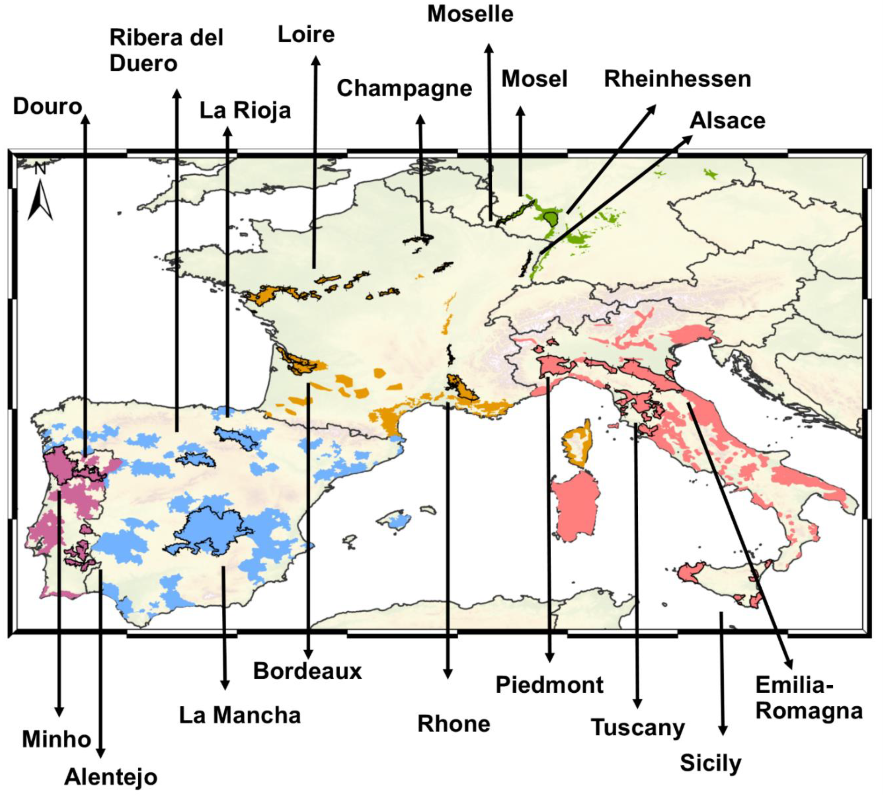
Most of the renowned wine regions in Europe (Figure 1) are characterized by warm temperate climates, namely Mediterranean, oceanic or humid continental [1]. These regions are expected to have pronounced climate change impacts, particularly due to extreme events, such as droughts and extreme heat [2]. Hence, it becomes clear that viticulture is exposed and vulnerable to the change in climatic conditions [3,4], particularly in Southern Europe [5]. Given these threats and their impacts on the vulnerability of grapevine in a warmer world, it is imperative to understand how climate change and extreme events can influence this economically valuable crop in Europe.
Temperature is a key factor affecting plant growth and development rates [6]. For grapevines, air temperature is considered to be a fundamental factor controlling the main physiological processes, phenological timings and overall productivity and quality [7]. Although other atmospheric variables, such as precipitation, humidity and solar radiation, also play an important role in grapevine development, temperature is considered to be the main factor. In effect, grapevine physiology and fruit metabolism/composition are highly influenced by the thermal conditions during the growing season [8]. For adequate grapevine growth, phenological development and yield attributes [9], there are indeed optimum temperature ranges and thermal thresholds, establishing both lower and upper limits, which are, however, variety-dependent. One of the most well-known climatic requirements of the grapevine is the 10 °C base temperature for heat accumulation, which is needed for the onset of its vegetative cycle [10,11,12,13,14,15]. Over the last decades, most research was aimed at the lower thermal limits for heat accumulation, which has traditionally been a major concern for winegrowers. Nonetheless, the effect of high temperatures on grape physiology is likely to become more important in the future, due to global warming [15]. Hence, a better analysis of the upper thermal limits for grape development and physiology is of foremost relevance.
It is known that if air temperature exceeds a given upper threshold (e.g., 35 °C) at certain critical periods of grapevine development, negative impacts on grapevine should be expected [16]. In effect, extreme heat can be particularly harmful to grapevines. Grapevines growing under severe heat stress experience a significant decline in productivity, e.g., due to limitations in photosynthesis [17], as well as injures under other physiological processes [18]. As an example, a study carried out by Matsui et al. [19] concluded that the exposure of Thompson Seedless and Napa Gamay to 40 °C for six consecutive days reduced berry size, as well as sugar accumulation, and delayed ripening. Other studies, for other grapevine varieties exposed to severe heat, showed similar results [20,21]. Furthermore, several physiological processes, such as photosynthesis, are either severely reduced or inhibited at high temperatures (~35 °C), mostly owing to stomatal closure [16,22,23].
The World Meteorological Organization (WMO) defines a heatwave as a weather extreme episode with “5 or more consecutive days of prolonged heat in which the daily maximum temperature is higher than the average maximum temperature by 5 °C or more”. Due to climate change, extreme weather events are projected to increase in frequency, duration and intensity [24]. Combined with the increase in mean temperature projected to occur in the future, heatwaves can indeed be seen as a major challenge that winegrowers will have to deal with in the upcoming decades. As an illustration, the 2003 heatwave in Europe highlighted the potential impact of heatwaves on viticulture [25], particularly during harvest [26]. This record-breaking heatwave in Europe may be seen as a demonstrative extreme event that is expected to occur more frequently under enhanced atmospheric greenhouse gas concentrations and anthropogenic radiative forcing [26,27]. More recently, in 2019, there were three consecutive heatwave events in Europe (in June, July and August), with temperatures reaching 44 °C in some regions during June. Given the risk that heatwaves pose to viticulture and winemaking, a better assessment of the effects of these events on this sector is thereby of the utmost importance.
Crop models can be a valuable tool in assessing the impact of heatwaves on viticulture [28]. These models mechanistically simulate plant development while incorporating weather, soil properties, plant data and management decisions [29]. The simulation of crop parameters, such as yields, under different pedoclimatic conditions, and abiotic stresses, are main outcomes from these models. One of their strongest advantages is the fact that they have already been applied and validated with field measurements, thus reducing the need to provide extensive experimental trials, when properly calibrated and validated. Hence, coupling dynamic (process-based) crop models with high-resolution climate, soil and plant data allows reliable yield simulations over a wide region to be produced. Despite the aforementioned advantages of these models, to our knowledge, their application to understanding the impact of heatwaves on viticulture has not been conducted yet [30].
The present study aims at analyzing the impacts of heatwaves on European viticulture, particularly on grapevine yield. As such, the objectives of the present study are fourfold: (1) to simulate recent-past yields over several main European winemaking regions, using a state-of-the-art crop model for simulating grapevines, forced by observed climate conditions over a past baseline period (control runs); (2) to carry out a sensitivity analysis to heatwaves, applying synthetic heatwave disturbances (heatwave runs); (3) to compute the regional yield differences between control and heatwave runs; and (4) to discuss potential adaptation measures to be implemented by viticulturists and winemakers, to cope with upcoming heatwaves in the near future.
2. Materials and Methods
2.1. Vineyard Locations
The study sites were selected by considering some of the main winegrowing regions in Europe. These regions were selected based on their importance for the current viticultural sector, though not exhaustively. While many other regions in Europe can be considered to be top winemaking regions, they are out of the focus of the current study. The following regions were considered herein (from west to east; Figure 1): Minho, Douro and Alentejo (Portugal); Ribera del Duero, La Rioja and La Mancha (Spain); Bordeaux, Loire Valley, Champagne, Rhone and Alsace (France); Moselle (Luxembourg); Mosel and Rheinhessen (Germany); Piedmont, Tuscany, Sicily and Emilia-Romagna (Italy). All these winemaking regions present temperate climate characteristics [1], despite local and regional specificities. Regarding the annual mean temperatures, these regions typically range from 10 to 17 °C (Table 1), being the coldest regions in the Mosel/Moselle area, in both Germany and Luxembourg, closely followed by Champagne (Northern France), while the warmest is Alentejo (Southern Portugal), followed by Sicily (Southern Italy) and La Mancha (inner Southern Spain). Regarding annual precipitation totals, it roughly varies from 400 to 1000 mm, with Piedmont (Northwestern Italy), Minho (Northwestern Portugal) and Emilia-Romagna (Northern Italy) being the wettest regions, whereas Ribera del Duero (inner Northern Spain), La Mancha and Sicily are the driest regions.
2.2. Crop Model Description
The STICS (Simulateur mulTIdisciplinaire pour les Cultures Standard) crop model, version 121, was used herein to simulate grapevine yields [31]. This model is currently one of the few crop models that incorporates the necessary parameterizations for perennial crops and, more specifically, for grapevine simulations [32,33,34]. In a study by Fraga et al. [35], the STICS model was used to simulate yield, phenology and abiotic (water) stress conditions throughout Europe, showing a high agreement with observational data [35,36]. Subsequently, this model was used in assessing the potential impacts of climate change on viticulture and the effectiveness of different adaptation strategies, like irrigation or mulching [37,38]. The current study follows the same guidelines and parameterizations as in Fraga, et al. [35].
Regarding the model runs, the model operates on a daily time-step, simulating grapevine growth driven by daily weather data. Grapevine budburst is simulated by using the BRIN model [39], whereas flowering and veraison are simulated by using growing degree-days, with a base temperature of 10 °C. To simulate biomass growth, nitrogen and carbon reserves are considered, also taking into account competition between vegetative and generative organs. CO2 effects on plant physiology and radiation use efficiency are also simulated [31]. Fruit growth is described by the dynamics of dry-matter accumulation and water content [40]. Temperature thresholds (i.e., frost and heat shock) are also taken into consideration for growth and development, which is critical for the objectives of the present study.
2.3. Input Data
The model requires a large range of input data, such as daily weather data, typical soil properties, topographic features, varietal characteristics and crop management information. The required daily variables comprise daily maximum air temperature (Tmax), daily minimum air temperature (Tmin), daily accumulation of solar radiation (Rad), daily precipitation total (Prec), daily mean wind speed (Wspeed), daily mean relative humidity (Rh) and CO2 level. These data were obtained from two different observational sources. Tmax, Tmin and Prec were obtained from the E-OBS dataset, version 19e [41], whilst Rad, WSpeed and Rh were retrieved from the ERA5 dataset [42]. These two datasets have been widely used and validated by many previous studies. Data were extracted at 0.1° latitude–longitude regular grids (spatial resolution of approximately 10 km) for the baseline period of 1986–2015.
Soil data, like soil texture and pH, were obtained from the Harmonized World Soil Database HWSD and [43], available from two layers (depths 0–30 cm and 30–100 cm). Some soil properties for STICS were estimated by using pedotransfer functions [44], such as soil albedo, runoff, soil permeability, field capacity, wilting point and bulk density. Additionally, some soil properties were set as standard, following Brisson, et al. [31]: initial soil water content (set at field capacity); maximum unimpeded root depth (200 cm), initial root density (0.05 cm·cm−3) and soil organic N content (6% of dry soil). Terrain data, such as slope degree and orientation, were obtained from the GTOPO30 digital elevation model and using GIS techniques (https://lta.cr.usgs.gov/GTOPO30).
For a large-scale comprehensive modelling approach throughout Europe, some assumptions were made concerning cultivated varieties and cultural practices. As it will not be possible to analyze all the specific varieties grown at each location, which would also impede a comparative analysis among regions, a standard variety was considered for all locations. The selected variety was cv. Pinot noir, due to its early-to-intermediate ripening and moderate yields, being suitable for a large number of viticultural regions [45]. Pinot noir is currently the 10th most planted variety and the 7th fastest-expanding variety in the world [46]. Since it is grown in vineyards throughout Europe, from the warmer countries in Southern Europe to the cooler Central–Northern European wine regions [46], it was chosen herein. Furthermore, this variety was already validated in a previous study [35].
Cultural practices were kept invariant in the model runs, and crop interventions were set to a minimum (i.e., topping, thinning and leaf removal were not considered in the model). The default trellis system was Cordon, and vine density was set to 4000 vines ha-1, a reasonable value considering most commercial vineyards in Europe [47]. The technological harvest date was determined once the berry water content reached a maximum of 77%, corresponding to a probable alcohol level of 12.5 (% v/v) [40].
2.4. Model Runs
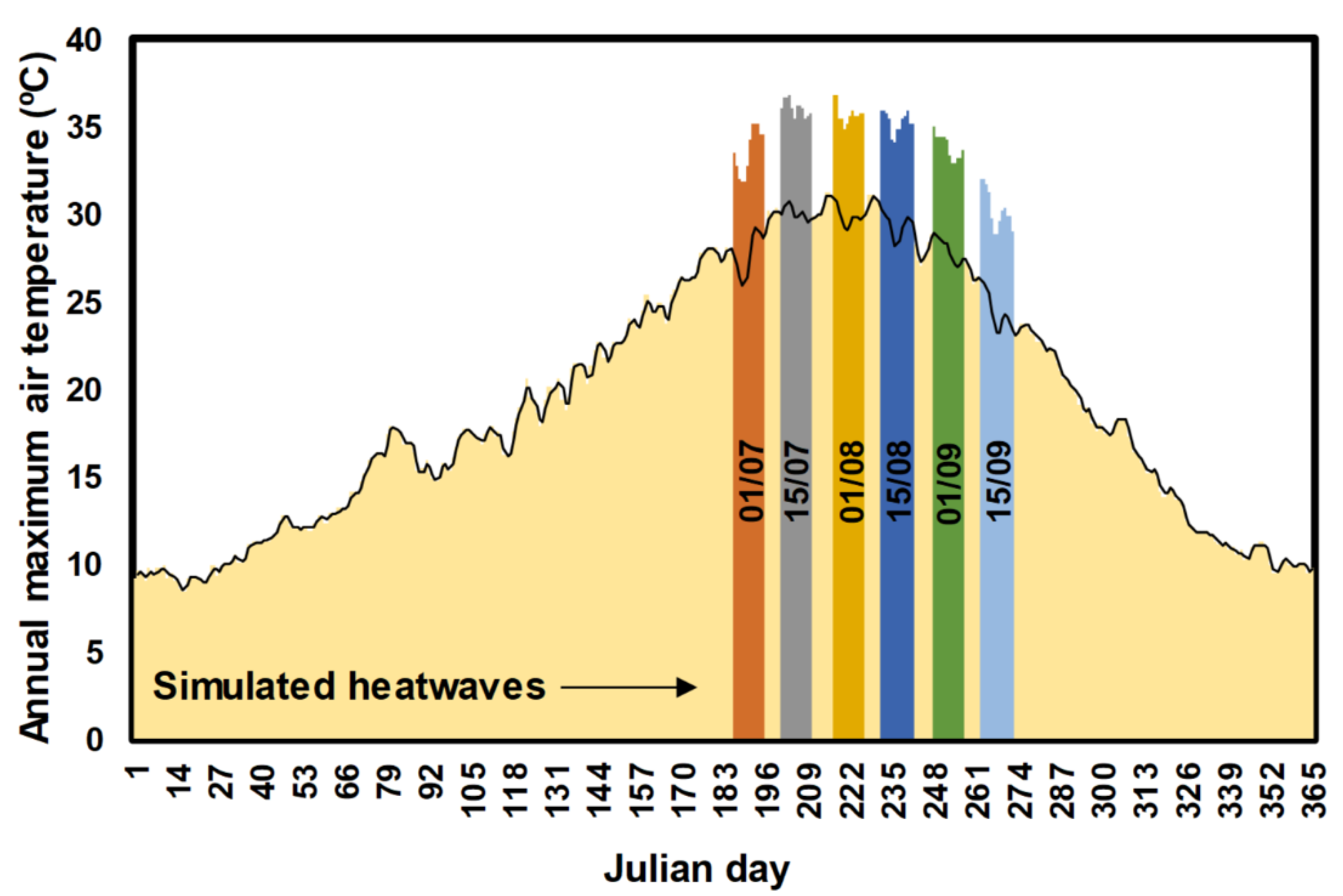
The STICS model was initialized by using the abovementioned input variables. Two types of model runs were performed: control-runs vs. heatwave-runs. The control-run is based on observed conditions, using the observational unmodified weather data. Conversely, for the heatwave-runs, the observed weather conditions were modified, generating heatwave pulses at specific periods of the year and with specific durations (synthetic heatwave disturbances). Therefore, for each year, a heatwave pulse was added to the temperature time series by increasing the daily maximum temperature by 5 ºC with respect to the climatological maximum (following the WMO definition). This change in daily maximum temperature also impacts daily mean temperature. Regarding the onsets of the heatwaves, they were generated with a 15-day leap period, starting on July and ending in September: 1 and 15 July; 1 and 15 August; and 1 and 15 September. Therefore, the most vulnerable period of grapevine exposition to heatwaves is covered. The heatwave then lasted for a period ranging from 5 to 9 days (heatwave length/duration). Only one heatwave per year was considered. During the heatwave, the daily precipitation was set to 0 mm, which is typical during a heatwave. A comprehensive chart of these synthetic heatwaves is shown in Figure 2.
STICS performance under the recent-past conditions has previously been evaluated and revealed good agreement with field data [35]. Thus, the remaining model parameterization followed the previous study [35]. Hence, model runs were carried out for each of the 18 regions, year (30 years; 1986–2015) and type of run (control vs. heatwave), corresponding to a total of 6480 simulations. In order to evaluate the potential impacts of heatwaves on grapevine yields, the heatwave-runs and the control-runs where compared. More specifically, the relative differences (%) in their corresponding yields were analyzed, thus disregarding absolute values and restraining the effects of some uncertainties in the STICS simulations. Nonetheless, it is important to state that the STICS model already showed a high agreement with statistical yields over Europe [35].
3. Results
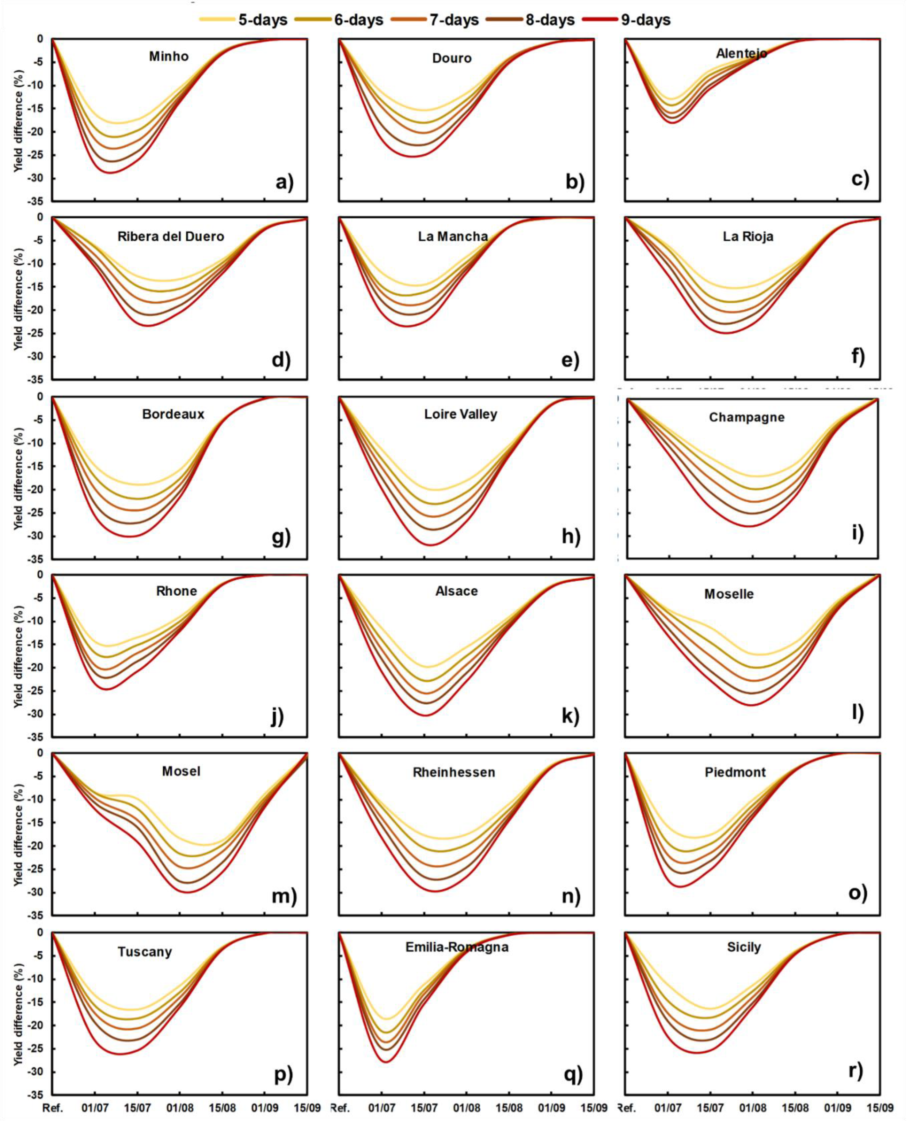
Figure 3 shows the impacts of heatwaves on grapevine yields for each of the selected winemaking regions in Europe. Overall (Figure 3), for all regions, the occurrence of heatwaves will lead to a decrease in yields, with its magnitude increasing along with the heatwave duration. The main differences between these impacts are the maximum yield decrease and the corresponding dates of occurrence of the heatwave vulnerability (heatwave peak, henceforth). Starting with the westernmost regions, for Portugal (Figure 3a–c), all regions reveal a heatwave peak between 1 and 15 July. The region with the strongest decrease in Portugal is Minho, with −15% (five heatwave days) to −29% (nine heatwave days). Conversely, in the Portuguese region of Alentejo, the impacts will not be so pronounced (−12% to −17%). For Spain (Figure 3d–f), La Mancha also shows a peak between 1 and 15 July, while for Ribera del Duero and La Rioja, this peak is expected to occur slightly later, between 15 July and 1 August. Regarding the potential impacts on yield, they will be very similar across these three Spanish wine regions, ranging from −12% to −25%. For the French winemaking regions (Figure 3g–k), the strongest impacts will occur in the Loire Valley and Alsace, reaching −30%, while Rhone will be the region with the lowest negative impacts, with −25%. All regions will tend to show the heatwave peak for 15 July, except in Champagne, which will occur on 1 August. Owing to their geographical proximity, the Luxembourgish region of Moselle (Figure 3l) and the German region of Mosel (Figure 3m) show very similar impacts. Both regions show peak dates around 1 August and impacts from −15% to 30%. Similar results can be observed for Rheinhessen, also due to their fairly identical climatic conditions (Figure 3n). For the Italian regions (Figure 3o–r), the impacts vary from −15% and −27%. All regions will tend to have their peak dates from the 1 July to 15 July. It is worth noting that Emilia-Romagna (Figure 3q) depicts a comparatively narrow curve, which is very concentrated around the peak date.
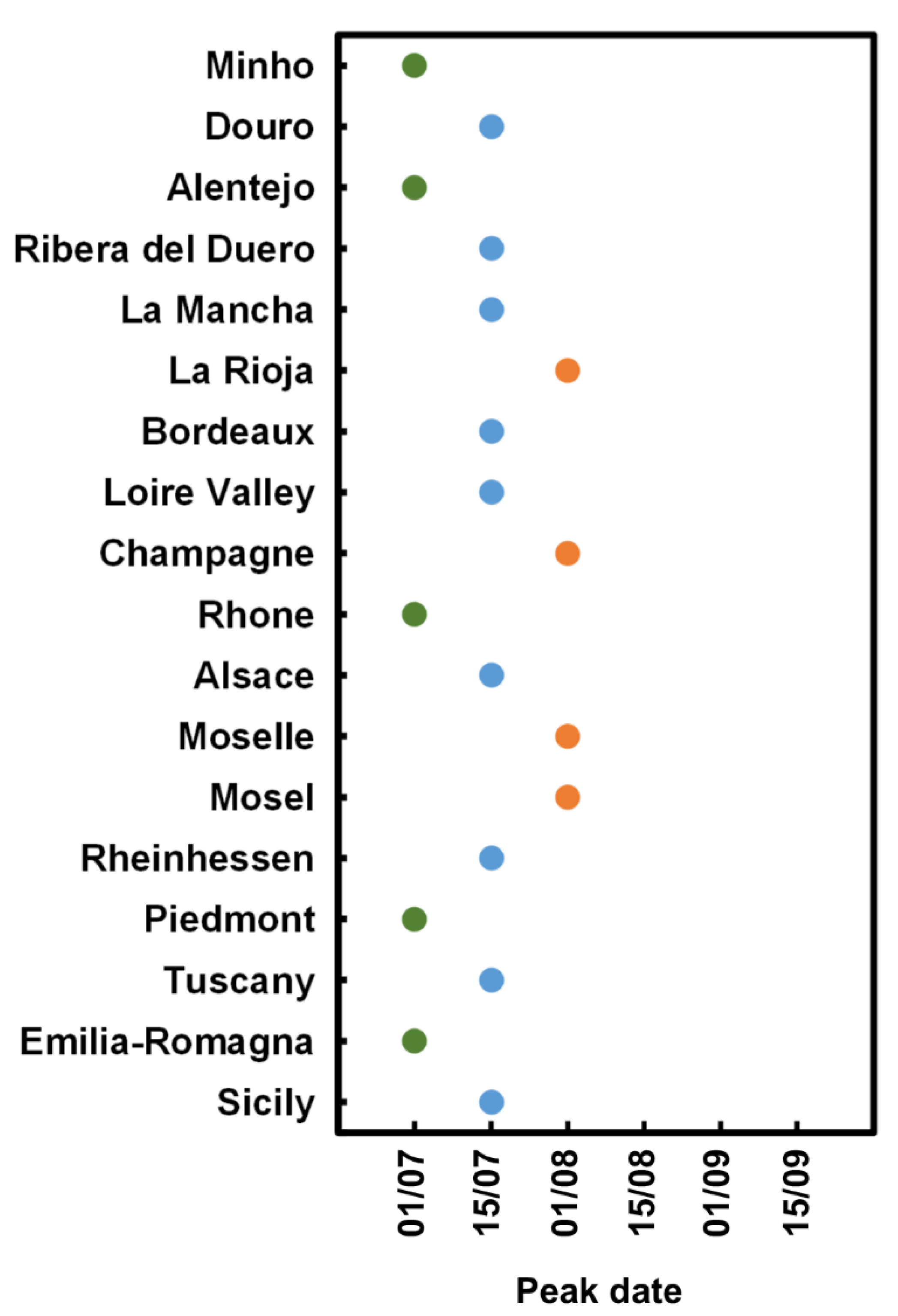
Figure 4 shows a comparison of the peak dates over the 18 selected winemaking regions in Europe. The heatwave peak dates occur before 1 August (inclusively) for all regions. Minho (Portugal), Alentejo (Portugal), Rhone (France), Piedmont and Emilia-Romagna (Italy) reveal stronger heatwaves earlier in the year than other regions. Conversely, La Rioja (Spain), Champagne (France), Moselle (Luxembourg) and Mosel (Germany) will experience stronger impacts when heatwaves occur later (1 August). It should be noted that the regions where the strongest impacts of the heatwaves tend to occur earlier/later are also the regions with the highest/lowest annual mean temperatures (warmer/cooler climates).
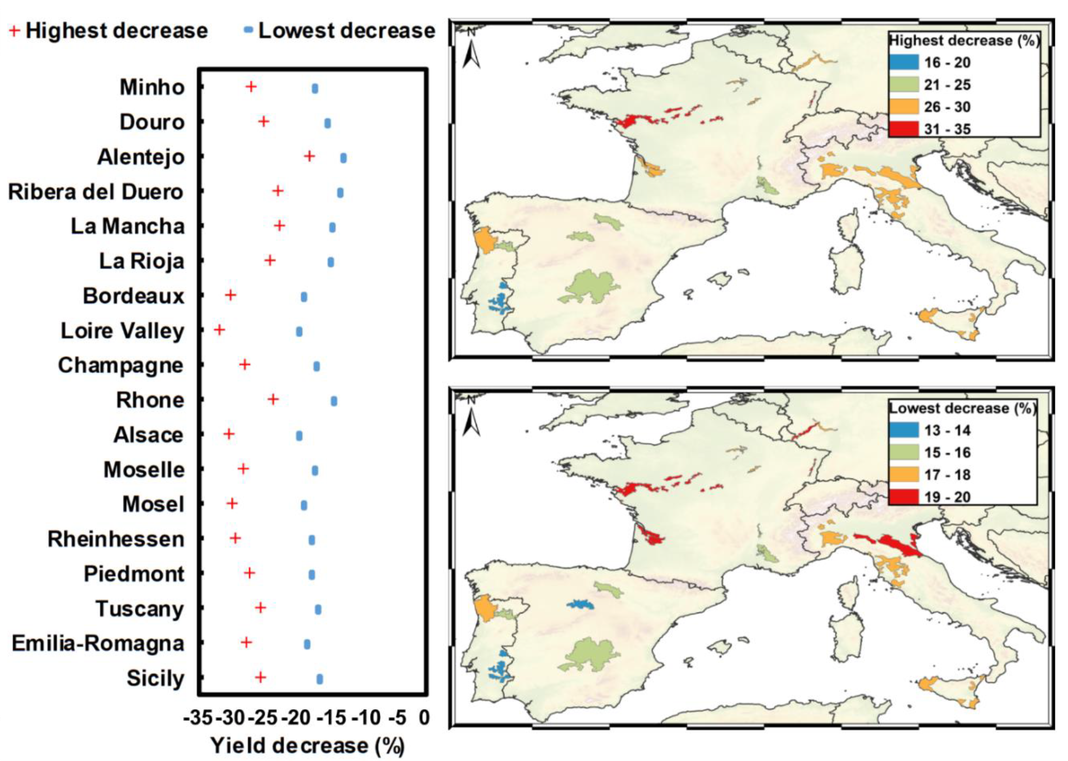
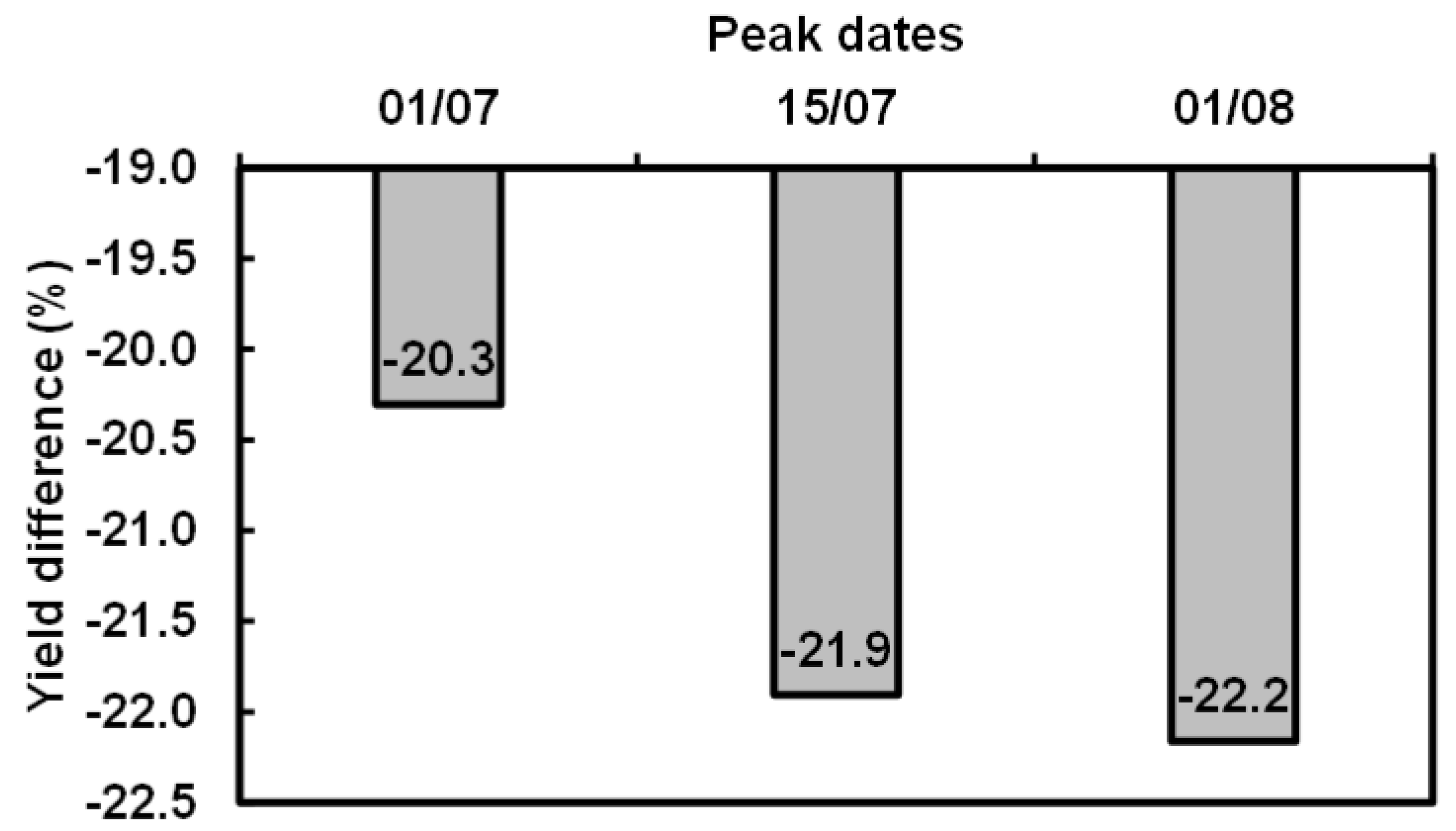
Figure 5 provides a comparison across all regions of the highest and lowest decrease in yields at each peak date. This assessment was based on the heatwave peak date for each region. The results suggest that the most affected regions are the Loire Valley, Alsace and Bordeaux. These regions will undergo yield decreases from −30%/−35% (nine days of heatwaves) to −20% (five days of heatwaves). On the other hand, the least affected region is Alentejo, being the highest decrease of −20%. Figure 6 shows the average yield difference at each peak date for all the regions combined. Results show that the regions where the peak date occurs later (1 August) are more negatively affected than the regions where this peak occurs earlier.
4. Discussion and Conclusions
The results show that heatwaves can have a very strong impact on grapevine yields. These impacts strongly depend on the onset dates and duration of the heatwaves. The highest negative impacts may result in a decrease in the yield by up to −35% in some regions (Figure 5, left panel). The descending-order ranking of the frequency of occurrence of the heatwave peak dates is 15 July, 1 July and 1 August (Figure 4). The results have shown that regions that have their peak date on 1 August will be more negatively impacted than other regions (Figure 6). The impacts of heatwaves before and after these dates resulted in much less yield reduction (Figure 3). Heatwaves in September show a very low impact in many regions. While being true that heatwaves at this specific period may not be very common, this pattern may be modified by climate change.
This reduction in yields is explained by the detrimental effects of extremely high temperatures on grapevine physiology. Several studies have documented these effects [23,48,49,50,51]. As an example, Molitor and Keller [52] showed for the Luxembourgish Moselle region that post-bloom maximum temperatures (especially over the first three weeks after bloom) are negatively correlated with annual yield. This might be explained by the fact that cell division and cell expansion are reduced under heat conditions and, as a result, berries remain smaller [52]. Kliewer [53] demonstrated that temperatures above 32.5 °C between bloom and 12 to 18 days thereafter reduced berry size compared to 25 °C.
The geographical representation of yield reduction hints at a latitudinal gradient in the heatwave impact (Figure 5, right panel). In fact, regions at lower latitudes seem to show slightly lower negative impacts than regions at higher latitudes. This may be partially explained by the fact that vineyards in Southern Europe are most adapted to higher temperatures than regions in Central Europe. Furthermore, productivity in Southern European countries, such as Spain and Portugal, is already typically low [54], when compared to Central Europe, and this productivity difference could partially explain the lower decrease. Under Southern European conditions, the highest yield reductions were observed when a heatwave occurs in July, while this was verified in early August for the northern cooler regions. This might be explained by the later annual phenological cycle under cooler conditions, i.e., it is assumed that the temporal shift in phenology might be the reason for the temporal shift of maximum yield reduction.
Some limitations of the present study can be mentioned. In effect, there are uncertainties inherent to this kind of modelling assessment. The first limitation is tied to the crop model. Although STICS has previously shown a high agreement with observed conditions, the model may not satisfactorily incorporate critical plant processes to assess the full impact of heatwaves. As an example, the model does not include a module to address berry and leaf sunburn, which is a common consequence of heatwaves. Another limitation of the current study is that it does not take into account multiple heatwaves in a single year, i.e., only one heatwave per year was considered. The uncertainty related to the future scenarios should also be mentioned. Increased atmospheric CO2 concentration partially offsets the dryness effects, promoting yield and leaf area index increases in Central/Northern Europe. Moreover, the current study simulations are based on a modification of a single climatic variable (air temperature), whereas several other atmospheric variables can also play a key role during a heatwave, such as air humidity, radiation fluxes, wind and pressure, amongst others. Another aspect is related to the occurrence or not of precipitation in the days before the heatwave, as it may also impact the results.
Furthermore, there is still some uncertainty related to the effect of high temperatures that are not completely understood [30]. As an example, in some studies with reduced stomatal conductance owed to extreme heat exposure, grapevines recovered within a few days [16,19,20]. Furthermore, some varieties are more heat-tolerant than others [55,56], and several acclimatization processes have been identified for extreme temperatures [25,49,57]. In the present study, a single variety (cv. Pinot noir) was used in the modelling approach. Nevertheless, in reality, vineyards in Europe are composed of many rootstocks, cultivars and botanical clones that eventually determine yields, e.g., see [58].
Given these results, and to the projected increase in heatwave occurrence and intensity under future climate conditions, adequate and timely planning of suitable adaptation measures needs to be adopted by the winemaking sector. One of the main adaptation measures is the selection and cultivation of variety-clone-rootstock combinations more resilient to the projected heat and water stress conditions [45]. Additionally, training systems that promote higher water-use efficiency should be envisioned, such as the Gobelet [59]. In general, all measures that promote higher water-use efficiency may be seen as adequate adaptation measures against the negative impact of heatwaves [60,61,62]. The present study may be considered to be a first approach to modelling heatwave impact on grapevines. Although these findings highlight the detrimental impact that heatwaves may bring to the European winegrowers, further research should be envisioned to evaluate and improve these modelling assessments, so as to provide more accurate information regarding the effects of extreme events on viticulture.
5. Conclusions
The present study highlights the negative impacts that heatwaves may have on the main viticultural regions in Europe. This information, is critical for stakeholders and decision-makers within the European winemaking sector, as it allows them to timely plan suitable adaptation measures that may ensure the future sustainability of this important socioeconomic sector.
Author Contributions
All authors have read and agreed to the published version of the manuscript. Conceptualization, H.F.; methodology, H.F.; software, H.F.; validation, H.F., D.M., L.L. and J.A.S.; formal analysis, H.F., D.M., L.L. and J.A.S.; investigation, H.F.; resources, H.F.; data curation, H.F. writing—original draft preparation, H.F.; writing—review and editing, H.F., D.M., L.L. and J.A.S.; visualization, H.F., D.M., L.L. and J.A.S.; supervision, H.F.; project administration, H.F.; funding acquisition, H.F.
Funding
This research was funded by FCT—Portuguese Foundation for Science and Technology contract CEECIND/00447/2017 and Project COA/CAC/0030/2019.
Acknowledgments
Helder Fraga thanks the FCT—Portuguese Foundation for Science and Technology for contract CEECIND/00447/2017. This study was carried out under the CoaClimateRisk FCT Project (COA/CAC/0030/2019). This work was also supported by National Funds by FCT under the project UIDB/04033/2020. We also thank the Clim4Vitis project, “Climate change impact mitigation for European viticulture: knowledge transfer for an integrated approach”, funded by European Union’s Horizon 2020 Research and Innovation Programme, under grant agreement n° 810176.
Conflicts of Interest
The authors declare no conflict of interest.
References
- Kottek, M.; Grieser, J.; Beck, C.; Rudolf, B.; Rubel, F. World map of the Koppen-Geiger climate classification updated. Meteorol. Z. 2006, 15, 259–263. [Google Scholar] [CrossRef]
- Giorgi, F. Climate change hot-spots. Geophys. Res. Lett. 2006, 33. [Google Scholar] [CrossRef]
- Baldocchi, D.; Wong, S. Accumulated winter chill is decreasing in the fruit growing regions of California. Clim. Chang. 2008, 87, S153–S166. [Google Scholar] [CrossRef]
- Luedeling, E.; Girvetz, E.H.; Semenov, M.A.; Brown, P.H. Climate Change Affects Winter Chill for Temperate Fruit and Nut Trees. PLoS ONE 2011, 6, e20155. [Google Scholar] [CrossRef]
- Atkinson, C.J.; Brennan, R.M.; Jones, H.G. Declining chilling and its impact on temperate perennial crops. Environ. Exp. Bot. 2013, 91, 48–62. [Google Scholar] [CrossRef]
- Gladstones, J. Wine, Terroir and Climate Change; Wakefield Press: Adelaide, Australia, 2011. [Google Scholar]
- Keller, M. The Science of Grapevines: Anatomy and Physiology; Elsevier, Inc.: New York, NY, USA, 2010; p. 400. [Google Scholar]
- Coombe, B.G. Influence of temperature on composition and quality of grapes. Acta Hort. 1987, 206, 23–36. [Google Scholar] [CrossRef]
- Schwartz, M.D.; Hanes, J.M. Continental-scale phenology: Warming and chilling. Int. J. Clim. 2010, 30, 1595–1598. [Google Scholar] [CrossRef]
- Winkler, A.J. General Viticulture; University of California Press: Berkeley, CA, USA, 1974. [Google Scholar]
- Bonhomme, R. Review: Bases and limits to using ‘degree.day’ units. Eur. J. Agron. 2000, 13, 1–10. [Google Scholar] [CrossRef]
- Mariani, L.; Parisi, S.; Cola, G.; Failla, O. Climate change in Europe and effects on thermal resources for crops. Int. J. Biometeorol. 2012. [Google Scholar] [CrossRef]
- Wang, E.; Engel, T. Simulation of phenological development of wheat crops. Agric. Syst. 1998, 58, 1–24. [Google Scholar] [CrossRef]
- Yan, W.; Hunt, L.A. An equation for modelling the temperature response of plants using only the cardinal temperatures. Ann. Bot. 1999, 84, 607–614. [Google Scholar] [CrossRef] [Green Version]
- Molitor, D.; Junk, J.; Evers, D.; Hoffmann, L.; Beyer, M. A high resolution cumulative degree day based model to simulate phenological development of grapevine. Am. J. Enol. Vitic. 2014, 65, 72–80. [Google Scholar] [CrossRef]
- Ferrini, F.; Mattii, G.B.; Nicese, F.P. Effect of Temperature on Key Physiological Responses of Grapevine Leaf. Am. J. Enol. Vitic. 1995, 46, 375. [Google Scholar]
- Moutinho-Pereira, J.M.; Correia, C.M.; Goncalves, B.M.; Bacelar, E.A.; Torres-Pereira, J.M. Leaf gas exchange and water relations of grapevines grown in three different conditions. Photosynthetica 2004, 42, 81–86. [Google Scholar] [CrossRef]
- Berry, J.; Bjorkman, O. Photosynthetic Response and Adaptation to Temperature in Higher-Plants. Annu. Rev. Plant Physiol. Plant Mol. Biol. 1980, 31, 491–543. [Google Scholar] [CrossRef]
- Matsui, S.; Ryugo, K.; Kliewer, W.M. Lowered Berry Quality Due to Heat Stress at the Early Ripening Stage of Berry Growth in a Seeded Grapevine, Vitis vinifera L.; Research Bulletin of the Faculty of Agriculture-Gifu University: Gifu, Japan, 1991. [Google Scholar]
- Sepúlveda, G.; Kliewer, W.M. Stomatal Response of Three Grapevine Cultivars (Vitis vinifera L.) to High Temperature. Am. J. Enol. Vitic. 1986, 37, 44. [Google Scholar]
- Kliewer, W.M. Influence of Temperature, Solar Radiation and Nitrogen on Coloration and Composition of Emperor Grapes. Am. J. Enol. Vitic. 1977, 28, 96. [Google Scholar]
- Schultz, H.R. Extension of a Farquhar model for limitations of leaf photosynthesis induced by light environment, phenology and leaf age in grapevines (Vitis vinifera L. cvv. White Riesling and Zinfandel). Funct. Plant Biol. 2003, 30, 673–687. [Google Scholar] [CrossRef]
- Greer, D.H.; Weston, C. Heat stress affects flowering, berry growth, sugar accumulation and photosynthesis of Vitis vinifera cv. Semillon grapevines grown in a controlled environment. Funct. Plant Biol. 2010, 37, 206–214. [Google Scholar] [CrossRef]
- Ingvordsen, C.H.; Lyngkjaer, M.F.; Peltonen-Sainio, P.; Mikkelsen, T.N.; Stockmarr, A.; Jorgensen, R.B. How a 10-day heatwave impacts barley grain yield when superimposed onto future levels of temperature and CO2 as single and combined factors. Agric. Ecosyst. Environ. 2018, 259, 45–52. [Google Scholar] [CrossRef] [Green Version]
- Grace, W.J.; Sadras, V.O.; Hayman, P.T. Modelling heatwaves in viticultural regions of southeastern Australia. Aust. Meteorol. Oceanogr. J. 2009, 58, 249–262. [Google Scholar] [CrossRef]
- Menzel, A. A 500 year pheno-climatological view on the 2003 heatwave in Europe assessed by grape harvest dates. Meteorol. Z. 2005, 14, 75–77. [Google Scholar] [CrossRef]
- Beniston, M. The 2003 heat wave in Europe: A shape of things to come? An analysis based on Swiss climatological data and model simulations. Geophys. Res. Lett. 2004, 31. [Google Scholar] [CrossRef] [Green Version]
- Costa, R.; Fraga, H.; Fonseca, A.; de Cortazar-Atauri, I.G.; Val, M.C.; Carlos, C.; Reis, S.; Santos, J.A. Grapevine Phenology of cv. Touriga Franca and Touriga Nacional in the Douro Wine Region: Modelling and Climate Change Projections. Agronomy 2019, 9, 210. [Google Scholar] [CrossRef] [Green Version]
- Moriondo, M.; Ferrise, R.; Trombi, G.; Brilli, L.; Dibari, C.; Bindi, M. Modelling olive trees and grapevines in a changing climate. Environ. Model. Softw. 2015, 72, 387–401. [Google Scholar] [CrossRef]
- Leolini, L.; Bregaglio, S.; Moriondo, M.; Ramos, M.C.; Bindi, M.; Ginaldi, F. A model library to simulate grapevine growth and development: Software implementation, sensitivity analysis and field level application. Eur. J. Agron. 2018, 99, 92–105. [Google Scholar] [CrossRef]
- Brisson, N.; Launay, M.; Mary, B.; Beaudoin, N. Conceptual Basis, Formalisations and Parameterization of the STICS Crop Model; Editions Quae: Versailles, France, 2008; p. 297. [Google Scholar]
- García de Cortazar-Atauri, I. Adaptation du Modèle STICS à la Vigne (Vitis vinifera L.). Utilisation Dans le Cadre d’une étude d’impact du Changement Climatique à l’échelle de la France. Ph.D. Thesis, Ecole Nationale Supérieure Agronomique, Montpellier, France, 2006. [Google Scholar]
- Fraga, H.; Costa, R.; Moutinho-Pereira, J.; Correia, C.M.; Dinis, L.-T.; Gonçalves, I.; Silvestre, J.; Eiras-Dias, J.; Malheiro, A.C.; Santos, J.A. Modeling Phenology, Water Status, and Yield Components of Three Portuguese Grapevines Using the STICS Crop Model. Am. J. Enol. Vitic. 2015, 66, 482–491. [Google Scholar] [CrossRef]
- Valdes-Gomez, H.; Celette, F.; García de Cortazar-Atauri, I.; Jara-Rojas, F.; Ortega-Farias, S.; Gary, C. Modelling Soil Water Content and Grapevine Growth and Development with the Stics Crop-Soil Model under Two Different Water Management Strategies. J. Int. Des. Sci. De La Vigne Et Du Vin 2009, 43, 13–28. [Google Scholar] [CrossRef] [Green Version]
- Fraga, H.; García de Cortázar Atauri, I.; Malheiro, A.C.; Santos, J.A. Modelling climate change impacts on viticultural yield, phenology and stress conditions in Europe. Glob. Chang. Biol. 2016, 22, 3774–3788. [Google Scholar] [CrossRef]
- Fraga, H.; Santos, J.A.; Moutinho-Pereira, J.; Carlos, C.; Silvestre, J.; Eiras-Dias, J.; Mota, T.; Malheiro, A.C. Statistical modelling of grapevine phenology in Portuguese wine regions: Observed trends and climate change projections. J. Agric. Sci. 2015, FirstView, 1–17. [Google Scholar] [CrossRef] [Green Version]
- Fraga, H.; Santos, J.A. Vineyard mulching as a climate change adaptation measure: Future simulations for Alentejo, Portugal. Agric. Syst. 2018, 164, 107–115. [Google Scholar] [CrossRef]
- Fraga, H.; García de Cortázar Atauri, I.; Santos, J.A. Viticultural irrigation demands under climate change scenarios in Portugal. Agric. Water Manag. 2018, 196, 66–74. [Google Scholar] [CrossRef]
- García de Cortazar-Atauri, I.; Brisson, N.; Gaudillere, J.P. Performance of several models for predicting budburst date of grapevine (Vitis vinifera L.). Int. J. Biometeorol. 2009, 53, 317–326. [Google Scholar] [CrossRef]
- García de Cortazar-Atauri, I.; Brisson, N.; Ollat, N.; Jacquet, O.; Payan, J.C. Asynchronous dynamics of grapevine (Vitis vinifera) maturation: Experimental study for a modelling approach. J. Int. Des Sci. De La Vigne Et Du Vin 2009, 43, 83–97. [Google Scholar] [CrossRef]
- Cornes, R.C.; van der Schrier, G.; van den Besselaar, E.J.M.; Jones, P.D. An Ensemble Version of the E-OBS Temperature and Precipitation Data Sets. J. Geophys. Res. Atmos. 2018, 123, 9391–9409. [Google Scholar] [CrossRef] [Green Version]
- C3S. ERA5: Fifth Generation of ECMWF Atmospheric Reanalysis of the Global Climate. Copernicus Climate Change Service Climate Data Store (CDS), 2017. Available online: https://climate.copernicus.eu/climate-data-store (accessed on 1 February 2020).
- FAO/IIASA/ISRIC/ISSCAS/JRC. Harmonized World Soil Database (version 1.2); FAO: Rome, Italy; IIASA: Laxenburg, Austria, 2012. [Google Scholar]
- Bouma, J. Using Soil Survey Data for Quantitative Land Evaluation. In Advances in Soil Science; Stewart, B.A., Ed.; Springer: New York, NY, USA, 1989; Volume 9, pp. 177–213. [Google Scholar]
- Jones, G.V. Climate and Terroir: Impacts of Climate Variability and Change on Wine in Fine Wine and Terroir—The Geoscience Perspective; Macqueen, R.W., Meinert, L.D., Eds.; Geoscience Canada, Geological Association of Canada: St. John’s, NL, Canada, 2006. [Google Scholar]
- Anderson, K.; Aryal, N.R. Which Winegrape Varieties are Grown Where? A Global Empirical Picture; University of Adelaide Press: Adelaide, Australia, 2013; 700p. [Google Scholar]
- Jackson, R.S. Wine Science: Principles and Applications; Elsevier Science: Amsterdam, The Netherlands, 2008; 776p. [Google Scholar]
- White, M.A.; Diffenbaugh, N.S.; Jones, G.V.; Pal, J.S.; Giorgi, F. Extreme heat reduces and shifts United States premium wine production in the 21st century. Proc. Natl. Acad. Sci. USA 2006, 103, 11217–11222. [Google Scholar] [CrossRef] [Green Version]
- Carvalho, L.C.; Coito, J.L.; Colaco, S.; Sangiogo, M.; Amancio, S. Heat stress in grapevine: The pros and cons of acclimation. Plant Cell Environ. 2015, 38, 777–789. [Google Scholar] [CrossRef]
- Greer, D.H.; Weedon, M.M.; Weston, C. Reductions in biomass accumulation, photosynthesis in situ and net carbon balance are the costs of protecting Vitis vinifera ‘Semillon’ grapevines from heat stress with shade covering. Aob Plants 2011, 2011, plr023. [Google Scholar] [CrossRef]
- Webb, L.; Watt, A.; Hill, T.; Whiting, J.; Wigg, F.; Dunn, G.; Needs, S.; Barlow, E.W.R. Extreme Heat: Managing Grapevine Response. Documenting Regional and Inter-Regional Variation of Viticultural Impact and Management Input Relating to the 2009 Heatwave in South-Eastern Australia. GWRDC and University of Melbourne: Melbourne; University of Melbourne: Melbourne, Australia, 2009. [Google Scholar]
- Molitor, D.; Keller, M. Yield of Müller-Thurgau and Riesling grapevines is altered by meteorological conditions in the current and the previous growing seasons. OENO One 2016, 50, 245–258. [Google Scholar]
- Kliewer, W.M. Effect of High-Temperatures during Bloom-Set Period on Fruit-Set, Ovule Fertility, and Berry Growth of Several Grape Cultivars. Am. J. Enol. Vitic. 1977, 28, 215–222. [Google Scholar]
- OIV. 2019 Statistical Report on World Vitiviniculture; International Organisation of Vine and Wine: Paris, France, 2019. [Google Scholar]
- Schaffer, B.; Andersen, P.C. Handbook of Environmental Physiology of Fruit Crops. Volume 1. Temperature Crops; CRC Press: Boca Raton, FL, USA, 1994; 358p. [Google Scholar]
- Moutinho-Pereira, J.; Magalhães, N.; Gonçalves, B.; Bacelar, E.; Brito, M.; Correia, C. Gas exchange and water relations of three Vitis vinifera L. cultivars growing under Mediterranean climate. Photosynthetica 2007, 45, 202–207. [Google Scholar] [CrossRef]
- Wang, L.J.; Li, S.H. Thermotolerance and related antioxidant enzyme activities induced by heat acclimation and salicylic acid in grape (Vitis vinifera L.) leaves. Plant Growth Regul. 2006, 48, 137–144. [Google Scholar] [CrossRef]
- Renouf, V.; Tregoat, O.; Roby, J.P.; Van Leeuwen, C. Soils, Rootstocks and Grapevine Varieties in Prestigious Bordeaux Vineyards and Their Impact on Yield and Quality. J. Int. Des Sci. De La Vigne Et Du Vin 2010, 44, 127–134. [Google Scholar] [CrossRef]
- Van Leeuwen, C.; Darriet, P. The Impact of Climate Change on Viticulture and Wine Quality. J. Wine Econ. 2016, 11, 150–167. [Google Scholar] [CrossRef] [Green Version]
- Chaves, M.M.; Santos, T.P.; Souza, C.R.; Ortuno, M.F.; Rodrigues, M.L.; Lopes, C.M.; Maroco, J.P.; Pereira, J.S. Deficit irrigation in grapevine improves water-use efficiency while controlling vigour and production quality. Ann. Appl. Biol. 2007, 150, 237–252. [Google Scholar] [CrossRef]
- Fraga, H.; Atauri, I.G.D.; Malheiro, A.C.; Moutinho-Pereira, J.; Santos, J.A. Viticulture in Portugal: A review of recent trends and climate change projections. OENO One 2017, 51, 61–69. [Google Scholar] [CrossRef] [Green Version]
- Fraga, H.; Santos, J.A. Daily prediction of seasonal grapevine production in the Douro wine region based on favourable meteorological conditions. Aust. J. Grape Wine Res. 2017, 23, 296–304. [Google Scholar] [CrossRef]
Figure 1.
Selected wine regions in Europe (18), highlighted by a black line contour, and their corresponding designations. Other wine regions are also outlined, with different color shadings for different countries.
Figure 1.
Selected wine regions in Europe (18), highlighted by a black line contour, and their corresponding designations. Other wine regions are also outlined, with different color shadings for different countries.

Figure 2.
Illustrative representation of the synthetic heatwave disturbances/pulses during a calendar year, outlining their onset (dates within color bars), duration (color bar width) and intensity (color bar top). The observed temperature time series are represented by the background shaded graph, while the synthetic temperature time series of the heatwave disturbances are indicated at the top of each color bar.

Figure 3.
Yield relative difference (in %) between normal years and years with heatwaves, with a duration from five to nine days, in (a) Minho, (b) Douro, (c) Alentejo, (d) Ribera del Duero, (e) La Mancha, (f) La Rioja, (g) Bordeaux, (h) Loire Valley, (i) Champagne, (j) Rhone, (k) Alsace, (l) Moselle, (m) Mosel, (n) Rheinhessen, (o) Piedmont, (p) Tuscany, (q) Emilia-Romagna and (r) Sicily, depending on to the date of onset of the heatwave.

Figure 4.
Comparison of the heatwave peak dates over the 18 selected winemaking regions in Europe. Different peak dates are represented by different colors.
Figure 4.
Comparison of the heatwave peak dates over the 18 selected winemaking regions in Europe. Different peak dates are represented by different colors.

Figure 5.
Left panel: highest and lowest yield decrease due to heatwaves for each winemaking region at the peak date. Right panel: geographical representation of the highest and lowest decrease in yields over Europe at the peak date.
Figure 5.
Left panel: highest and lowest yield decrease due to heatwaves for each winemaking region at the peak date. Right panel: geographical representation of the highest and lowest decrease in yields over Europe at the peak date.

Figure 6.
Average relative yield differences (%) for all the regions at each peak date.


Table 1.
Targeted winemaking regions (18 in total), with country and region designation, along with their centroid longitude and latitude, and area-means of annual mean temperature (T) and precipitation sum (P), calculated from the E-OBS dataset, version 19.0e, over the baseline period of 1986–2015. The three highest and lowest values are highlighted in bold.
| COUNTRY | REGION | LON (°) | LAT (°) | T (°C) | P (mm) |
|---|---|---|---|---|---|
| France | Alsace | 7.38 | 48.20 | 10.6 | 605 |
| Bordeaux | 0.55 | 44.50 | 13.2 | 807 | |
| Champagne | 4.00 | 49.16 | 10.5 | 664 | |
| Loire Valley | 0.13 | 47.12 | 12.3 | 684 | |
| Rhone | 4.83 | 44.06 | 14.7 | 733 | |
| Germany | Mosel | 6.87 | 49.28 | 10.4 | 766 |
| Rheinhessen | 8.13 | 49.92 | 10.6 | 579 | |
| Italy | Emilia-Romagna | 10.93 | 44.50 | 13.1 | 840 |
| Piedmont | 8.67 | 44.66 | 13.3 | 988 | |
| Sicily | 13.99 | 37.64 | 15.9 | 482 | |
| Tuscany | 11.77 | 43.08 | 13.6 | 723 | |
| Luxembourg | Moselle | 6.35 | 49.55 | 10.3 | 743 |
| Portugal | Alentejo | −7.56 | 38.38 | 17.2 | 562 |
| Douro | −7.55 | 41.17 | 13.3 | 830 | |
| Minho | −8.41 | 41.82 | 14.1 | 956 | |
| Spain | La Mancha | −2.69 | 39.65 | 14.2 | 455 |
| La Rioja | −2.40 | 41.57 | 11.5 | 523 | |
| Ribera del Duero | −4.36 | 41.63 | 12.3 | 423 |
© 2020 by the authors. Licensee MDPI, Basel, Switzerland. This article is an open access article distributed under the terms and conditions of the Creative Commons Attribution (CC BY) license (http://creativecommons.org/licenses/by/4.0/).
Share and Cite
MDPI and ACS Style
Fraga, H.; Molitor, D.; Leolini, L.; Santos, J.A. What Is the Impact of Heatwaves on European Viticulture? A Modelling Assessment. Appl. Sci. 2020, 10, 3030. https://0-doi-org.brum.beds.ac.uk/10.3390/app10093030
AMA Style
Fraga H, Molitor D, Leolini L, Santos JA. What Is the Impact of Heatwaves on European Viticulture? A Modelling Assessment. Applied Sciences. 2020; 10(9):3030. https://0-doi-org.brum.beds.ac.uk/10.3390/app10093030
Chicago/Turabian StyleFraga, Helder, Daniel Molitor, Luisa Leolini, and João A. Santos. 2020. "What Is the Impact of Heatwaves on European Viticulture? A Modelling Assessment" Applied Sciences 10, no. 9: 3030. https://0-doi-org.brum.beds.ac.uk/10.3390/app10093030
Note that from the first issue of 2016, this journal uses article numbers instead of page numbers. See further details here.