Article

Phenological Model Intercomparison for Estimating Grapevine Budbreak Date (Vitis vinifera L.) in Europe

1
Department of Agriculture, Food, Environment and Forestry, DAGRI, University of Florence, UNIFI, 50144 Florence, Italy
2
Centre for the Research and Technology of Agro-Environmental Sciences, CITAB, Universidade de Trás-os-Montes e Alto Douro, UTAD, 5000-801 Vila Real, Portugal
3
Potsdam Institute for Climate Impact Research, PIK, 14473 Potsdam, Germany
4
Luxembourg Institute of Science and Technology, LIST, 4422 Luxembourg, Luxembourg
5
Tropical Plant Production and Agricultural Systems Modelling—TROPAGS, University of Göttingen, 37077 Göttingen, Germany
6
EGFV, Bordeaux Sciences Agro, INRAE, University of Bordeaux, ISVV, F-33882 Villenave d’Ornon, France
7
Instituto Nacional de Investigação Agrária e Veterinária, INIAV, Estação Vitivinícola Nacional, Quinta da Almoínha, 2565-191 Dois Portos, Portugal
8
Institute of Bioeconomy, National Research Council, CNR-IBE, 50019 Florence, Italy
*
Author to whom correspondence should be addressed.
Submission received: 16 April 2020 / Revised: 20 May 2020 / Accepted: 22 May 2020 / Published: 29 May 2020

Abstract

:
Budbreak date in grapevine is strictly dependent on temperature, and the correct simulation of its occurrence is of great interest since it may have major consequences on the final yield and quality. In this study, we evaluated the reliability for budbreak simulation of two modeling approaches, the chilling-forcing (CF), which describes the entire dormancy period (endo- and eco-dormancy) and the forcing approach (F), which only describes the eco-dormancy. For this, we selected six phenological models that apply CF and F in different ways, which were tested on budbreak simulation of eight grapevine varieties cultivated at different latitudes in Europe. Although none of the compared models showed a clear supremacy over the others, models based on CF showed a generally higher estimation accuracy than F where fixed starting dates were adopted. In the latter models, the accurate simulation of budbreak was dependent on the selection of the starting date for forcing accumulation that changes according to the latitude, whereas CF models were independent. Indeed, distinct thermal requirements were found for the grapevine varieties cultivated in Northern and Southern Europe. This implies the need to improve modeling of the dormancy period to avoid under- or over-estimations of budbreak date under different environmental conditions.

1. Introduction

Grapevine phenological phases have a profound influence on the final grape and wine quality [1,2,3]. In particular, changes in the current climate conditions are strongly affecting the occurrence of the developmental stages and length of the grapevine growing cycle in the most renowned wine areas [4,5].
Several authors have reported the increasing temperature trend across the most traditional wine areas of the Mediterranean basin during the last decades. For example, Tomasi et al. [6] showed a 2.3 °C-temperature increase over the grape growing season in Veneto region (Italy) during the period 1964-2009, while van Leeuwen et al. [7] evidenced a 2.0 °C increase from 1951 to 2016 in the Bordeaux wine production area. Moreover, Ramos et al. [8] observed an overall warming from 1.0 to 2.2 °C during the grape growing season in north-eastern Spain. These changes are expected to greatly influence grapevine varietal suitability across the European region [9,10,11,12].
Since grapevine phenology is mainly temperature-driven [4], the current warming is affecting the phenological stages and shifting the annual growing cycle [13,14,15,16]. Among the most important developmental phases, budbreak represents the starting point of vegetative growth. A temperature increase can have a dual effect on this phase (anticipating or delaying its occurrence), with strong consequences on the following reproductive stages. Indeed, a shift in budbreak may determine poor shoot growth together with fewer clusters and an inhomogeneous grape development [17,18].
Under increasing temperature, a delay in budbreak phase can be determined by insufficient chilling during the dormancy period [19]. Indeed, the bud vegetative growth is limited by a first sub-period induced by physiological conditions (endo-dormancy), and then by a second sub-period in which bud opening is affected by the environmental conditions (eco-dormancy [17,20]). In this context, some studies showed that dormancy release is regulated by bud exposure period to temperatures between 0 to 10 °C [19,21], until fulfilment of the chilling requirement, and a subsequent period of temperatures (from 0 to 25 °C), until the reaching of the forcing requirement [22].
Budbreak occurrence being strongly influenced by the dormancy period, several studies attempted the implementation of phenological models for improving the prediction of this developmental stage [23,24,25,26,27,28]. Phenological models can be classified in two main categories: forcing and chilling-forcing models. Forcing models are simply based on the forcing unit accumulation, starting, in general, from a fixed date in the year. These models only focus on the description of the eco-dormancy period assuming that the chilling unit accumulation requirement was previously fulfilled and the endo-dormancy period had concluded. Instead, chilling-forcing models can explain both the endo- and eco-dormancy periods by taking into consideration the chilling unit and the forcing accumulation with respect to specific temperature thresholds [24,29,30].
Hence, the selection of one of these two categories for an accurate budbreak simulation often gave rise to a wide debate [29,30]. Chilling-forcing models can take into account the influences of temperature on the entire dormancy period, evidencing not only the shortening effect of warmer temperatures during eco-dormancy but also a possible delay of budbreak caused by a failed chilling requirement [13,31]. However, the limited improvement in the performances of these models and the easier implementation provided by forcing models, focus on the issue about the most suitable modeling approach for budbreak estimation. In modeling studies, the choice of phenological model plays an important role in the use of crop simulation models and in determining potential risk of late spring frost events. In crop simulation models, phenology defines the plant growing cycle with important consequences on future biomass partitioning [32]. In this context, an accurate estimation of budbreak stage may avoid randomly selecting a starting point for vegetative biomass accumulation and over- or under-detection of late spring frost events under different climate scenarios [31,33].
Thus, the phenological intercomparison may be useful to highlight the performances of different models in simulating budbreak [29,30]. In order to take into account the influences of the grapevine precocity cycle and the effects of environmental conditions on budbreak estimation, model intercomparison experiments should consider multiple grapevine varieties and study sites. Indeed, grapevine varieties are characterized by various thermal requirements and focusing on a specific variety does not allow the range of different physiological responses derived from the impact of temperature on dormancy period to be highlighted [30]. In addition, the use of a single date as a starting point for the chilling and forcing accumulation [29] does not allow the influence of temperature on the beginning of endo- or eco-dormancy periods to be appreciated, especially when the model intercomparison is performed with phenological data of grapevine varieties collected in different environments.
The objective of this study is to evaluate the performances of six phenological models (BRIN tested using hourly and daily temperature) at reproducing the budbreak date of eight grapevine varieties collected at different latitudes in Europe. In order to consider the influences of temperature during the dormancy period on model representations, two starting dates were set during chilling-forcing and forcing models’ simulation, respectively. The analysis of budbreak date estimation is thus addressed to obtain responses of grapevine varieties’ behavior under different environments.

2. Materials and Methods
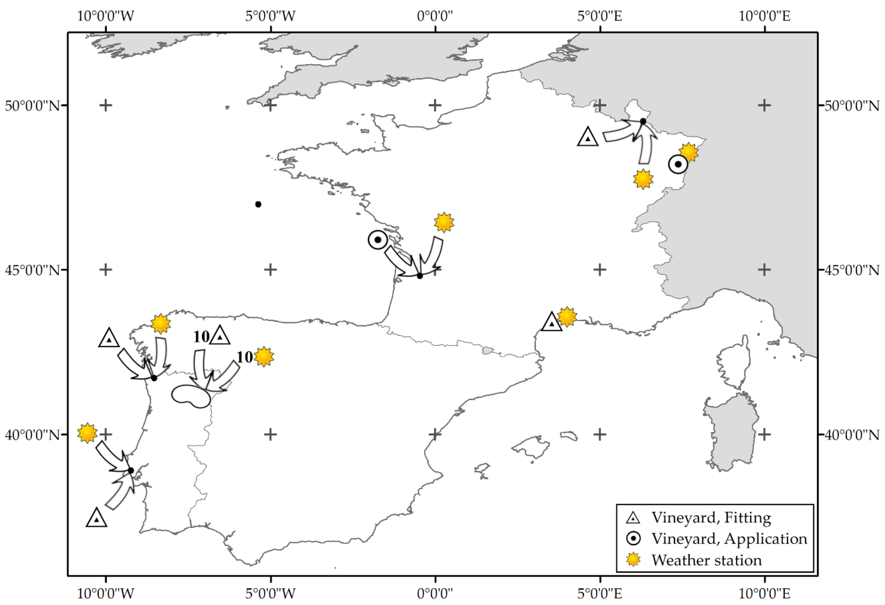
2.1. Observations

The phenological data were collected from 15 experimental vineyards in three European countries (France, Luxembourg and Portugal, see Figure 1 and Table 1). The weather data (i.e., daily maximum and minimum air temperature, °C) were freely available from weather services. More specifically, for France, the land-based daily weather data were collected by the National Centers for Environmental Information and then archived at NOAA (https://www.ncdc.noaa.gov/ [34]) and from a weather station near the VitAdapt project [35]. Hourly temperatures, rainfall, wind speed and reference evapotranspiration were recorded and stored in Climatik, a database managed by INRA, US 1116 Agroclim research station, 84914 Avignon, France (https://intranet.inra.fr/climatik_v2; limited access). For Luxembourg, the weather data were collected by the Administration des Services Techniques de l’Agriculture at the Institut Viti-Vinicole (https://agriculture.public.lu/) while the weather data for Portugal derived from the Instituto Nacional de Investigação Agrária e Veterinária (INIAV http://www.iniav.pt/) and the Associação para o Desenvolvimento da Viticultura Duriense (ADVID https://www.advid.pt/). The weather data were obtained from the closest and more representative stations for the vineyard weather conditions (Figure 1 and Table 1).
The phenological data were collected for eight grapevine varieties (Cabernet Sauvignon, Chardonnay, Gewürztraminer, Grenache, Pinot Gris, Riesling, Touriga Franca and Touriga Nacional). For France, these data were retrieved from PERPHECLIM platform (https://www6.inrae.fr/projet-accaf-perpheclim_eng/The-PERPHECLIM-project [36]) and VitAdapt project [35]. For Luxembourg, the data were obtained from the Administration des Services Techniques de l’Agriculture at the Institut Viti-Vinicole. Finally, the data for the Lisbon wine region (Portugal) were obtained from the national ampelographic collection at the INIAV, located in Dois Portos. The data for the Douro wine region were collected by the associates from ADVID. Most of these grapevine varieties are for high-quality wine production derived from the world’s benchmark regions and can be grouped on the basis of average growing season temperatures and ripening potential [37]. The phenological observations were collected by different research institutions and farmers at budbreak date which typically corresponded to BBCH 09 [38], except for Cabernet Sauvignon, Touriga Franca and Touriga Nacional collected in France (Bordeaux site; BBCH 07). We assumed that the distance between BBCH 07 and 09 is covered in 2 days as reported in [27].

2.2. Phenological Models

In total, we tested 6 models for estimating the budbreak date, divided into forcing (F) and chilling-forcing (CF) models. We used Growing Degree Days (GDD; [39]), WANG [40] and UNIFORC [24] for F models and BRIN [29] (Hourly and Daily approach), UNICHILL and UNIFIED [24] for CF models.

2.2.1. GDD

The GDD model [39] is an F model that describes the eco-dormancy period based on accumulation of the daily average temperature ( T a v g ; °C) above a specific threshold ( T b ; °C). The GDD accumulation ( F o r c G D D ) starts at a fixed date of the year ( t 0 ) and is accumulated until the GDD requirement is satisfied at budbreak date ( B u d ; Equation (1)).
F o r c G D D = t 0 B u d ( T a v g T b ) ,

2.2.2. WANG

The WANG model [40] is a temperature response function used, in this study, to describe the eco-dormancy period from a fixed date of the year ( t 0 ) and not to calculate the chilling unit accumulation as reported for other similar functions [30]. The temperature function ( F o r c W A N G ) allows the phenological development of grapevine to be evaluated using a non-linear approach based on three cardinal temperatures: T o p t (optimum temperature, °C), T max (maximum temperature, °C) and T min (minimum temperature, °C; Equations (2a) and (2b)).
F o r c W A N G = t 0 B u d M a x [ ( 2 ( T a v g T min ) α ( T o p t T min ) α ( T a v g T min ) 2 α ( T o p t T min ) 2 α ) , 0 ] ,
with   α = ln ( 2 ) ln ( T max T min T o p t T min ) ,
where T a v g is the daily average temperature (°C) and B u d is the budbreak date.

2.2.3. UNIFORC

The UNIFORC model [24] is an F model based on a sigmoid curve for calculating the forcing unit accumulation ( F o r c U N I F O R C ) from a fixed day of the year ( t 0 ) until budbreak occurrence ( B u d ; Equation (3)):
F o r c U N I F O R C = t 0 B u d 1 1 + e d ( T a v g e ) ,
where T a v g is daily average temperature (°C), while d and e ( d < 0 and e > 0) are empirical parameters of the function.

2.2.4. BRIN

The BRIN model [29] is a CF model based on the Bidabe’s Cold Action Model [41,42] in which the endo-dormancy period is evaluated through the accumulation of chilling units ( C h i l l B R I N ; Equation (4)). The eco-dormancy period is based on forcing unit accumulation ( F o r c B R I N ) calculated with the Richardson equation [23]. The F o r c B R I N is computed using both a daily (Equation (5)) and hourly (Equations (6a) and (6b)) temperature accumulation approach.
C h i l l B R I N = t 0 C e n d o ( Q 10 c T x ( n ) 10 + Q 10 c T n ( n ) 10 ) ,
F o r c B R I N D a i l y = C e n d o B u d R i c h a r d s o n D a i l y ( n ) ,
F o r c B R I N H o u r l y = C e n d o B u d R i c h a r d s o n H o u r l y ( n )
R i c h a r d s o n = M a x ( M i n ( T a v g T l , T h T l ) , 0 ) ,
where t 0 is the simulation starting date, T a v g is daily average temperature (°C), C e n d o is the date at which the chilling requirement is satisfied, B u d is budbreak date, Q 10 c is the geometric progression rate of the thermal dormancy response, T n and T x are daily minimum and maximum temperatures (°C), respectively. R i c h a r d s o n D a i l y and R i c h a r d s o n H o u r l y are daily and hourly Richardson equations used for representing the eco-dormancy period [29]. The Richardson equations are limited by two cardinal temperatures: a lower ( T l , °C) and an upper limit temperature ( T h , °C).

2.2.5. UNICHILL

The UNICHILL model [24] is a CF two-phase sequential model constituted by two functions describing chilling accumulation ( C h i l l U N I C H I L L ) during endo-dormancy (Equation (7)) and forcing unit accumulation ( F o r c U N I C H I L L ) during eco-dormancy period (Equation (8)). After chilling requirement is satisfied at a specific date ( C e n d o ), the forcing units start accumulating until the forcing requirement is reached, leading to the occurrence of the budbreak phase ( B u d ). The two functions are defined as followed:
C h i l l U N I C H I L L = t 0 C e n d o 1 1 + e a ( T a v g c ) 2 + b ( T a v g c ) ,
F o r c U N I C H I L L = C e n d o B u d 1 1 + e d ( T a v g e ) ,
where t 0 is the simulation starting date, T a v g is daily average temperature (°C) and a , b , c , d and e are empirical parameters of the function.

2.2.6. UNIFIED

The UNIFIED model [24] is a CF overlapping model based on the same equations for chilling and forcing unit accumulation used in the UNICHILL model. However, UNIFIED model includes the effect of chilling units on forcing accumulation through implementation of the exponential decrease curve (Equation (9)) in which F o r c R e q U N I F I E D (Fcrit) is the critical amount of forcing and C h i l l U N I F I E D is the total amount of chilling at day t d . The budbreak date is estimated when both chilling and forcing requirements are satisfied:
F o r c R e q U N I F I E D = w e z C h i l l U N I F I E D ( t d ) ,
where w and z are empirical parameters of the function.

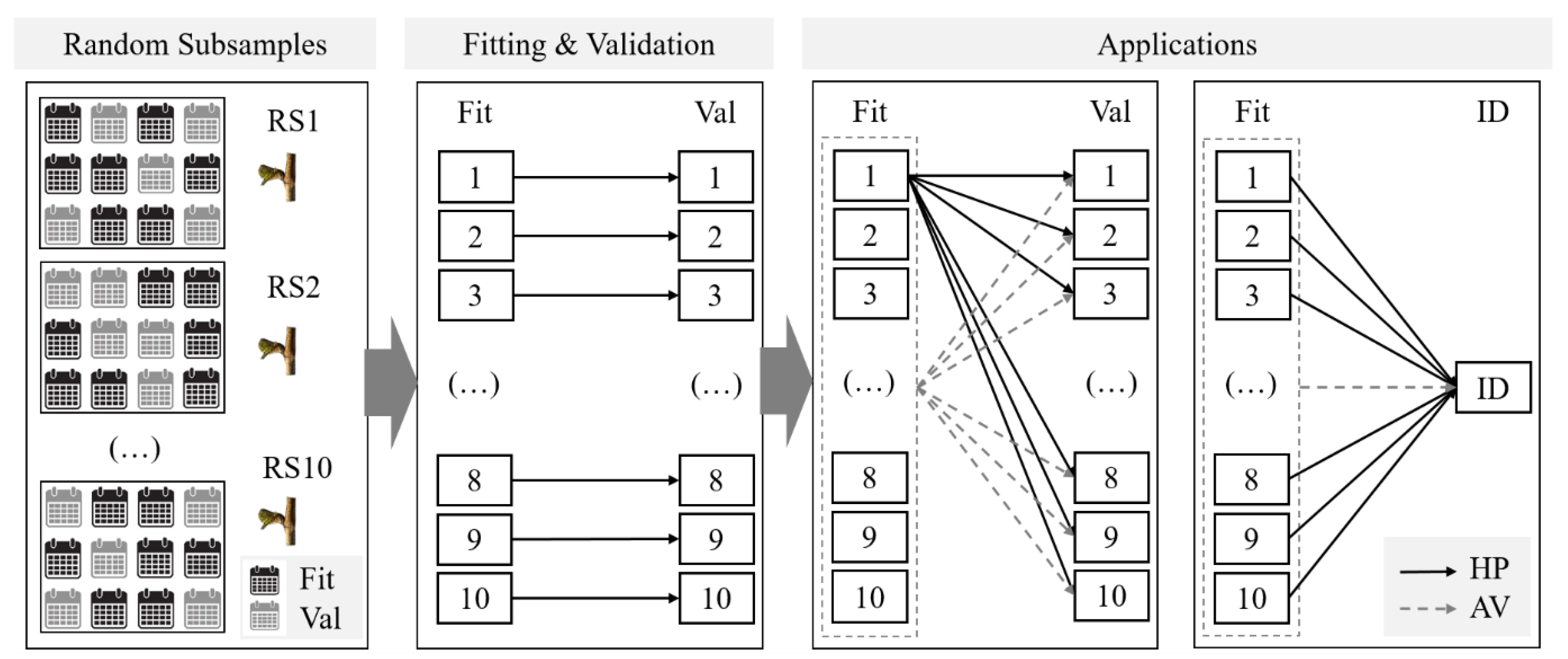
2.3. Model Fitting and Validation

2.3.1. Outliers Removal

The model fitting, validation and application were performed after removing outliers from the observed dataset. This procedure consists in the identification of possible anomalies by comparing the observed and simulated results obtained by a preliminary models’ fitting against the original datasets for each variety. The outliers were identified by using the Tukey method [43], based on the non-parametric measure of the statistical dispersion of a given distribution quantified using the interquartile range (IQR). For each model and starting date, the outliers represent the values in which the difference between the observed and simulated budbreak Days of Year (DOYs) are outside the whiskers of the distribution (below Q1 − 1.5 IQR or above Q3 + 1.5 IQR values). An outlier of a specific variety is removed from the dataset when it is observed in at least 4 combinations (models x starting date). The percentage of outliers removed from the fitting, validation and application datasets is: 4.17% (Cabernet Sauvignon), 5.36% (Chardonnay), 1.85% (Gewurztraminer and Riesling), 3.70% (Grenache), 1.52% (Pinot Gris), 10% (Touriga Franca and Nacional). These values were generally observed after extreme weather conditions (e.g., frosts of 1956, 1963 in France) or due to other influences (e.g., agronomic practices or errors in data collection) which cannot be reproduced during model simulation.

2.3.2. Parameters’ Range and Starting Date

The parameters’ range of variation in the 6 phenological models was defined according to the literature [29,30,44,45,46]. For the GDD model, the fitted parameter was T b which ranges from 0 to 10 °C. In this study, 0 °C was considered the limit temperature for bud growth while 10 °C was the maximum base temperature adopted for describing the eco-dormancy period as found in other studies [19,22,29,44]. For the WANG model, this function being generally used for wheat simulation [47], the parameter range of the cardinal temperatures was established considering the values obtained by other similar functions (Fbeta) implemented for simulating budbreak date in grapevine [30]. Thus, T min and T max were set at 0 and 45 °C respectively, while T o p t ranged in a ±30% of the value reported in Fila et al. [30]. For UNIFORC model, the d and e parameter values varied in a ±30% interval with respect to the average value reported for different grapevine varieties (Glera, Cabernet Sauvignon, Chardonnay and Merlot [46]). For both daily and hourly approaches of BRIN model, the Q 10 parameter range was defined in a ±30% interval of the value estimated for several grapevine varieties [29]. Moreover, the lower limit temperature ( T l ) was fitted in the range 0–10 °C, as reported for GDD model while the upper limit temperature ( T h ) for post dormancy was fixed at 25 °C as indicated in Garcia de Cortazar-Atauri et al. [29]. For the UNICHILL model, the parameters a , b , c , d and e were in a range of ±30% of the overall minimum and maximum value reported by Fila [46] for Glera, Cabernet Sauvignon, Chardonnay and Merlot varieties (field calibration). However, in the specific case of Cabernet Sauvignon and Chardonnay, the parameter range of a , b , c , d and e varied in ±30% interval with respect to the parameter values found for these varieties. Similarly, the range adopted for a, b , c , d and e parameters in UNIFIED model was identified by considering ±30% of the minimum and maximum values reported by Fila et al. [46] (field calibration). Based on the same study, the parameters w and z were fixed by considering the average values reported for field calibration of Sangiovese and Montepulciano.
Concerning the use of fixed starting dates t 0 during model simulation, we set the 1st of January [30] and 1st of March [27] of the current year for the F models and the 1st September [24] and 1st of August [29] of the previous year for the CF models.

2.3.3. Model Fitting, Validation and Application

The methodology used for model fitting, validation and application is displayed in Figure 2. After outliers removal (Section 2.3.1), the first step was to randomly split the observed data (budbreak DOY per year) into 10 random subsamples (RS) in which 60% of the observed data was used for model fitting whereas the remaining 40% was retained for validation. Once the 10 random subsamples were prepared, the model fitting was performed for any combination of varieties, models and starting dates using the Phenological Modeling Platform (PMP) software (version 5.5) [48] and setting the parameter ranges as described in Section 2.3.2. The best fitting for any combination was found by exploring the range of each parameter through the Metropolis-Hastings algorithm [49,50,51] of PMP. Each fitted model was validated on the remaining 40% of the data and then applied on the validation datasets of the other subsamples by using the R software environment (version 3.5.0) [52]. Thus, the parameter set of each model combination (model x variety x starting date), which provided the highest-performance (HP) during fitting and validation procedures, was selected. Moreover, the average parameter sets (AV) derived from all fitted subsamples was also tested on the entire distribution of validation datasets. Finally, the HP and AV parameter sets were applied to the independent datasets of other study sites to evaluate the behavior of different parameterizations under different environmental conditions.

2.4. Statistical Analysis

The statistical indices used for evaluating the phenological model performances during fitting, validation and application were: R-squared (R2, Equation (10), [53]); Akaike information criterion (AIC, Equation 11, [54]); Root Mean Squared Error (RMSE, Equation (12), [55]) and modeling efficiency coefficient (EF, Equation (13), [56]), each defined as follows:
R 2 = 1 i ( O i P i ) 2 i ( O i O ¯ ) 2 ,
A I C = 2 k 2 ln ( L ^ ) ,
R M S E = [ i = 1 n ( P i O i ) 2 n ] 0.5 ,
E F = 1 i = 1 n ( P i O i ) 2 i = 1 n ( O i O ¯ ) 2 ,
where Oi is the observed value, O ¯ is the average of the observed values, P i is the predicted value, n is the number of observations, k is the number of parameters in the model, and L ^ is the maximized value of the likelihood function of the predicted model.
Finally, the minimum, 10% quantile, median, mean, 90% quantile and maximum values of the statistics were extracted for describing the simulation results on all validation datasets.

3. Results

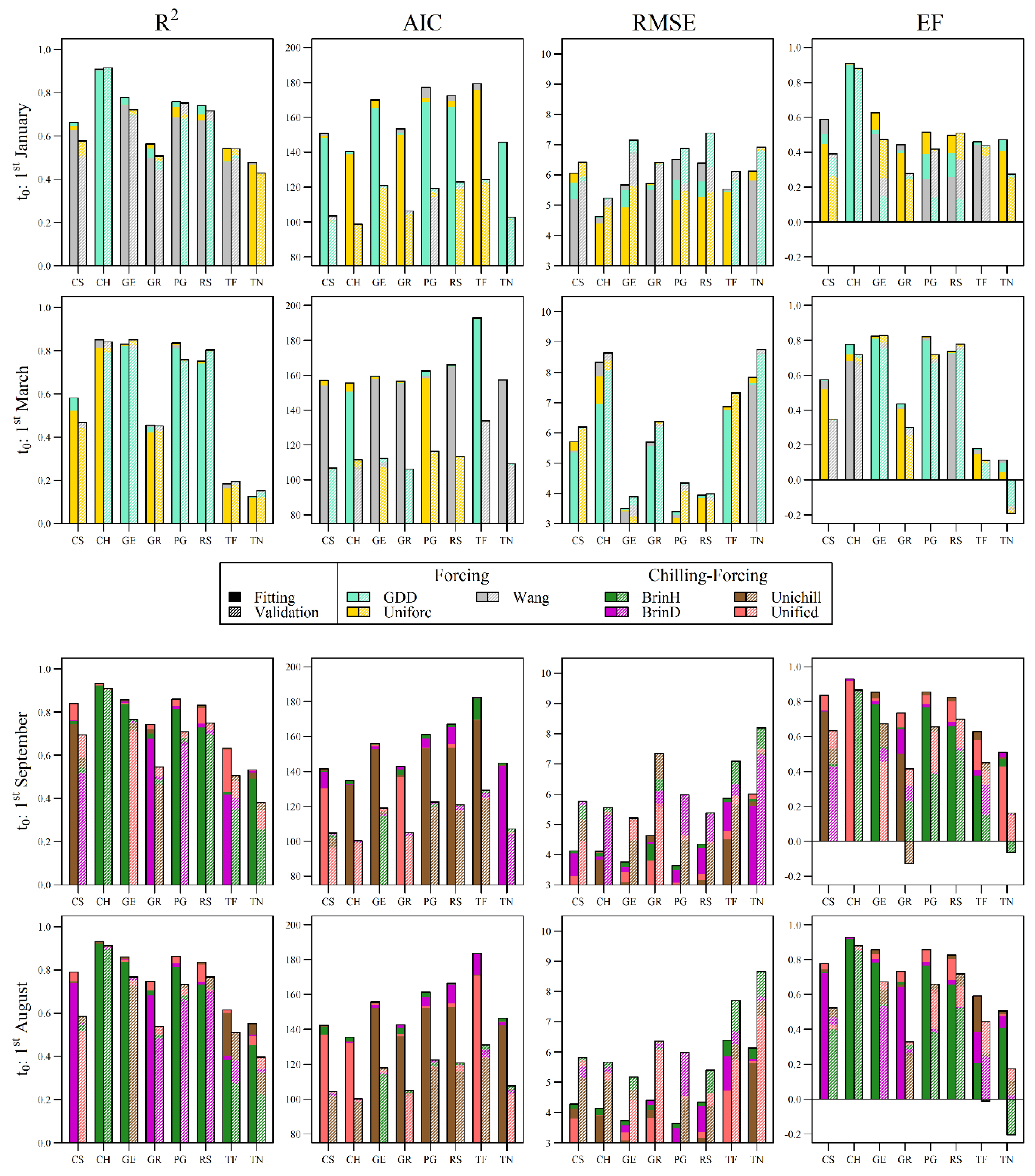
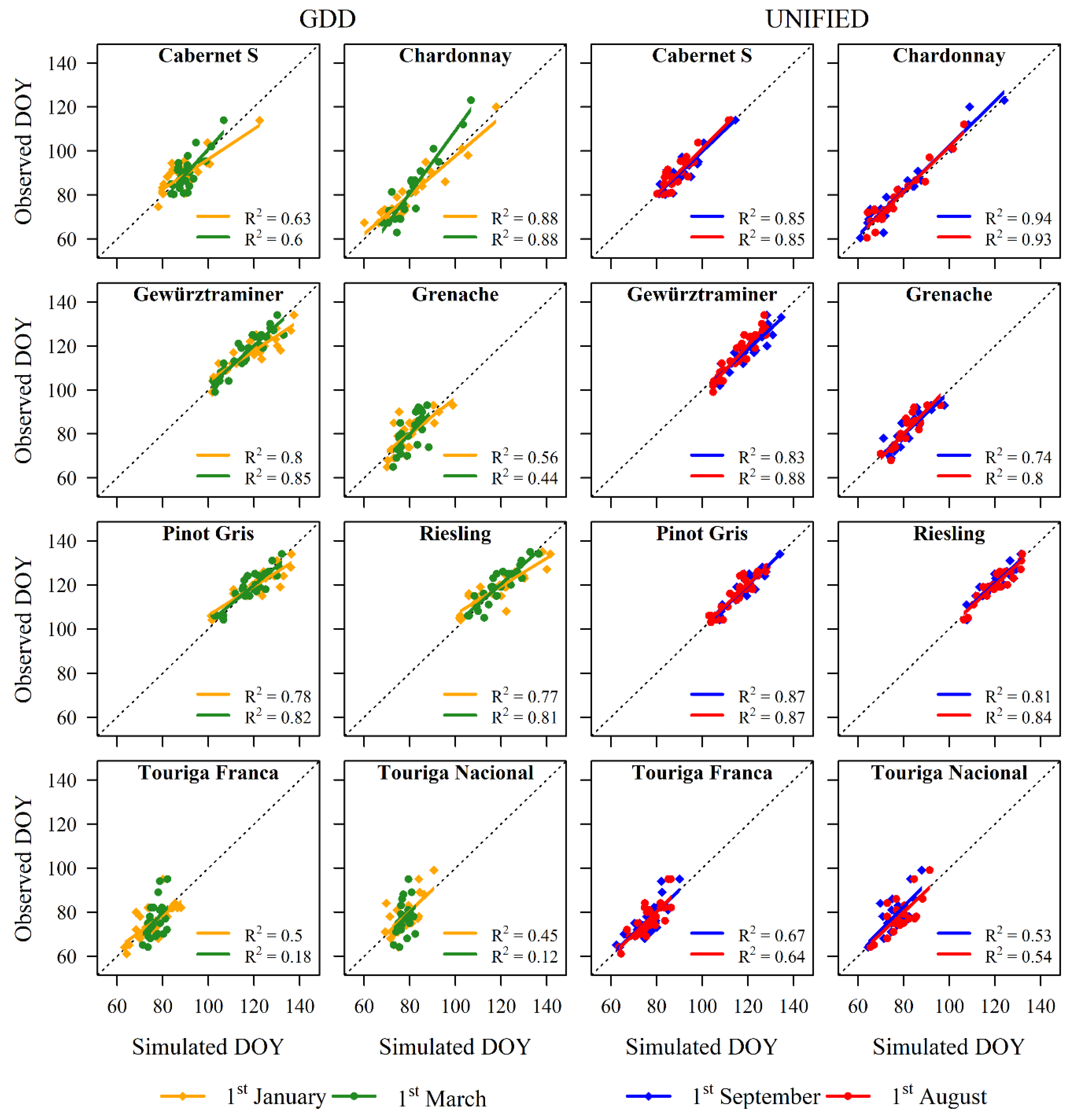
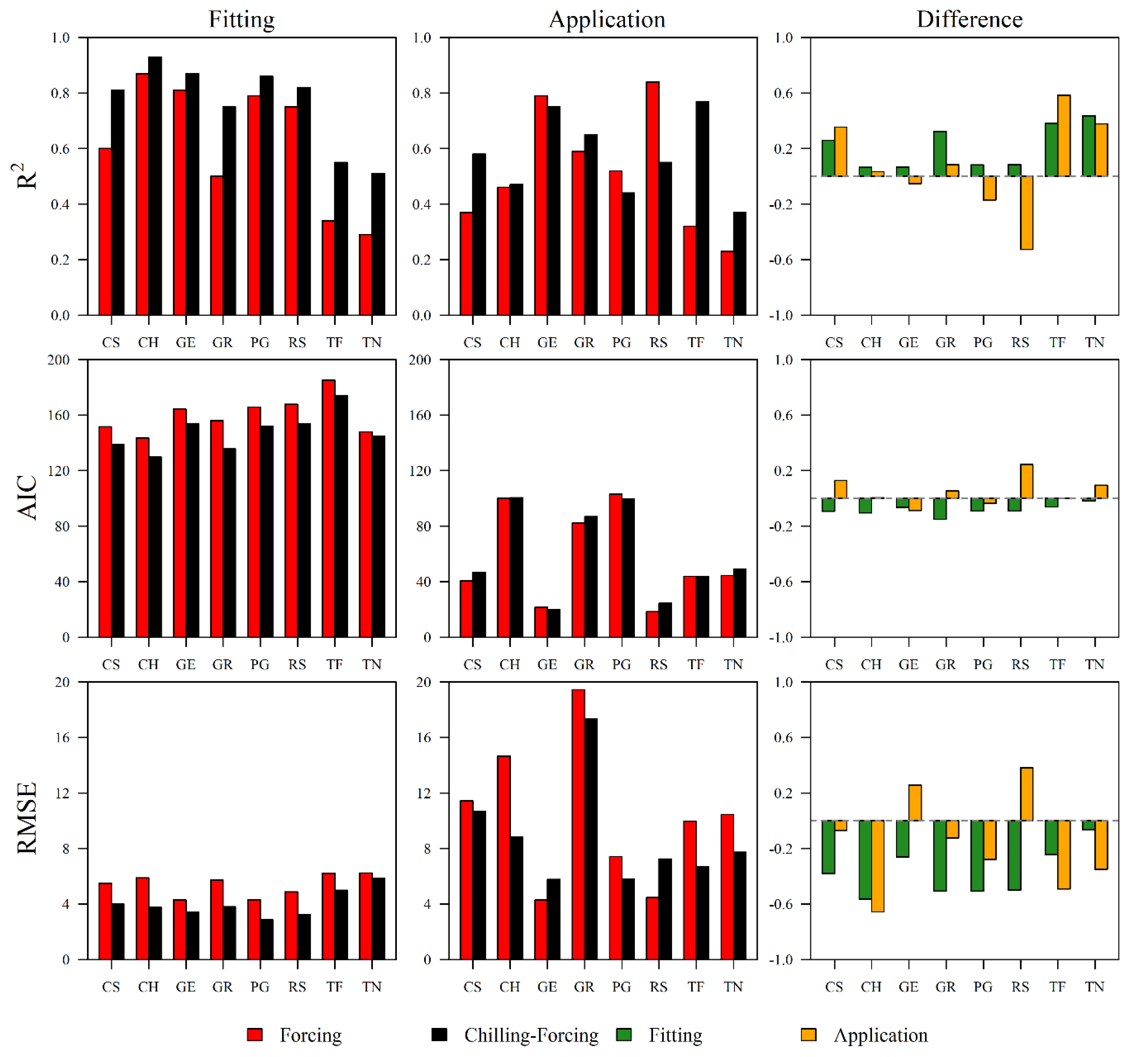
3.1. Overall Model Behavior in Fitting and Validation
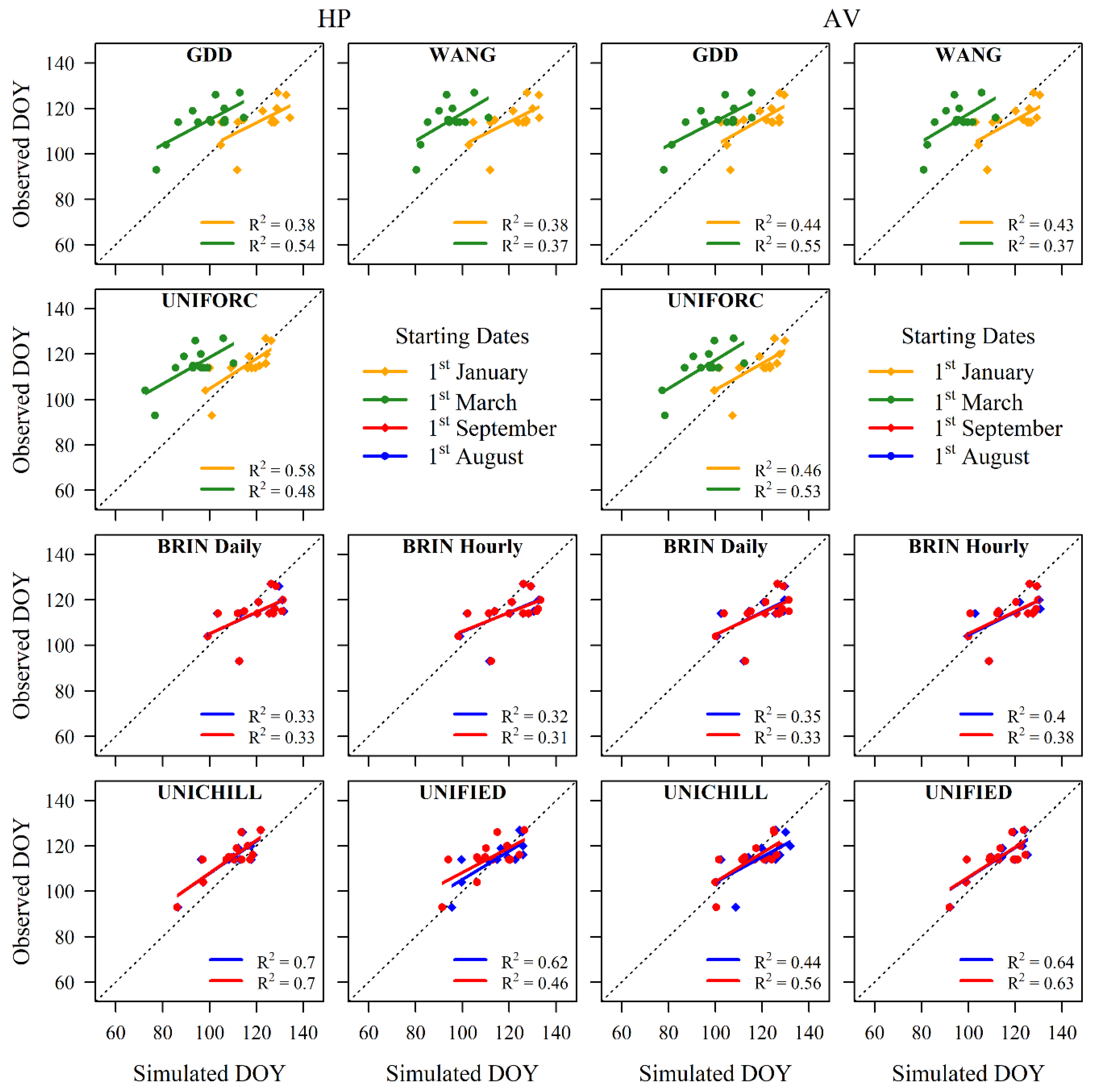
The results of the phenological model intercomparison were described comparing the performances of the different modeling approaches (e.g., F vs. CF) and starting dates (1st January/March vs. 1st September/August) during model fitting and validation. Initially, the model fitting and validation results evidenced higher average performances for CF (Fit, R2 = 0.74; AIC = 150.42; RMSE = 4.22, Val, R2 = 0.61; AIC = 111.64; RMSE = 5.79) compared to F models (Fit, R2 = 0.61; AIC = 160.62; RMSE = 5.51; Val, R2 = 0.59; AIC = 112.01; RMSE = 6.10). Among all models (Figure 3 and Table S1), the highest performances were achieved by UNIFIED model (Fit, R2 = 0.77; AIC = 147.60; RMSE = 3.96; Val, R2 = 0.64; AIC = 110.74; RMSE = 5.42), while the lowest were obtained by the WANG model (Fit, R2 = 0.61; AIC = 161.15; RMSE = 5.60) and GDD model (Val, R2 = 0.58; AIC = 112.59; RMSE = 6.25). Moreover, higher performances were found for those models in which the starting date was fixed at 1st September in CF models (Fit, R2 = 0.74; AIC = 150.24; RMSE = 4.21; Val, R2 = 0.61; AIC = 111.59; RMSE = 5.75) and at 1st January in F models (Fit, R2 = 0.66; AIC = 159.20; RMSE = 5.53; Val, R2 = 0.63; AIC = 111.10; RMSE = 6.15). Finally, concerning grapevine varieties, Chardonnay was best fitted by the models (Fit, R2 = 0.90; AIC = 138.66; RMSE = 4.90; Val, R2 = 0.89; AIC = 101.54; RMSE = 5.97), while the poorest results were obtained for Touriga Nacional (Fit, R2 = 0.42; AIC = 147.09; RMSE = 6.23; Val, R2 = 0.31; AIC = 105.40; RMSE = 7.74) and Touriga Franca in terms of AIC values (Fit = 180.19; Val = 127.35).

3.2. HP versus AV

In order to compare the results of different models’ parameterizations, we selected the highest performance parameter set (HP, Table 2) from the 10 fitting and validation subsamples for each combination of model, starting date and variety. We then selected the average parameter set (AV, Table 3) from the 10 fitting subsamples for each combination model, starting date and variety. On these bases, Figures S1–S7 show the performances (R2 and AIC) of the model fitting and validation (symbols) and the applications of the different parameterizations on all validation subsamples (boxplot) obtained by considering all grapevine varieties and starting dates. In detail, the selected parameter sets with highest performances (HP; filled symbols with different shapes according to the starting dates) were the result of the highest rank value of R2 and AIC and the minimum discrepancy between fitting (red) and validation (blue) models. By contrast, the AV parameter sets (boxplots in shadow area) were the application of the average parameterization obtained for all subsamples. Despite that similar performances for HP and AV parameter sets were evidenced in Figures S1–S7, higher discrepancy was found in the behavior of CF and F models. In Figures S1–S4 (CF models), no differences were observed when different starting dates were set during model fitting and application. On the other hand, high discrepancy was found in model performances when different starting dates were adopted in Figures S5–S7 (F models). This trend is also evidenced by the correlations between observed and simulated DOYs in Figure 4, Figures S8 and S9. The results of model fitting showed accurate performances for all selected HP, with more discrepancy between starting dates of F models (yellow and green correlations) compared to those used in CF models (blue and red correlations). The values of R2 also highlighted the higher performances obtained with some varieties compared to others (Chardonnay vs. Touriga Nacional).
A deeper analysis of the model validation showed that the normalized difference between HP and AV, (HP-AV/HP)*100, was higher in CF (R2 = 11.99%, AIC = 3.36%, RMSE = 22.20%) compared to F models (R2 = 5.73%, AIC = 1.51%, RMSE = 8.16%). Among CF models, UNICHILL model showed the lowest difference between HP and AV in terms of R2 and AIC (R2 = 6.20%, AIC = 2.70%), while it evidenced the highest difference in terms of RMSE (40.02%). Considering F models, WANG showed the highest difference (R2 = 7.07%, AIC = 2.25%, RMSE = 9.38%) and UNIFORC, the lowest (R2 = 4.21%, AIC = 0.84%, RMSE = 7.13%). Following the same trend, the starting dates 1st September and 1st August (R2 = 3.89%, AIC = 0.86%, RMSE = 15.62%) showed bigger differences compared to 1st January and 1st March (R2 = 2.96%, AIC = 0.72%, RMSE = 7.62%). In particular, 1st September showed a lower difference in terms of AIC and RMSE (AIC = 0.86%, RMSE = 13.53%) compared to 1st August in CF models while 1st January showed the highest difference in F models (R2 = 2.88%, AIC = 0.65%, RMSE = 7.23%). Finally, regarding grapevine varieties, the highest difference was found for Touriga Nacional (R2 = 23.96%, RMSE = 24.20%) while the lowest was shown by Chardonnay in terms of R2 (1.89%) and by Touriga Franca in terms of AIC and RMSE (1.10% and 9.55%, respectively).

3.3. Model Applications on Other Independent Datasets

The statistical performances of the phenological models, applied on the respective independent datasets, are reported in Figure 5 and Figures S10–S16 while the comparison between CF and F models during fitting and applications is shown in Figure 6 and Figure S17. In general, higher performances were found for CF compared to F models during fitting and applications (Figure 5), except for those varieties characterized by few observed data in the model application (Gewürztraminer, Riesling; Figure 6 and Figure S17).
In particular, the model application showed similar performances for both HP (R2 = 0.55, AIC = 57.97, RMSE = 9.41) and AV (R2 = 0.54, AIC = 58.37, RMSE = 9.26) parameter sets. However, this difference slightly increased when CF (R2 = 0.56, AIC = 59.05, RMSE = 8.75) and F models (R2 = 0.52, AIC = 57.01, RMSE = 10.01) were compared without distinguishing between HP and AV parameterizations. Therefore, CF models showed better results in terms of R2 (+8%) and RMSE (−15%) compared to F models while lower results of AIC value were obtained for CF compared to F models (+3.44%). A detailed analysis revealed that the CF models with highest performances (R2 and AIC) were UNICHILL (R2 = 0.64, AIC = 56.74) and UNIFIED (R2 = 0.58, AIC = 56.61) models, while, in F models, the better results were provided by UNIFORC (R2 = 0.54, AIC = 55.98). However, in terms of RMSE, highest performances were found for BRIN hourly (8.37, CF) and GDD (9.67, F). Concerning the starting dates, similar results were found when the 1st September (R2 = 0.58, AIC = 58.92, RMSE = 8.55) and 1st of August (R2 = 0.57, AIC = 59.17, RMSE = 8.95) were analyzed, with the 1st September showing better performance (R2 = +1.83%, AIC = −0.44% and RMSE = −4.68%). Instead, higher differences were found when the 1st January (R2 = 0.55, AIC = 60.47, RMSE = 7.74) and 1st of March (R2 = 0.49, AIC = 52.57, RMSE = 12.47) were compared, evidencing the most relevant performances for 1st January (R2 = +10.83% and RMSE = −61.23%, with the exception of AIC = +14.15%).
Moreover, the behavior of grapevine varieties in response to specific climate conditions was noticed during model application. The higher performances of CF compared to F, as well the relevant differences between starting dates when F models were used, may be explained by the influence of temperatures on the dormancy period. The end of the first phase of dormancy (endo-dormancy) in CF models was generally simulated between the end of December (e.g., Touriga Nacional: DOY 356 for t0 = −121 and −152, respectively) and end of February (e.g., Riesling: DOY 56 and 57 for t0 = −121 and −152, respectively). More specifically, the period of endo-dormancy fulfilment was similarly reached regardless of starting date (1st September/August), allowing the next forcing unit accumulation during the eco-dormancy period to be correctly satisfied (differences in days from 0 to 3 days). The analysis further highlighted that the endo-dormancy release occurs later at northern than at southern latitudes and this is consistent with results obtained using F approach. These demonstrate that a late starting date (1st of March) for forcing unit accumulation is more suitable for budbreak simulation of varieties collected in Northern Europe (e.g., Gewürztraminer, Riesling and Pinot Gris), whose endo-dormancy release is simulated by CF late in the season (54 DOY on average). Conversely, an early starting date (1 January) provided the best results in simulating budbreak for grapevine varieties collected in Southern Europe (e.g., Touriga Franca and Nacional, Cabernet Sauvignon, Grenache and Chardonnay), which are characterized by an early end of endo-dormancy as simulated by CF models (13 DOY on average).

4. Discussion

This study compares the performance of six phenological models in simulating the budbreak date of eight grapevine varieties across different European sites. We found that the model performances characterized by a Chilling-Forcing approach were generally higher compared to those obtained for Forcing approach when different starting dates were set (Figure 6 and Figure S17).
Although model intercomparison studies on the estimation of budbreak date in grapevine have already been conducted by other authors [15,29,30], this study focused on evaluation of the models’ reliability to reproduce budbreak in different environmental conditions, by considering the impact of temperature during the chilling and forcing accumulation period. In contrast to other works [27,30,57,58], this model intercomparison considers the use of a long-term series of observed phenology, which include grapevine varieties with different precocity levels collected at various latitudes in three European countries (France, Luxembourg and Portugal, Figure 1 and Table 1). The extensive observed dataset coupled to the methodology applied in this study allowed to evaluate the influence of study site-temperature variability on the grapevine development. Moreover, the cross-validation scheme adopted in this model intercomparison experiment provided an exhaustive analysis of the bias and variance of the CF and F models while the comparison between two different types of parameterization (HP or AV) pointed out the issue to select a specific parameter set for model applications (Results section, Figure 5). This in-depth investigation of model fitting, validation and application was particularly useful for evaluating the influence of temperature during the dormancy period. In this context, the different model responses during budbreak predictions are related to the physiological requirements needed for dormancy fulfilment of the grapevine varieties. Differently from the CF models, which describe the entire dormancy period (endo- and eco-dormancy), the F models only describe the eco-dormancy period through forcing units accumulation, under the assumption that the chilling requirement was already satisfied [24]. Although the debate on which model type provides the highest reliability is still open [29,30], our analysis shows that CF models, considering the influences of winter and spring temperatures on the accumulation of chilling and forcing units, may avoid the under- or over-estimation at the beginning of eco-dormancy, which occur when F models are set on fixed dates. In this study, we estimated a longer endo-dormancy for the vines from the Northern European sites (e.g., Gewürztraminer), which occurs later than the endo-dormancy of vines from the Southern European sites (e.g., Touriga Nacional), irrespective of the precocity level of the different varieties. In other terms, grapevine varieties such as Gewürztraminer (early budbreak) and Riesling (late budbreak) collected in Northern Europe showed a late endo-dormancy release (higher chilling requirement) with respect to Chardonnay (early budbreak) and Cabernet Sauvignon (late budbreak) mainly collected in Southern Europe (lower chilling requirement). Although this trend was examined in this study only from a modeling point of view without any physiological evidence on the dormancy period, our results suggested that plants cultivated at different latitudes might show distinct dormancy period lengths. The higher accuracy of CF compared to F models is likely linked to the ability of these models to estimate the endo-dormancy release and to better account for the effect of temperature in this phase, avoiding the use of a fixed a priori value for the beginning of the eco-dormancy period as in F models [27,29]. Indeed, the goodness of F models is shown to significantly increase when the starting date is optimized against observed experimental data [30,45], demonstrating that the beginning of eco-dormancy period is dependent to the origin of the observed dataset and, thus, on the fulfilment of specific physiological requirements that change in relation to the climate conditions of the different environments. In fact, although no relevant differences were found for budbreak date estimation of grapevine varieties using CF models set on 1st of September/August starting dates, the discrepancy of the F model simulations was evident when 1st of January/March dates were used. Higher accuracy of F models to predict the budbreak date of grapevine varieties collected in Northern European countries was observed using the 1st of March starting date as also confirmed by [27], while the 1st January seems to be a more suitable starting date for representing budbreak date of the grapevine varieties from Southern Europe (Figures S5–S7). In this case, a compromise between both starting dates may be represented by the beginning of February [59]. However, the adoption of different starting dates in F models highlights the role of temperature on bud growth and the need to satisfy specific dormancy requirements for varieties cultivated at different latitudes before budbreak occurrence. These results were supported by the work of Reis-Pereira et al. [60] on the grapevine flowering stage. The authors pointed out that the selection of a priori value for the starting of thermal unit accumulation in F models may lead to an under- or over-estimation of the flowering phase, demonstrating the importance of a correct evaluation of the previous phenological stage in respect to the subsequent one. These findings were also observed in relation to the flowering stage of other species such as olive tree e.g., [61]). In this context, we infer that the dormancy period of grapevine may play a relevant role for predicting budbreak date especially under future scenarios. Indeed, more accurate estimations of budbreak date using CF models are provided when the endo-dormancy release is calibrated against observed data of perennial crops. This behavior is particularly evident under warmer temperatures (after 2050) where CF without endo-dormancy calibration and F models showed poor performances of phenology prediction [62]. The accurate identification of the endo-dormancy release avoids selecting a fixed a priori date, especially when this may have strong consequences on the estimation of budbreak date (as in F models).
The impact of warmer temperatures after the endo-dormancy release showed higher effect on the budbreak phase compared to the influence of temperatures during chilling accumulation, as reported by Martinez-Lüscher et al. [63] in a two-year ad hoc experiment with different grapevine varieties and temperature regimes. However, the starting date for thermal unit accumulation depends on the physiological features of the grapevine variety and their interaction with the environment. Indeed, we found that the effect of temperature during the last part of winter and beginning of spring was also evident when models were tested on external sites (independent datasets, Figure 5). Although most of the models showed satisfactory results during application (R2 and AIC), the average error (RMSE) between observed and simulated data was relatively high (from 4 to 19 days). This situation was exacerbated in F models where the reliability in simulating budbreak is dependent to the use of a specific starting date (1st of January/1st of March) and thus the original observed dataset. The discrepancy between the two starting dates raises the question of which initial date to choose for forcing unit accumulation when simulations are conducted on a European scale [31,64].
The implications of this study are particularly relevant for growers especially when considering the impact of climate change. Our study, in line with a large part of literature, confirmed that chill units accumulations, the amount of which varies according to variety and location, is required for exiting from endo-dormancy phase. In a warmer climate, as expected in the future, this amount may not fully satisfy, leading to developmental issues during the growing season as outlined in the introduction of this paper. Some authors already highlighted that, on a global scale, wine areas may shift to match their specific climate niches in case of no adaptation [11,65], while new varietal selections and breeding programmes are needed for improving the adaptability of the grapevine varieties and maintaining the high quality production [12,59,66]. In this context, our parameterizations may be used as metric, in combination with climate simulations under future scenarios, to highlight which regions and varieties are expected to be most exposed to the risk of budbreak failure. Accordingly, the use of alternative varieties, better adapted to the expected future climate, may be proposed or the direction of specific breeding programmes can be indicated to develop varieties with a lower chill units requirement as requested in a warmer climate. Moreover, we should also take into account that, besides thermal requirements, dormancy phase may be influenced by the photoperiod [67]. Since each grapevine variety requires critical thresholds of day length for the onset of dormancy [68,69], this regulating factor should be considered when CF models are adopted for simulations at different latitudes. As such, comprehensive datasets of phenological observations and ad hoc experiments for evaluating the influence of more factors on dormancy [30,46,69] may be useful to take into account for improving model reliability under future climate scenarios and different environments [31,64,70].

5. Conclusions

This model intercomparison evidenced the different performance of the phenological models in reproducing the budbreak date of eight grapevine varieties collected in different European regions. The reliability of two main phenological modeling approaches (CF and F) was evaluated considering different starting dates (1st January/March or 1st September/August) and the selection methodologies of the parameter set (HP and AV) for model application. The results showed, in general, higher performances of CF compared to F models where fixed starting dates were adopted, even if neither modeling approach highlighted a clear supremacy over the other. For this reason, CF and F models’ behavior should be further investigated through ad hoc experiments for evaluating the role of dormancy on budbreak occurrence. Indeed, the findings of our model simulations evidenced distinct thermal requirements for grapevine varieties cultivated at different latitudes (i.e., Northern Europe vs. Southern Europe). The use of different starting dates highlighted that, unlike CF models, the accurate estimation of budbreak in F models is affected by the selection of a starting date for beginning of the eco-dormancy period. This implies that, if this phase is not accurately defined, F models may lead to over- or under-estimations of the budbreak date under different environmental conditions. In this context, comprehensive phenological datasets (e.g., grapevine phenological data collected at different latitudes) are needed to thoroughly investigate the effect of temperature variability on dormancy period and budbreak estimation. Finally, it is proposed the development and implementation of improved phenological models, which consider the effect of other climate (e.g., radiation) and soil (e.g., soil temperature) variables as well as some regulating factors of the endo-dormancy phase (e.g., day length).

Supplementary Materials

The following are available online at https://0-www-mdpi-com.brum.beds.ac.uk/2076-3417/10/11/3800/s1. Figure S1: R2 and AIC values of the BRIN Daily model obtained for all fitted and average models, grapevine varieties and starting dates. The symbols (points and triangles) show the model results at two starting dates (in this example t0 = −121 and −152 DOY), while the two colours represent fitting (red) and validation (blue) procedure, respectively. The filled symbols constitute the R2 and AIC values of the models obtained by the selected HP parameter sets, while the dashed (fitting) and dotted (validation) lines depict the average R2 and AIC values for both starting dates (in this example orange line = −121 DOY and green line = −152 DOY). The boxplots represent the R2 and AIC values distribution for HP (orange and light blue: HP model application on all validation subsamples for t0 = −121 and t0 = −152 DOY, respectively) and AV (boxplot in the shaded area, orange and light blue: AV application on all validation subsamples for t0 = −121 and t0 = −152 DOY, respectively). The outliers represent all values out of the 1.5*InterQuartile Range (IQR) of the boxplot. Figure S2: R2 and AIC values of the BRIN Hourly model obtained for all fitted and average models, grapevine varieties and starting dates. The symbols (points and triangles) show the model results at two starting dates (in this example t0 = −121 and −152 DOY), while the two colours represent fitting (red) and validation (blue) procedure, respectively. The filled symbols constitute the R2 and AIC values of the models obtained by the selected HP parameter sets, while the dashed (fitting) and dotted (validation) lines depict the average R2 and AIC values for both starting dates (in this example orange line = −121 DOY and green line = −152 DOY). The boxplots represent the R2 and AIC values distribution for HP (orange and light blue: HP model application on all validation subsamples for t0 = −121 and t0 = −152 DOY, respectively) and AV (boxplot in the shaded area, orange and light blue: AV application on all validation subsamples for t0 = −121 and t0 = −152 DOY, respectively). The outliers represent all values out of the 1.5*InterQuartile Range (IQR) of the boxplot. Figure S3: R2 and AIC values of the UNICHILL model obtained for all fitted and average models, grapevine varieties and starting dates. The symbols (points and triangles) show the model results at two starting dates (in this example t0 = −121 and −152 DOY), while the two colours represent fitting (red) and validation (blue) procedure, respectively. The filled symbols constitute the R2 and AIC values of the models obtained by the selected HP parameter sets, while the dashed (fitting) and dotted (validation) lines depict the average R2 and AIC values for both starting dates (in this example orange line = −121 DOY and green line = −152 DOY). The boxplots represent the R2 and AIC values distribution for HP (orange and light blue: HP model application on all validation subsamples for t0 = −121 and t0 = −152 DOY, respectively) and AV (boxplot in the shaded area, orange and light blue: AV application on all validation subsamples for t0 = −121 and t0 = −152 DOY, respectively). The outliers represent all values out of the 1.5*InterQuartile Range (IQR) of the boxplot. Figure S4: R2 and AIC values of the UNIFIED model obtained for all fitted and average models, grapevine varieties and starting dates. The symbols (points and triangles) show the model results at two starting dates (in this example t0 = −121 and −152 DOY), while the two colours represent fitting (red) and validation (blue) procedure, respectively. The filled symbols constitute the R2 and AIC values of the models obtained by the selected HP parameter sets, while the dashed (fitting) and dotted (validation) lines depict the average R2 and AIC values for both starting dates (in this example orange line = −121 DOY and green line = −152 DOY). The boxplots represent the R2 and AIC values distribution for HP (orange and light blue: HP model application on all validation subsamples for t0 = −121 and t0 = −152 DOY, respectively) and AV (boxplot in the shaded area, orange and light blue: AV application on all validation subsamples for t0 = −121 and t0 = −152 DOY, respectively). The outliers represent all values out of the 1.5*InterQuartile Range (IQR) of the boxplot. Figure S5: R2 and AIC values of the UNIFORC model obtained for all fitted and average models, grapevine varieties and starting dates. The symbols (points and triangles) show the model results at two starting dates (in this example t0 = 1 and 60 DOY), while the two colours represent fitting (red) and validation (blue) procedure, respectively. The filled symbols constitute the R2 and AIC values of the models obtained by the selected HP parameter sets, while the dashed (fitting) and dotted (validation) lines depict the average R2 and AIC values for both starting dates (in this example orange line = 1 DOY and green line = 60 DOY). The boxplots represent the R2 and AIC values distribution for HP (orange and light blue: HP model application on all validation subsamples for t0 = 1 and t0 = 60 DOY, respectively) and AV (boxplot in the shaded area, orange and light blue: AV application on all validation subsamples for t0 = 1 and t0 = 60 DOY, respectively). The outliers represent all values out of the 1.5*InterQuartile Range (IQR) of the boxplot. Figure S6: R2 and AIC values of the GDD model obtained for all fitted and average models, grapevine varieties and starting dates. The symbols (points and triangles) show the model results at two starting dates (in this example t0 = 1 and 60 DOY), while the two colours represent fitting (red) and validation (blue) procedure, respectively. The filled symbols constitute the R2 and AIC values of the models obtained by the selected HP parameter sets, while the dashed (fitting) and dotted (validation) lines depict the average R2 and AIC values for both starting dates (in this example orange line = 1 DOY and green line = 60 DOY). The boxplots represent the R2 and AIC values distribution for HP (orange and light blue: HP model application on all validation subsamples for t0 = 1 and t0 = 60 DOY, respectively) and AV (boxplot in the shaded area, orange and light blue: AV application on all validation subsamples for t0 = 1 and t0 = 60 DOY, respectively). The outliers represent all values out of the 1.5*InterQuartile Range (IQR) of the boxplot. Figure S7: R2 and AIC values of the WANG model obtained for all fitted and average models, grapevine varieties and starting dates. The symbols (points and triangles) show the model results at two starting dates (in this example t0 = 1 and 60 DOY), while the two colours represent fitting (red) and validation (blue) procedure, respectively. The filled symbols constitute the R2 and AIC values of the models obtained by the selected HP parameter sets, while the dashed (fitting) and dotted (validation) lines depict the average R2 and AIC values for both starting dates (in this example orange line = 1 DOY and green line = 60 DOY). The boxplots represent the R2 and AIC values distribution for HP (orange and light blue: HP model application on all validation subsamples for t0 = 1 and t0 = 60 DOY, respectively) and AV (boxplot in the shaded area, orange and light blue: AV application on all validation subsamples for t0 = 1 and t0 = 60 DOY, respectively). The outliers represent all values out of the 1.5*InterQuartile Range (IQR) of the boxplot. Figure S8: Correlations between observed and simulated budbreak Days of Year (DOY) of the UNIFORC and UNICHILL models. The results were obtained for all grapevine varieties and starting dates using the HP parameter set. Figure S9: Correlations between observed and simulated budbreak Days of Year (DOY) of the WANG and BRIN Daily models. The results were obtained for all grapevine varieties and starting dates using the HP parameter set. Figure S10: Highest-Performance (HP) and average (AV) parameters’ set applied on the independent datasets by considering all phenological models and starting dates. The example of Cabernet sauvignon variety. Figure S11: Highest-Performance (HP) and average (AV) parameters’ set applied on the independent datasets by considering all phenological models and starting dates. The example of Gewürztraminer variety. Figure S12: Highest-Performance (HP) and average (AV) parameters’ set applied on the independent datasets by considering all phenological models and starting dates. The example of Grenache variety. Figure S13: Highest-Performance (HP) and average (AV) parameters’ set applied on the independent datasets by considering all phenological models and starting dates. The example of Pinot Gris variety. Figure S14: Highest-Performance (HP) and average (AV) parameters’ set applied on the independent datasets by considering all phenological models and starting dates. The example of Riesling variety. Figure S15: Highest-Performance (HP) and average (AV) parameters’ set applied on the independent datasets by considering all phenological models and starting dates. The example of Touriga Franca variety. Figure S16: Highest-Performance (HP) and average (AV) parameters’ set applied on the independent datasets by considering all phenological models and starting dates. The example of Touriga Nacional variety. Figure S17: Statistical results (R2, AIC and RMSE) of the comparison between CF (black bars) and F (red bars) models in model fitting and application for all grapevine varieties using AV parameters’ set. The differences between CF and F models in model fitting and applications were displayed using green and yellow bars, respectively. CS = Cabernet Sauvignon, CH = Chardonnay, GE = Gewürztraminer, GR = Grenache, PG = Pinot Gris, RS = Riesling, TF = Touriga Franca, TN = Touriga Nacional. Table S1: Statistical indices (RMSE, EF, R2, AIC) obtained for all models, varieties and starting dates after model fitting and validation on all subsamples.

Author Contributions

Conceptualization, L.L., S.C.-A., J.A.S. and M.M.; methodology, L.L., S.C.-A., C.M., M.M., H.F., C.v.L., P.M.; data provision, D.M., J.J., A.D.-I., C.v.L., J.A.S., J.E.-D. and J.S.; writing—original draft preparation, L.L. and S.C.-A.; writing—review and editing, L.L., S.C.-A., J.A.S., C.M., H.F., D.M., P.M., J.J., T.K., A.D.-I., C.v.L., A.C.M., C.D., M.B. and M.M.; supervision, M.M.; funding acquisition, M.B. All authors have read and agreed to the published version of the manuscript.

Funding

This research was funded by the European Union’s Horizon 2020 Research and Innovation Programme, under the Clim4Vitis project: “Climate change impact mitigation for European viticulture: knowledge transfer for an integrated approach”, grant agreement no. 810176. It was also supported by FCT-Portuguese Foundation for Science and Technology, under the project UIDB/04033/2020 and the French National Research Agency (ANR) in the frame of the Investments for the Future Program, within the cluster of excellence COTE (ANR-10-LABX-45).

Acknowledgments

We wish to acknowledge the Clim4Vitis project “Climate change impact mitigation for European viticulture: knowledge transfer for an integrated approach”, funded by European Union’s Horizon 2020 Research and Innovation Program, under grant agreement no. 810176 that supported this study. H.F. thanks the FCT for contract CEECIND/00447/2017 and project COA/CAC/0030/2019.

Conflicts of Interest

The authors declare no conflict of interest.

References

  1. Mullins, M.G.; Bouquet, A.; Williams, L.E. Biology of the Grapevine; Cambridge University Press: Cambridge, UK, 1992. [Google Scholar]
  2. Van Leeuwen, C.; Seguin, G. The concept of terroir in viticulture. J. Wine Res. 2006, 17, 1–10. [Google Scholar] [CrossRef]
  3. Jones, G.V. Winegrape phenology. In Phenology: An Integrative Environmental Science; Schwartz, M.D., Ed.; Springer: Dordrecht, The Nederlands, 2013; pp. 563–584. [Google Scholar]
  4. Jones, G.V.; Davis, R.E. Climate influences on grapevine phenology, grape composition, and wine production and quality for Bordeaux, France. Am. J. Enol. Vitic. 2000, 51, 249–261. [Google Scholar]
  5. Menzel, A. A 500 year pheno-climatological view on the 2003 heatwave in Europe assessed by grape harvest dates. Meteorol. Zeitschrift 2005, 14, 75–77. [Google Scholar]
  6. Tomasi, D.; Jones, G.V.; Giust, M.; Lovat, L.; Gaiotti, F. Grapevine Phenology and Climate Change: Relationships and Trends in the Veneto Region of Italy for 1964-2009. Am. J. Enol. Vitic. 2011, 62, 329–339. [Google Scholar]
  7. Van Leeuwen, C.; Destrac-Irvine, A.; Dubernet, M.; Duchêne, E.; Gowdy, M.; Marguerit, E.; Pieri, P.; Parker, A.; de Rességuier, L.; Ollat, N. An Update on the Impact of Climate Change in Viticulture and Potential Adaptations. Agronomy 2019, 9, 514. [Google Scholar] [CrossRef] [Green Version]
  8. Ramos, M.C.; Jones, G.V.; Martínez-Casasnovas, J.A. Structure and trends in climate parameters affecting winegrape production in northeast Spain. Clim. Res. 2008, 38, 1–15. [Google Scholar] [CrossRef] [Green Version]
  9. Moriondo, M.; Bindi, M.; Fagarazzi, C.; Ferrise, R.; Trombi, G. Framework for high-resolution climate change impact assessment on grapevines at a regional scale. Reg. Environ. Chang. 2011, 11, 553–567. [Google Scholar]
  10. Gaál, M.; Moriondo, M.; Bindi, M. Modelling the impact of climate change on the Hungarian wine regions using Random Forest. Appl. Ecol. Environ. Res. 2012, 10, 121–140. [Google Scholar]
  11. Moriondo, M.; Jones, G.V.; Bois, B.; Dibari, C.; Ferrise, R.; Trombi, G.; Bindi, M. Projected shifts of wine regions in response to climate change. Clim. Change 2013, 119, 825–839. [Google Scholar] [CrossRef]
  12. Wolkovich, E.M.; García de Cortázar-Atauri, I.; Morales-Castilla, I.; Nicholas, K.A.; Lacombe, T. From Pinot to Xinomavro in the world’s future wine-growing regions. Nat. Clim. Chang. 2018, 8, 29–37. [Google Scholar] [CrossRef]
  13. Fraga, H.; Pinto, J.G.; Santos, J.A. Climate change projections for chilling and heat forcing conditions in European vineyards and olive orchards: A multi-model assessment. Clim. Chang. 2019, 152, 179–193. [Google Scholar] [CrossRef]
  14. Malheiro, A.C.; Campos, R.; Fraga, H.; Eiras-Dias, J.; Silvestre, J.; Santos, J.A. Winegrape phenology and temperature relationships in the Lisbon wine region, Portugal. J. Int. Sci. Vigne Vin 2013, 47, 287–299. [Google Scholar]
  15. Costa, R.; Fraga, H.; Fonseca, A.; De Cortázar-Atauri, I.G.; Val, M.C.; Carlos, C.; Reis, S.; Santos, J.A. Grapevine phenology of cv. Touriga Franca and Touriga Nacional in the Douro wine region: Modelling and climate change projections. Agronomy 2019, 9, 1–20. [Google Scholar]
  16. Molitor, D.; Junk, J. Climate change is implicating a two-fold impact on air temperature increase in the ripening period under the conditions of the Luxembourgish grapegrowing region. OENO One 2019, 53, 409–422. [Google Scholar] [CrossRef]
  17. Shulman, Y.; Nir, G.; Fanberstein, L.; Lavee, S. The effect of cyanamide on the release from dormancy of grapevine buds. Sci. Hortic. (Amsterdam) 1983, 19, 97–104. [Google Scholar]
  18. Wicks, A.S.; Johnson, J.O.; Bracho, E.; Jensen, F.L.; Neja, R.A.; Lider, L.A.; Weaver, R.J. Induction of early and more uniform budbreak in Vitis vinifera L. cvs. Perlette, Thompson Seedless, and Flame Seedless. In Proceedings of the Bud Dormancy in Grapevine: Potential and Practical Uses of Hydrogen Cyanamide on Grapevine, Fresno, CA, USA, 20 August 1984; Weaver, R.J., Ed.; University of California: Fresno, CA, USA, 1984; pp. 48–58. [Google Scholar]
  19. Dokoozlian, N.K. Chilling temperature and duration interact on the budbreak of “Perlette” grapevine cuttings. HortScience 1999, 34, 1054–1056. [Google Scholar] [CrossRef] [Green Version]
  20. Sarvas, R. Investigations on the annual cycle of development of forest trees. Autumn dormancy and winter dormancy. Commun. Inst. For. Fenn. 1974, 84, 1–101. [Google Scholar]
  21. Pouget, R. Considérations Générales sur le rythme végétatif et la dormance des bourgeons de la Vigne. Vitis 1972, 217, 198–217. [Google Scholar]
  22. Pouget, R. Nouvelle conception du seuil de croissance chez la vigne. Vitis 1968, 7, 201–205. [Google Scholar]
  23. Richardson, E.A.; Seeley, S.D.; Walker, D.R.; Walker, D.I. A model for estimating the completion of rest for “Redhaven” and “Elberta” peach trees. Hortic. Sci. 1974, 9, 331–332. [Google Scholar]
  24. Chuine, I. A unified model for budburst of trees. J. Theor. Biol. 2000, 207, 337–347. [Google Scholar] [CrossRef] [PubMed]
  25. Cesaraccio, C.; Spano, D.; Snyder, R.L.; Duce, P. Chilling and forcing model to predict bud-burst of crop and forest species. Agric. For. Meteorol. 2004, 126, 1–13. [Google Scholar] [CrossRef]
  26. Garcia de Cortazar-Atauri, I.; Brisson, N.; Seguin, B.; Gaudillere, J.; Baculat, E. Simulation of budbreak date for vine. The bring model. Some application in climate change study. In Proceedings of the XIV International GESCO Viticulture Congress, Geisenheim, Germany, 23–27 August 2005; pp. 485–490. [Google Scholar]
  27. Nendel, C. Grapevine bud break prediction for cool winter climates. Int. J. Biometeorol. 2010, 54, 231–241. [Google Scholar] [CrossRef]
  28. Caffarra, A.; Eccel, E. Projecting the impacts of climate change on the phenology of grapevine in a mountain area. Aust. J. Grape Wine Res. 2011, 17, 52–61. [Google Scholar] [CrossRef]
  29. García de Cortázar-Atauri, I.; Brisson, N.; Gaudillere, J.P. Performance of several models for predicting budburst date of grapevine (Vitis vinifera L.). Int. J. Biometeorol. 2009, 53, 317–326. [Google Scholar] [CrossRef]
  30. Fila, G.; Gardiman, M.; Belvini, P.; Meggio, F.; Pitacco, A. A comparison of different modelling solutions for studying grapevine phenology under present and future climate scenarios. Agric. For. Meteorol. 2014, 195–196, 192–205. [Google Scholar] [CrossRef]
  31. Leolini, L.; Moriondo, M.; Fila, G.; Costafreda-Aumedes, S.; Ferrise, R.; Bindi, M. Late spring frost impacts on future grapevine distribution in Europe. Field Crops Res. 2018, 222, 197–208. [Google Scholar] [CrossRef]
  32. Moriondo, M.; Ferrise, R.; Trombi, G.; Brilli, L.; Dibari, C.; Bindi, M. Environmental Modelling & Software Modelling olive trees and grapevines in a changing climate *. Environ. Model. Softw. 2015, 72, 387–401. [Google Scholar]
  33. Molitor, D.; Junk, J.; Evers, D.; Hoffmann, L.; Beyer, M. A high-resolution cumulative degree day-based model to simulate phenological development of grapevine. Am. J. Enol. Vitic. 2014, 65, 72–80. [Google Scholar] [CrossRef]
  34. Menne, M.J.; Durre, I.; Vose, R.S.; Gleason, B.E.; Houston, T.G. An overview of the global historical climatology network-daily database. J. Atmos. Ocean. Technol. 2012, 29, 897–910. [Google Scholar] [CrossRef]
  35. Destrac-Irvine, A.; van Leeuwen, C. VitAdapt: An experimental program to study the behavior of a wide range of Vitis vinifera varieties in a context of climate change in the Bordeaux vineyards. In Proceedings of the Sustainable Grape and Wine Production in the Context of Climate Change. ClimWine 2016 International Symposium, Bordeaux, France, 10–13 April 2016. [Google Scholar]
  36. Garcia de Cortazar-Atauri, I.; Audergon, J.M.; Delzon, S.; Anger, C.; Duchêne, E.; Bonhomme, M.; Legave, J.M.; Chuine, I.; Raynal, H.; Davi, H.; et al. PERPHECLIM ACCAF Project-perennial fruit crops and forest phenology evolution facing climatic changes. In Proceedings of the XVI International Sumposium on Apricot Breeding and Culture and XV Chinese National Symposium on Plum and Apricot, Shenyang, China, 29 June–3 July 2015. [Google Scholar]
  37. Jones, G.V. Climate and Terroir: Impacts of Climate Variability and Change on Wine. In Fine Wine and Terroir-the Geoscience Perspective; Meinert, L.D., Ed.; Geological Association of Canada: St. John’s, NL, Canada, 2006; p. 247. [Google Scholar]
  38. Eichhorn, V.K.W.; Lorenz, D.H. Phänologische Entwicklungsstadien der Rebe [Phenological development stages of the grapevine]. Nachr. Dtsch. Pflanzenschutzd. 1977, 29, 119–120. [Google Scholar]
  39. Amerine, M.A.; Winkler, A.J. Composition and Quality of Musts and Wines of California Grapes. Hilgardia 1944, 15, 493–675. [Google Scholar] [CrossRef] [Green Version]
  40. Wang, E.; Engel, T. Simulation of phenological development of wheat crops. Agric. Syst. 1998, 58, 1–24. [Google Scholar] [CrossRef]
  41. Bidabe, B. Contrôle de l’époque de floraison du pommier par une nouvelle conception de l’action de températures. C. R. Séances L’Acad. D’Agric. Fr. 1963, 49, 934–945. [Google Scholar]
  42. Bidabe, B. L’action Des Températures Sur L’évolution Des Bourgeons de L’entrée en Dormance à la Floraison; Congrès Pomologique: Paris, France, 1965. [Google Scholar]
  43. Tukey, J.W. Box-and-whisker plots. In Exploratory Data Analysis; Addison-Wesley: Reading, MA, USA, 1977; pp. 39–43. ISBN 978-0201076165. [Google Scholar]
  44. Shellie, K.C. Viticultural performance of red and white wine grape cultivars in southwestern Idaho. Horttechnology 2007, 17, 595–603. [Google Scholar] [CrossRef] [Green Version]
  45. Parker, A.K.; Garcia de Cortazar-Atauri, I.; Van Leeuwen, C.; Chuine, I. General phenological model to characterise the timing of flowering and veraison of Vitis vinifera L. Aust. J. Grape Wine Res. 2011, 17, 206–216. [Google Scholar] [CrossRef]
  46. Fila, G. Mathematical Models for the Analysis of the Spatio-Temporal Variability of Vine Phenology [Modelli Matematici per L’analisi Della Variabilità Spazio-Temporale Della Fenologia Della Vite]. Ph.D. Thesis, University of Padua, Padua, Italy, 2012. [Google Scholar]
  47. Streck, N.A.; Weiss, A.; Xue, Q.; Stephen Baenziger, P. Improving predictions of developmental stages in winter wheat: A modified Wang and Engel model. Agric. For. Meteorol. 2003, 115, 139–150. [Google Scholar] [CrossRef]
  48. Chuine, I.; Garcia de Cortazar-Atauri, I.; Kramer, K.; Hänninen, H. Plant development models. In Phenology: An Integrative Environmental Science; Schwartz, M.D., Ed.; Springer: Dordrecht, The Nederlands, 2013; pp. 275–293. ISBN 9789400769250. [Google Scholar]
  49. Hastings, W.K. Monte carlo sampling methods using Markov chains and their applications. Biometrika 1970, 57, 97–109. [Google Scholar] [CrossRef]
  50. Kirkpatrick, S.; Gelatt, C.D.; Vecchi, M.P. Optimization by simulated annealing. Science 1983, 220, 671–680. [Google Scholar] [CrossRef] [PubMed]
  51. Metropolis, N.; Rosenbluth, A.W.; Rosenbluth, M.N.; Teller, A.H.; Teller, E. Equation of state calculations by fast computing machines. J. Chem. Phys. 1953, 21, 1087–1093. [Google Scholar]
  52. R Development Core Team. R: A Language and Environment for Statistical Computing; Version 3.5.1; R Foundation for Statisrical Computing: Vienna, Austria, 2018; ISBN 3900051070. [Google Scholar]
  53. Wright, S. Correlation and causation. J. Agric. Res. 1921, 20, 557–585. [Google Scholar]
  54. Akaike, H. Information Theory and an Extension of the Maximum Likelihood Principle. In Proceedings of the Second International Symposium on Information Theory, Tsahkadsor, Armenia, 2–8 September 1973; Petrov, B.N., Caski, F., Eds.; Akademiai Kiado: Budapest, Hungary, 1973; pp. 267–281. [Google Scholar]
  55. Kenney, J.F. Root mean square. In Mathematics of Statistics; Chapman & Hall, LTD.: Princeton, NJ, USA, 1962; pp. 59–60. [Google Scholar]
  56. Nash, J.E.; Sutcliffe, J.V. River flow forecasting through conceptual models part I—A discussion of principles. J. Hydrol. 1970, 10, 282–290. [Google Scholar]
  57. Cola, G.; Failla, O.; Maghradze, D.; Megrelidze, L.; Mariani, L. Grapevine phenology and climate change in Georgia. Int. J. Biometeorol. 2017, 61, 761–773. [Google Scholar] [CrossRef] [PubMed]
  58. Fila, G.; Di, B.; Gardiman, M.; Storchi, P.; Tomasi, D.; Silvestroni, O.; Pitacco, A. Calibration and validation of grapevine budburst models using growth-room experiments as data source. Agric. For. Meteorol. 2012, 160, 69–79. [Google Scholar] [CrossRef]
  59. Duchêne, E.; Huard, F.; Dumas, V.; Schneider, C.; Merdinoglu, D. The challenge of adapting grapevine varieties to climate change. Clim. Res. 2010, 41, 193–204. [Google Scholar] [CrossRef] [Green Version]
  60. Reis Pereira, M.; Ribeiro, H.; Abreu, I.; Eiras-Dias, J.; Mota, T.; Cunha, M. Predicting the flowering date of Portuguese grapevine varieties using temperature-based phenological models: A multi-site approach. J. Agric. Sci. 2018, 156, 865–876. [Google Scholar] [CrossRef]
  61. Moriondo, M.; Orlandini, S.; Nuntiis, P.D.; Mandrioli, P. Effect of agrometeorological parameters on the phenology of pollen emission and production of olive trees (Olea europea L. Aerobiologia 2001, 17, 225–232. [Google Scholar]
  62. Chuine, I.; Bonhomme, M.; Legave, J.M.; García de Cortázar-Atauri, I.; Charrier, G.; Lacointe, A.; Améglio, T. Can phenological models predict tree phenology accurately in the future? The unrevealed hurdle of endodormancy break. Glob. Chang. Biol. 2016, 22, 3444–3460. [Google Scholar]
  63. Martínez-Lüscher, J.; Kizildeniz, T.; Vučetić, V.; Dai, Z.; Luedeling, E.; van Leeuwen, C.; Gomès, E.; Pascual, I.; Irigoyen, J.J.; Morales, F.; et al. Sensitivity of Grapevine Phenology to Water Availability, Temperature and CO2 Concentration. Front. Environ. Sci. 2016, 4, 48. [Google Scholar] [CrossRef]
  64. Fraga, H.; García de Cortázar Atauri, I.; Malheiro, A.C.; Santos, J.A. Modelling climate change impacts on viticultural yield, phenology and stress conditions in Europe. Glob. Chang. Biol. 2016, 22, 3774–3788. [Google Scholar] [CrossRef] [PubMed]
  65. Hannah, L.; Roehrdanz, P.R.; Ikegami, M.; Shepard, A.V.; Shaw, M.R.; Tabor, G.; Zhi, L.; Marquet, P.A.; Hijmans, R.J. Climate change, wine, and conservation. Proc. Natl. Acad. Sci. USA 2013, 110, 6907–6912. [Google Scholar] [PubMed] [Green Version]
  66. Fraga, H.; Santos, J.A.; Malheiro, A.C.; Oliveira, A.A.; Moutinho-Pereira, J.; Jones, G.V. Climatic suitability of Portuguese grapevine varieties and climate change adaptation. Int. J. Climatol. 2016, 36, 1–12. [Google Scholar]
  67. Camargo-Alvarez, H.; Salazar-Gutiérrez, M.; Keller, M.; Hoogenboom, G. Modeling the effect of temperature on bud dormancy of grapevines. Agric. For. Meteorol. 2020, 280, 107782. [Google Scholar] [CrossRef]
  68. Fennell, A.; Mathiason, K.; Luby, J. Genetic segregation for indicators of photoperiod control of dormancy induction in vitis species. Acta Hortic. 2005, 689, 533–540. [Google Scholar] [CrossRef]
  69. Rubio, S.; Dantas, D.; Bressan-Smith, R.; Pérez, F.J. Relationship Between Endodormancy and Cold Hardiness in Grapevine Buds. J. Plant Growth Regul. 2016, 35, 266–275. [Google Scholar] [CrossRef]
  70. Leolini, L.; Moriondo, M.; Romboli, Y.; Gardiman, M.; Costafreda-Aumedes, S.; Costafreda-Aumedes, S.; Bindi, M.; Granchi, L.; Brilli, L. Modelling sugar and acid content in Sangiovese grapes under future climates: An Italian case study. Clim. Res. 2019, 78, 211–224. [Google Scholar]
Figure 1. Map of the vineyards and weather stations situated in three European countries (Luxembourg, France and Portugal). The vineyards are displayed with triangles and points in relation to the use of phenological data for model fitting or application. The arrows indicate that both vineyards and weather stations are located in the same site. 10 weather stations and 10 vineyards are situated in Douro valley (Portugal).
Applsci 10 03800 g001
Figure 2. Workflow of the methodology adopted in this study. Random subsamples = Random distribution of the phenological observed data in subsample; Fitting and Validation = Model fitting on the selected 60% of the observed data and model validation on the remaining 40%; Applications = Model application on all validation and independent datasets. Fit = model fitting; Val = model validation; HP = highest-performance models; AV = average models; RS(n) = random subsamples; ID = independent datasets.
Applsci 10 03800 g002
Figure 3. Statistical performances (R2, AIC, RMSE, EF) of all combinations of the six phenological models, eight grapevine varieties and different starting dates during fitting and validation. The results of forcing (F) and chilling-forcing (CF) models (different bar colours) are displayed at the top and bottom of the figure, respectively. The two bars identify the model fitting (no bar texture) and validation (line bar texture). CS = Cabernet Sauvignon, CH = Chardonnay, GE = Gewürztraminer, GR = Grenache, PG = Pinot Gris, RS = Riesling, TF = Touriga Franca, TN = Touriga Nacional.
Applsci 10 03800 g003
Figure 4. Correlations between observed and simulated budbreak Days of Year (DOY) of the GDD and UNIFIED models. The results were obtained for all grapevine varieties and starting dates using the HP parameter set.
Applsci 10 03800 g004
Figure 5. Highest-performance (HP) and average (AV) parameters’ set applied on the independent datasets by considering all phenological models and starting dates. The example of Chardonnay variety.
Applsci 10 03800 g005
Figure 6. Statistical results (R2, AIC and RMSE) of the comparison between CF (black bars) and F (red bars) approaches in model fitting and application for all grapevine varieties using HP parameter set. The differences between CF and F models (CF-F) in both fitting and applications are displayed using green and yellow bars, respectively. CS = Cabernet Sauvignon, CH = Chardonnay, GE = Gewürztraminer, GR = Grenache, PG = Pinot Gris, RS = Riesling, TF = Touriga Franca, TN = Touriga Nacional.
Applsci 10 03800 g006
Table 1. Observed weather (daily maximum and minimum air temperature, °C) and budbreak data of eight grapevine varieties used for model fitting, validation and application in different locations across Europe. The geographical positions of all weather stations and vineyards are identified with the latitude (Lat) and longitude (Long) coordinates (degrees).
Variety × SiteWeather DataBudbreak Data
ProcedureVarietyCountryWeather StationPeriodVineyardPeriodCases
LatLongYearsLatLongYearsNumber
Fitting & ValidationCabernet SauvignonFrance43.583.961950–201743.333.561951–201239
Luxembourg49.506.352016–201849.506.352017–20182
ChardonnayFrance43.583.961950–201743.333.561951–201233
Luxembourg49.506.352010–201849.506.352011–20188
GewürztraminerLuxembourg49.506.351970–201849.506.351972–201850
GrenacheFrance43.583.961950–201743.333.561951–201241
Pinot GrisLuxembourg49.506.351970–201849.506.351971–201851
RieslingLuxembourg49.506.351970–201849.506.351971–201850
Touriga FrancaPortugal39.04−9.181994–201439.04−9.181995–201420
41.81−8.412004–200941.81−8.412005–20095
41.25−7.112013–201841.25−7.112014–20185
41.19−7.542013–201841.19−7.542014–20185
41.04−7.042013–201741.04−7.042014–20174
41.17−7.562013–201741.17−7.562014–20174
41.15−7.622013–201841.15−7.622014–20185
41.17−7.552014–201841.17−7.552015–20184
Touriga NacionalLuxembourg49.506.352016–201849.506.352017–20182
Portugal39.04−9.181989–201439.04−9.181990–201419
41.81−8.412004–200941.81−8.412005–20095
41.21−7.432013–201841.21−7.432014–20185
41.24−7.762014–201741.24−7.762015–20173
41.22−7.542013–201841.22−7.542014–20185
41.15−7.762015–201841.15−7.762016–20183
ApplicationCabernet SauvignonFrance44.79−0.582012–201944.79−0.582013–20197
ChardonnayFrance48.557.641950–201748.227.351976–199015
GewürztraminerFrance48.557.641950–201748.227.352006–20094
GrenacheFrance48.557.641950–201748.227.351976–199013
Pinot GrisFrance48.557.641950–201748.227.351976–199015
RieslingFrance48.557.641950–201748.227.352006–20094
Touriga FrancaFrance44.79−0.582012–201944.79−0.582013–20197
Touriga NacionalFrance44.79−0.582012–201944.79−0.582013–20197
Table 2. HP (highest-performance) parameter sets for each combination of models, grapevine varieties and starting dates. Ccrit = critical amount of chilling and Fcrit = critical amount of forcing.
GDDWANGUNIFORC/UNICHILL/UNIFIEDBRIN h/BRIN d
Varietyt0FcritTbFcritToptTminTmaxCcritFcritabcdewzCcritFcritQ10cTlTh
Cabernet
Sauvignon
1
−121
763.47067.3218.15045-16.39---−0.2116.47--190.14
184.86
6636.2
295.3
1.54
1.54
5.07
4.45
25
142.3626.540.15−23.61−20.41−0.1911.80--
151.1420.621.31−31.06−1.45−0.2012.44−0.0002521.05
60
−152
286.891.1819.4923.96045-7.74---−0.2116.45--217.53
206.55
6597.1
272.1
1.52
1.59
5.07
4.84
25
178.9623.190.16−15.33−24.24−0.2511.83--
175.2420.400.91−26.60−1.63−0.1414.69−0.0002521.05
Chardonnay1
−121
432.232.3414.6330.42045-8.58---−0.2118.46--148.48
148.34
5194.0
238.3
1.54
1.54
5.86
4.99
25
132.0217.550.72−29.03−17.19−0.2412.56--
123.9619.710.85−32.05−2.20−0.2811.79−0.0002521.05
60
−152
49.187.214.0031.26045-1.33---−0.3018.36--173.38
172.90
5276.9
211.9
1.54
1.54
5.81
5.44
25
165.8519.050.46−19.82−13.84−0.2411.93--
172.7119.631.19−34.660.22−0.2510.46−0.0002521.05
Grenache1
−121
645.68047.2721.91045-13.40---−0.2116.48--177.23
158.40
3769.3
312.9
1.67
1.55
6.63
4.02
25
156.678.050.61−20.19−11.39−0.1916.94--
157.5420.940.55−30.18−10.31−0.269.98−0.0002521.05
60
−152
85.115.995.1730.40045-4.17---−0.2116.49--215.25
210.27
5029.4
319.2
1.53
1.54
5.27
2.80
25
186.214.730.79−26.99−7.35−0.1821.33--
186.8920.411.04−30.11−1.81−0.289.72−0.0002521.05
Gewürrtztraminer1
−121
137.177.1012.1131.26045-9.37---−0.2118.50--283.90
280.72
3961.1
181.3
1.53
1.54
6.19
5.39
25
186.0117.050.17−32.51−12.74−0.3510.79--
172.6220.421.18−34.32−10.15−0.2311.48−0.0002521.05
60
−152
255.893.619.1731.26045-8.43---−0.2316.45--312.24
311.34
4159.1
182.5
1.53
1.54
5.98
5.36
25
161.7412.511.62−34.01−6.44−0.3312.71--
214.6820.290.50−31.89−10.95−0.2810.28−0.0002521.05
Pinot
Gris
1
−121
122.167.3912.1531.26045-9.63---−0.2118.49--285.01
284.32
4633.1
225.9
1.53
1.55
5.22
4.11
25
183.8714.700.56−23.01−19.53−0.2512.67--
183.2520.450.95−30.94−10.68−0.2810.26−0.0002521.05
60
−152
250.483.919.3631.23045-9.44---−0.2116.54--314.40
314.75
6374.7
218.9
1.53
1.54
3.52
4.29
25
174.4112.601.13−25.39−8.01−0.3312.02--
211.5720.260.36−11.66−7.14−0.2810.31−0.0002521.05
Riesling1
−121
156.146.7412.6031.26045-9.90---−0.2118.46--267.03
280.95
4980.8
208.2
1.53
1.56
5.44
4.93
25
150.995.331.39−27.15−5.31−0.1821.68--
173.3420.471.09−28.42−10.79−0.2111.23−0.0002521.05
60
−152
279.343.4611.8030.29045-10.14---−0.2216.45--297.05
313.12
5022.2
221.8
1.53
1.53
5.41
4.68
25
168.3910.631.08−23.72−7.63−0.2913.89--
163.6120.581.00−19.62−5.65−0.2610.30−0.0002521.05
Touriga
Franca
1
−121
743.93036.5326.70045-16.61---−0.2116.45--158.30
144.69
7933.9
493.9
1.53
1.52
4.80
2.89
25
142.0324.350.83−21.47−1.62−0.3210.79--
141.2220.610.42−14.45−10.02−0.2712.24−0.0002521.05
60
−152
149.082.867.6128.57045-4.84---−0.2116.45--180.41
183.23
6998.5
293.1
1.52
1.52
5.79
5.28
25
171.9124.240.33−18.24−25.30−0.2311.70--
159.8620.530.38−13.35−5.10−0.1914.67−0.0002521.05
Touriga
Nacional
1
−121
688.001.0635.5726.38045-16.11---−0.2116.46--133.81
123.57
13,660.2
774.2
1.59
1.54
2.15
0.92
25
117.3921.110.19−22.31−18.25−0.2115.44--
124.2319.760.47−27.59−0.002−0.1417.19−0.0002521.05
60
−152
199.940.808.1928.71045-5.20---−0.2116.45--165.37
144.19
12,985.3
823.9
1.57
1.55
2.40
0.42
25
148.4520.970.61−22.96−6.80−0.2115.47--
150.9020.540.26−8.36−0.72−0.1417.87−0.0002521.05
Table 3. AV (average) parameter sets for each combination of models, grapevine varieties and starting dates. Ccrit = critical amount of chilling and Fcrit = critical amount of forcing.
GDDWANGUNIFORC/UNICHILL/UNIFIEDBRIN h/BRIN d
Varietyt0FcritTbFcritToptTminTmaxCcritFcritabcdewzCcritFcritQ10cTlTh
Cabernet
Sauvignon
1
−121
765.16068.5417.99045-16.42---−0.2116.45--182.31
177.95
11,075.3
508.7
1.54
1.55
2.07
1.49
25
145.7024.790.18−20.62−20.10−0.1911.91--
152.6220.600.94−23.60−2.86−0.2212.08-0.0002521.05
60
−152
225.253.1611.8328.64045-7.31---−0.2116.46--196.01
193.98
11,942.8
496.5
1.56
1.61
1.91
1.80
25
176.2925.030.18−21.03−18.95−0.1911.89--
180.7820.590.87−27.91−4.13−0.1912.69-0.0002521.05
Chardonnay1
−121
527.480.9122.2128.11045-11.02---−0.2216.91--150.00
167.46
6316.0
254.1
1.61
1.54
4.97
4.63
25
127.1514.360.57−22.95−14.48−0.2514.42--
130.5220.320.88−24.70−2.52−0.2711.40-0.0002521.05
60
−152
47.347.244.1021.26045-1.50---−0.3018.30--171.33
184.56
5931.7
266.4
1.61
1.55
5.35
4.44
25
160.4117.180.65−27.13−13.07−0.2513.11--
163.8120.450.85−28.65−3.25−0.2611.35-0.0002521.05
Grenache1
−121
653.93054.6619.74045-13.61---−0.2116.50--184.09
172.80
6316.6
286.7
1.58
1.66
4.31
3.87
25
126.068.071.04−26.44−8.24−0.2616.68--
151.3020.590.78−24.27−5.82−0.2410.49-0.0002521.05
60
−152
113.434.856.6129.66045-3.96---−0.2317.10--182.40
198.81
8882.5
324.5
1.67
1.60
2.97
3.11
25
150.5410.300.90−28.01−10.48−0.2416.05--
173.8720.580.80−25.81−5.45−0.2411.04-0.0002521.05
Gewürrtztraminer1
−121
178.856.2411.9731.26045-8.95---−0.2318.17--251.39
264.22
5324.3
228.9
1.71
1.60
5.01
4.53
25
154.7913.620.88−28.20−14.15−0.2614.32--
149.4220.260.89−23.75−8.10−0.2511.17-0.0002521.05
60
−152
314.552.5512.4329.91045-9.12---−0.2216.46--280.20
291.30
5274.6
232.9
1.66
1.62
5.05
4.44
25
157.9012.920.93−26.85−13.41−0.2514.65--
176.9020.450.71−25.17−8.95−0.2610.95−0.0002521.05
Pinot
Gris
1
−121
126.627.3912.2631.26045-7.61---−0.2518.35--271.42
269.51
6580.6
287.7
1.56
1.59
3.75
3.29
25
169.5414.040.89−27.31−13.36−0.2314.11--
173.2020.380.69−22.47−9.57−0.2510.82−0.0002521.05
60
−152
359.671.7715.0928.93045-9.48---−0.2116.47--292.53
299.62
6507.2
290.8
1.61
1.57
3.86
3.24
25
188.7214.010.85−25.77−12.46−0.2414.19--
184.8720.470.77−21.17−8.63−0.2710.65−0.0002521.05
Riesling1
−121
156.136.7812.4331.26045-8.51---−0.2318.47--267.92
270.05
6755.6
317.7
1.65
1.63
3.75
2.84
25
167.2113.930.94−25.59−11.82−0.2414.39--
166.5120.560.95−24.12−8.63−0.2610.92−0.0002521.05
60
−152
416.440.9316.9528.35045-9.76---−0.2116.65--294.27
296.64
6967.0
297.4
1.66
1.66
3.58
3.20
25
176.4913.620.99−27.07−12.29−0.2713.61--
174.3620.301.03−25.01−7.57−0.2610.71−0.0002521.05
Touriga
Franca
1
−121
759.410.0736.5526.40045-15.97---−0.2116.87--154.21
149.90
8897.4
363.8
1.54
1.57
4.39
4.42
25
137.4619.810.69−22.91−8.82−0.2414.33--
137.4120.480.73−23.67−6.05−0.2313.26−0.0002521.05
60
−152
143.123.717.4928.97045-4.96---−0.2116.46--178.92
178.72
8466.3
387.1
1.54
1.56
4.63
4.20
25
148.8124.270.63−25.76−11.79−0.2214.28--
165.5020.420.64−22.47−5.83−0.2113.90−0.0002521.05
Touriga
Nacional
1
−121
710.020.7737.3926.29045-16.73---−0.2116.49--106.82
118.99
15,757.2
694.1
1.81
1.58
2.14
1.98
25
108.6019.980.59−23.76−7.24−0.2215.56--
108.8520.330.72−24.30−2.98−0.1616.91−0.0002521.05
60
−152
176.181.899.4226.87045-4.86---−0.2116.66--134.59
140.60
16,289.3
691.0
1.71
1.65
1.86
1.92
25
123.7320.270.62−23.51−12.11−0.2215.53--
139.5220.670.82−25.39−3.31−0.1616.66−0.0002521.05

