DM-SLAM: Monocular SLAM in Dynamic Environments

1
Xi’an Institute of Optics and Precision Mechanics, Chinese Academy of Sciences, Xi’an 710119, China
2
University of Chinese Academy of Sciences, Beijing 100049, China
3
Institute of Automation, Chinese Academy of Sciences Beijing 100190, China
*
Author to whom correspondence should be addressed.
Appl. Sci. 2020, 10(12), 4252; https://0-doi-org.brum.beds.ac.uk/10.3390/app10124252
Submission received: 11 May 2020
/
Revised: 14 June 2020
/
Accepted: 16 June 2020
/
Published: 21 June 2020
(This article belongs to the Section Robotics and Automation)
Abstract
:Many classic visual monocular SLAM (simultaneous localization and mapping) systems have been developed over the past decades, yet most of them fail when dynamic scenarios dominate. DM-SLAM is proposed for handling dynamic objects in environments based on ORB-SLAM2. This article mainly concentrates on two aspects. Firstly, we proposed a distribution and local-based RANSAC (Random Sample Consensus) algorithm (DLRSAC) to extract static features from the dynamic scene based on awareness of the nature difference between motion and static, which is integrated into initialization of DM-SLAM. Secondly, we designed a candidate map points selection mechanism based on neighborhood mutual exclusion to balance the accuracy of tracking camera pose and system robustness in motion scenes. Finally, we conducted experiments in the public dataset and compared DM-SLAM with ORB-SLAM2. The experiments corroborated the superiority of the DM-SLAM.
1. Introduction
The main task of visual SLAM (simultaneous localization and mapping) is to estimate the pose of the camera and reconstruct the three-dimensional structure of the environments in the field of view of continuous frames. Visual-based autonomous robots are able to acquire camera poses and environmental information to perform complex tasks such as robot navigation, human–robot interaction, and path planning.
Monocular, binocular, and RGB-D cameras can be used to implement visual SLAM. Due to their acquisition of depth of environments directly, binocular-based and RGB-D-based SLAM are more robust than monocular SLAM. Although monocular cameras have their own inherent limitations (such as inability to observe scale and state initialization), with respect to size, power, and cost [1], monocular cameras have broad application scenarios.
However, despite some remarkable results such as ORB-SLAM2 [2], LSD [3], DSO [4] in visual SLAM, most approaches, whether feature-based, direct or semi-dense [5,6], assume that static targets or backgrounds occupy the majority in the scene [1]. For feature-based SLAM, this assumption can be interpreted as that the feature points of the static scene occupy the majority in all feature points in the image. These systems generally adopt RANSAC [7] and robust kernel algorithms that perform well when the dynamic feature points are relatively few, but as the proportion of static feature points gradually decreases, the computation required for obtaining camera poses with higher confidence increases dramatically. Such assumptions greatly limit possible applications of visual SLAM in actual scenarios.
The existence of dynamic objects not only affects the tracking accuracy if the matches belonged to dynamic objects are used in tracking algorithms, but also causes the system to establish an imprecise map including dynamic objects and reduces the accuracy of loop closure detection, which is used to reduce cumulative error. For many long-term applications such as virtual reality, augmented reality or medical imaging, retaining precise and stable maps from previous runs which can be reused is significant, especially if dynamic objects can be detected and processed appropriately [8].
The premise of solving the camera pose is to get the static feature set, and the camera pose is required to filter the static features from the image features of the noise features, mismatches and dynamic features. When the scene does not satisfy the main assumption of static scene as assumed by typical SLAM system, how to get an accurate camera pose seems to be a problem with “chicken-and-egg” characteristics [8]. There are currently three main ideas for solving this chicken–egg problem. We will review these ideas and introduce the main methods in detail in subsequent context.
The first method is reconstruction before motion segmentation. Tan et al. [9] propose a prior-based adaptive RANSAC algorithm called PARSAC to establish a camera motion model, which will estimate the probability that current model is a camera motion model by the degree of distribution of points within the model for each iteration. Sun et al. [10] warp the last frame with the perspective matrix and subtract the current frame from the warped frame to distinguish dynamic areas. The perspective matrix is constructed by computing the optimal homography with the RANSAC algorithm, wherein camera ego-motions are represented as 2-D perspective matrices. The above methods carry out reconstruction before motion segmentation, but their results are greatly affected by the initial reconstruction result.
There also exist some methods of reconstruction after motion segmentation. Kitt et al. [11] used a classifier trained in advance to classify the feature points as dynamic or static, but it cannot be used to explore an unknown environment because it is limited by training data. Berta [1] et al. removed features on the movable objects in prior-dynamic environments by CNN (Convolutional Neural Network), then use multi-view geometry to eliminate moving objects that are not set to movable. Chao Yu [12] added semantic segmentation threads and dense semantic map creation threads based on ORB-SLAM2 [2]. SegNet is used to segment the image semantically and the result is given to tracking thread to eliminate the features on movable objects. After solving the pose of camera with the remaining features, the system determines whether the movable objects are actually moving by checking whether the features on the movable object satisfy the solved camera model.
In addition to the above possible solutions, factorization has an elegant mathematical formulation and can solve the problems of segmentation and reconstruction simultaneously. Schindler, K [13] and Vidal, R [14] separated moving objects while objects should be all rigid and enough frames have been considered, they usually required that the same feature set is available throughout the certain chosen frames. Yan, J [15] utilized two properties of trajectory data, geometric constraint and locality, to segment a wide range of motions including independent, articulated, rigid, non-rigid, degenerate, non-degenerate, or any combination.
Presently, we propose a distribution and local-based RANSAC algorithm (DLRSAC) to address this chicken-egg problem currently. DLRSAC clusters feature points by roughly dividing the image into grids, then reconstructing the motion model in the local grid, and finally competing the local motion model for the entire image to create the camera motion model. DLRSAC transforms SLAM problems in dynamic environments into numerical optimization problems. DLRSAC will be introduced in detail in Section 2. We integrate DLRSAC into the ORB-SLAM monocular system, where DLRSAC is used to initialize the map by extracting static features. During the tracking process, we designed a map updating mechanism to deal with scenarios including either non-rigid dynamic objects or objects whose movement is difficult to identify between frames, which will decay subsequent map expansion and camera pose calculation.
2. Materials and Methods.
2.1. DLRSAC for Reconstructing Static Map
For SLAM in a dynamic scene, the key is to reduce the interference of moving objects on localization and reconstruction. The core issues with this are as follows:
- The problem has chicken-and-egg characteristics, and the natural difference between motion and static is the key to solving the problem.
- Due to the presence of inherent sensor noise, motion of different moving objects and camera motion are distinguished only when the motion exceeds noise interference.
The second issue can be resolved simply by checking more frames, or in two frames with larger time intervals. In the DS-SLAM system to be introduced later, we designed a targeted mechanism to avoid noise interference in order to construct a map with high confidence and more accurate camera pose.
We believe that understanding the nature of static and motion is the key to solving the problem inherent in the chicken-and-egg situation. In the relative motion of the camera with the environment, all motion models solved in the scene can be characterized as Equation (1).
T = Tc □ < TS, T1, T2, … Tn>
□ represents the synthesis of two motions; T represents the motion of the object (including rotation and translation), Tc represents the motion of the camera, and Ts represents the motion of the static object, which is the only constant in the equation (rotation as identity matrix and translation into three-dimensional 0 vector), Tn represents the motion of the nth motion model. Due to the coupling with Tc, the value of Tc □ Ts is constantly changing. Tc is indistinguishable when there is no prior information of Tc or Tn.
However, considering first the issue from agents in the environment, we find a way to define static. For the exploring agent, it is necessary to provide a reference coordinate system with a wide distribution and constant motion state so that the agent can locate itself and conveniently reconstruct the environment. This is the difference in nature between static and motion in our living environment. Therefore, we designed the DLRSAC based on three basic observations as follow:
- The definition of static relies on the distribution of inliers within the model, not the numerical score of the motion model and the number of feature points included.
- Models between different moving objects share a few inliers.
Taking into account the above observations, our algorithm aims to create a motion model that is solved by a set of feature points geometrically as close as possible, with the final inliers within the model distributed as evenly as possible. Equation (2) below defines our objective function:
In Equation (2), (xs1,xs2 ••• xs8 )refers to the 8 points sampled from current frame, F is the fundamental matrix solved through eight-points algorithm by(xs1,xs2 ••• xs8). (xt1,xt2 ••• xtn)are all inliers of F. is the function of calculating the distribution of input variables. The specific form of is shown in Equation (3).
In (3), X is the features set, which is also the input variables of D(•). pi is the feature belonging to X. is the centroid of X and n is the number of features in X. To reduce the complexity of solving the problem, we designed the DRLRSAC algorithm to extract static features.
We use the 8-point method when solving the fundamental matrix, so the number of molecular variables is 8. The smaller the molecule, the closer the 8 feature points used in the solution model, and the higher the confidence that they also belong to our motion model. The denominator is the distribution of the interior points belonging to the model. The larger the distribution, the more feasible the model should be adopted as the reference system. In other words, the probability that we think it is camera motion model increases with the distribution.
Before we describe the algorithm flow, some definitions need to be clarified in advance.
Grid: We will divide the image into grids of the same size.
Grid model: Fundamental matrix represents the current grid solved by RANSAC [8] with the matched feature in current grid.
Couple: Refers to the test of how many inliers in tested grid satisfy the Grid model.
Couple Degree: The result of Couple divided by the total number of inliers in the tested grid.
Coupling Grid: Testing grid or testing grid model in the process of Coupling.
Coupled Grid: Tested grid or tested grid model in the process of Coupling.
Couple Matrix: Consists of Couple Degrees. A row of elements in the Coupling Matrix share a common Coupling Grid, and the Coupled Grid of same column of elements is the same.
Coupled Grid set: Consists of the grids whose Couple Degree with Coupling Grid is greater than a certain threshold and Coupling Grid itself.
Grid model distribution: Refers to the geometric distribution of Coupled Grid set of one Grid model.
Algorithm flow is described as below:
- Extract features in the frames used for initialization and match them.
- Divide the image into l ×m grids, assign features into grids according to whether features belong. For each Grid, if the number of features doesn’t satisfy the solution condition, it is discarded. Then, solve the centroid with all the feature points within these grids which pass above check.
- For each grid, normalize all the features, then use RANSAC to solve the Grid model with the normalized features.
- Constructing Couple Matrix by calculating Coupled Degree of each grid with other grids.
- Get Coupled Grid set of each Grid model by setting certain threshold, calculate distribution of the set using the centroids of the grids in the set.
- Select the Grid model with the largest Grid model distribution as the camera pose, the features in grids contained in the Coupled Grid set of selected grid are considered to be candidate static feature points.
- Triangulate static feature points in step 6, initialize map with successful triangulated features.
- Use bundle adjustment to adjust 3D map points and camera pose.
2.2. Neighborhood Mutual Exclusion for Selecitng Candidate Map Points.
The newly added map points are more likely to be used for subsequent system tracking in SLAM, which will affect subsequent estimation of the camera pose and map expansion. Therefore, it is important to ensure that the newly selected map points belong to a stable map, or else the system will quickly fail. Conformity to geometric constraints in more key frames must be verified, but this will slow down map expansion and reduce robustness of the system, especially in low-texture area.
The matches introduced by the new key frame are the main source for generating new map points. When key frame Ki inserts, matches are searched for between features in Ki and other unmatched features in connected key frames Kc. If a match passes the following test, it will be taken as a candidate map point.
- The new match satisfies the fundamental matrix.
- Triangular ORB pairs after checking parallax, projection error, uniform scale, and forward depth.
- There are no alternate map points in the neighborhood of current tested feature match.
Details can be seen Algorithm 1.
| Algorithm 1. Candidate map points selection mechanism |
| For new match (x-x’) between optimal co-view key frames with new key frame; Triangulate match(x-x’) to 3D point X; If triangulate fails, then Continue; Else check parallax, projection error, uniform scale, and forward depth; If fail, then Continue; Else check whether there has been new candidate map points in the neighborhood [50*50 in our system]; If has exist candidate map points, then Continue; Else check number of candidate map points Cn>α* Ln; If inequality above is false, then Add X as candidate map point; Else Continue; End if End if End if End if End for |
The distribution and number of added map points are constrained by the neighborhood. The advantage of this is that the map points on the objects that become moving can be removed, and the method of neighborhood suppression is used in the process of selecting the map points. There are two benefits to this:
- Due to the concentrated distribution of moving objects, the number and probability of features sampled onto moving objects are reduced by the neighborhood suppression selection
- Limit the number of selected objects that become dynamic. Even if features on moving objects are selected, the impact on reconstruction is weakened
2.3. System Review
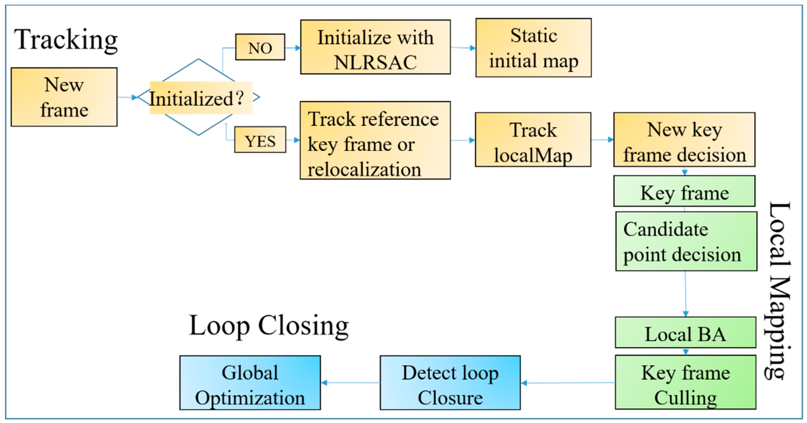
ORB-SLAM2 integrates modules such as map initialization, inter-frame estimation, local map management, and closed-loop detection, which provides good experimental comparison objects for subsequent research. So, we adapted ORB-SLAM2 to provide basic framework for creating a static map and robustly estimating camera pose. Among them, the closed loop process in the system is identical to ORB-SLAM2. Figure 1 shows the framework of DM-SLAM. DLRSAC is integrated into initialization in the tracking thread to construct an original map. Also, the expansion rules of the map are designed to weaken the effects of dynamic objects in the mapping thread. Below, we describe the measures that have been taken to improve the robustness of system motion when compared to ORB-SLAM2.
2.3.1. DLRSAC Implementation in DM-SLAM
DLRSAC performs static semantic extraction to create a static initial map with respect to ORB-SLAM2. This algorithm doesn’t require any prior information, yet it introduces distribution degree evaluation to break the problem of “chicken-egg” circulation in dynamic scenes. The camera pose estimation can be completed more confidentially and more accurately even if static feature points in the scene don’t take precedence.
Static initial maps are constantly used in camera tracking, which affect subsequent map expansion. Therefore, the accuracy of DLRSAC is much more important than the recall rate. The accuracy of the algorithm is improved by analyzing the reason why the algorithm fails, introducing detection methods and resetting the system when failure occurs. Analysis of the reasons for failure is reviewed below:
- The parallax between the two frames is so small that solving F matrix at this time is pathological problem.
- The motion in the scene is too complicated to affect the model selection in each grid, so the motion model is finally selected.
- The scene appears motion blur (low-textured area), leading to few matches and few sufficient Grid models.
Detection methods are reviewed below:
- Verify the parallax of map points. If the mean value is too small, the algorithm is considered to fail. In order to call a large parallax, we use two frames separated by several frames instead of two consecutive frames at the time of initialization. An additional benefit of doing this is that it makes the motion and noise separable.
- Verify that the distribution of selected Grid model. If the value is too small, the algorithm is considered to fail.
- Check the two frames used for initialization, reset system if there are too few features matching.
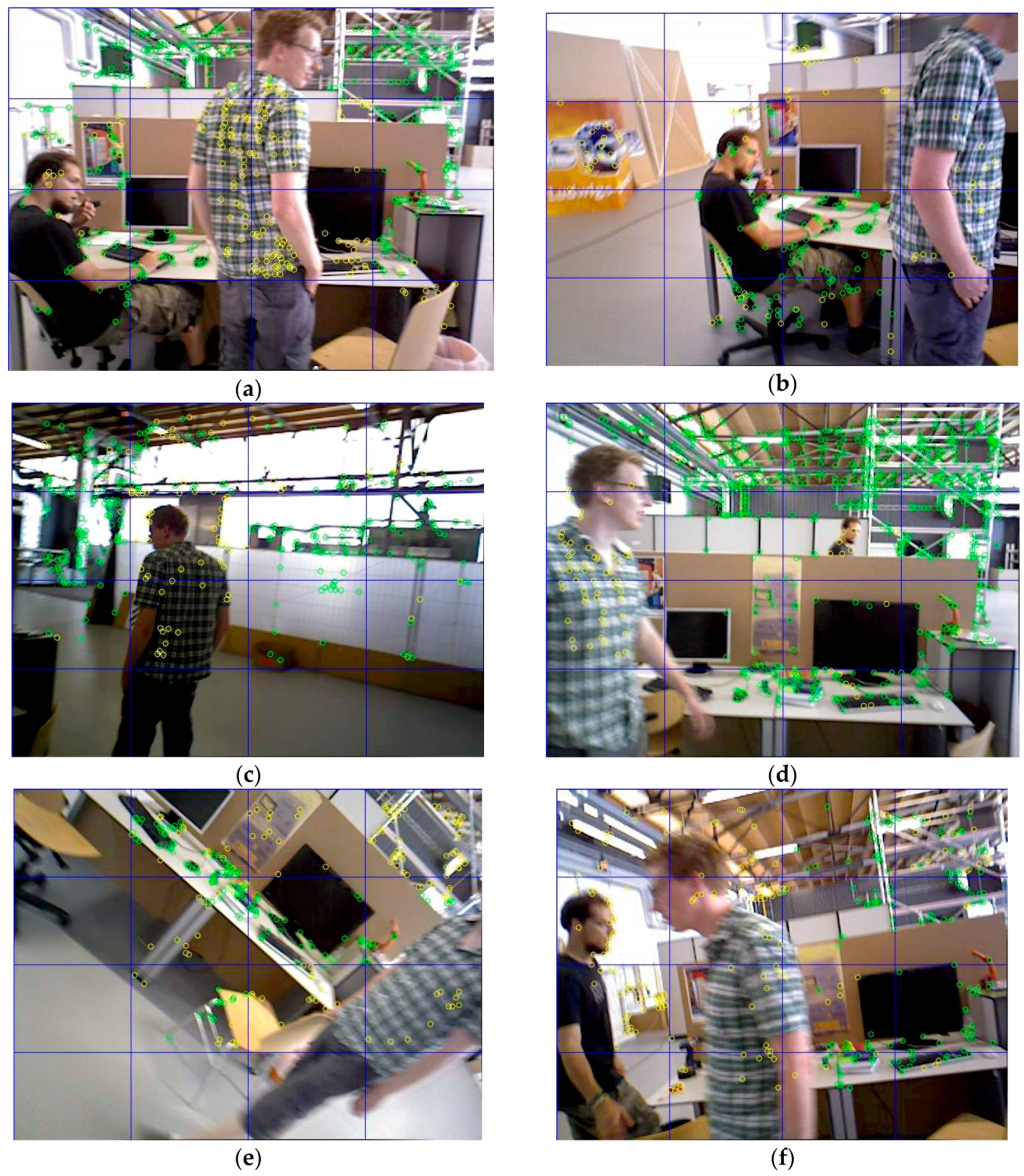
We delay the initialization until this method passes the failure test. Figure 2 shows the static feature extraction effect of the algorithm in different motion scenarios in TUM fr3_walking_rpy.
2.3.2. Tracking Thread
In tracking thread of other visual SLAM systems, the motion model [16] is usually used to initialize camera pose, and then outliers are eliminated in subsequent optimizations. First we track the matching features between current frame and current reference key frame, estimate the camera’s initial pose, then track the local map to get more feature matches. Finally, camera pose optimization is performed. This approach essentially is a method of reconstruction after segmentation. Dynamic objects are able to be managed because the definition of the static map has been implemented in the initialization. See ORB-SLAM2 [16] for details on local map.
3. Results
In order to show the effectiveness of the DLRSAC algorithm in more detail, we not only run DM-SLAM on a public data set, but also perform DLRSAC experiments. Experiments are tested in dynamic environments within the public TUM RGB-D dataset [17] while depth images are ignored. High dynamic fr3_walking sequences are typically very challenging because people walking in the scene increases the difficulty of monocular SLAM. First, we show the static features extraction results of initialization using DLRSAC in different scenarios of fr3_walking_rpy sequence after tacking fails, as well as intermediate results in the tracking. Then, we test the time required by the DLRSAC algorithm and compared it with RANSAC and ARSAC. Finally, we evaluate the performance of DM-SLAM in some sequences of TUM-RGB-D dataset. All experiments are performed on a computer with Intel i7 CPU, and 8GB RAM.
3.1. Evaluations of DLRSAC
Unlike the data used in comparison of algorithms [9] like RANSAC, LoSAC [18], Multi-GS [19] and ARSAC [9], where the dynamic objects change significantly in geometry, the data used in the operation of this system is quite different. In our experiments, we used successive frames in video sequences, including our own data and TUM sequence fr3_walking_rpy.
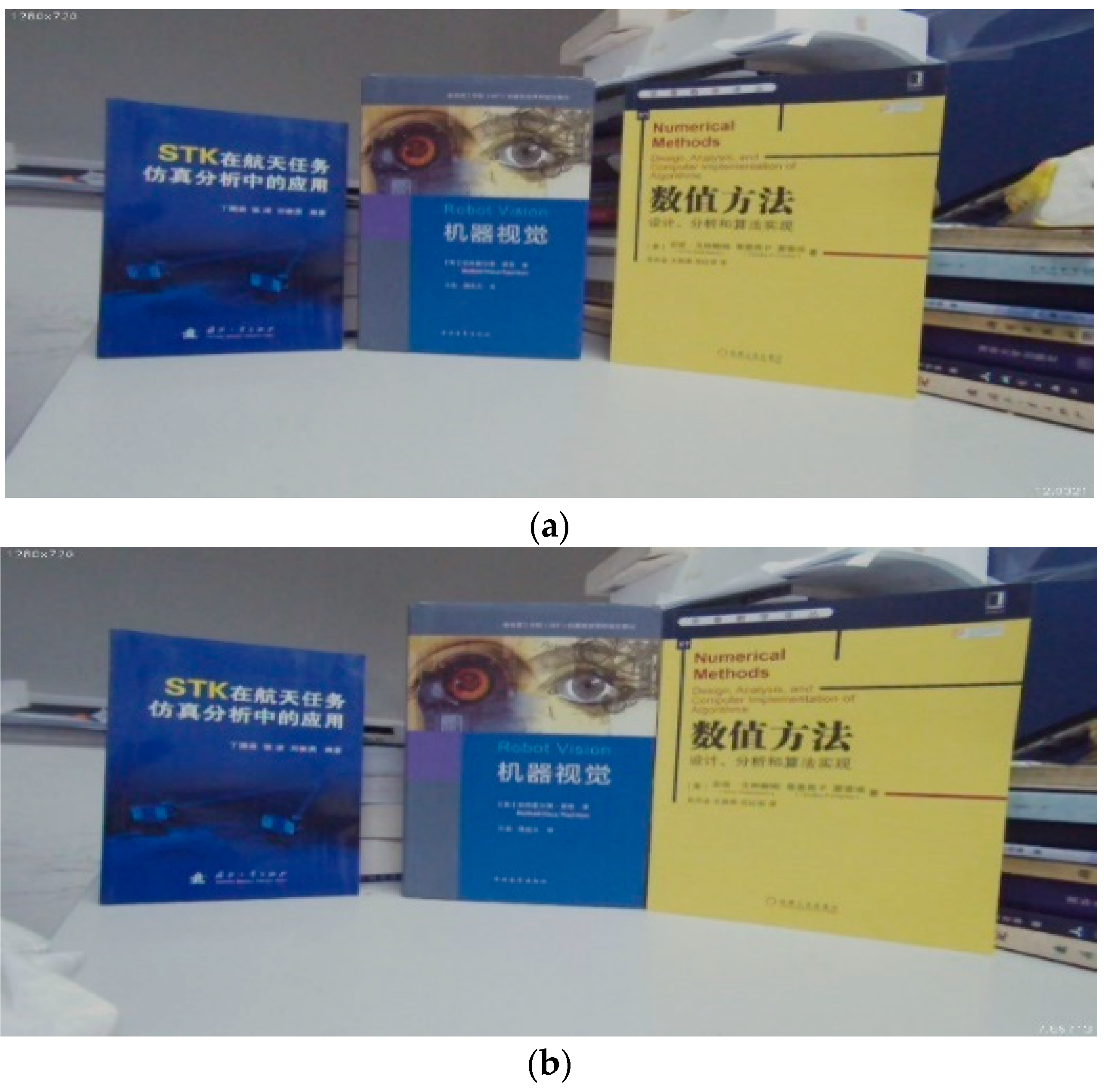
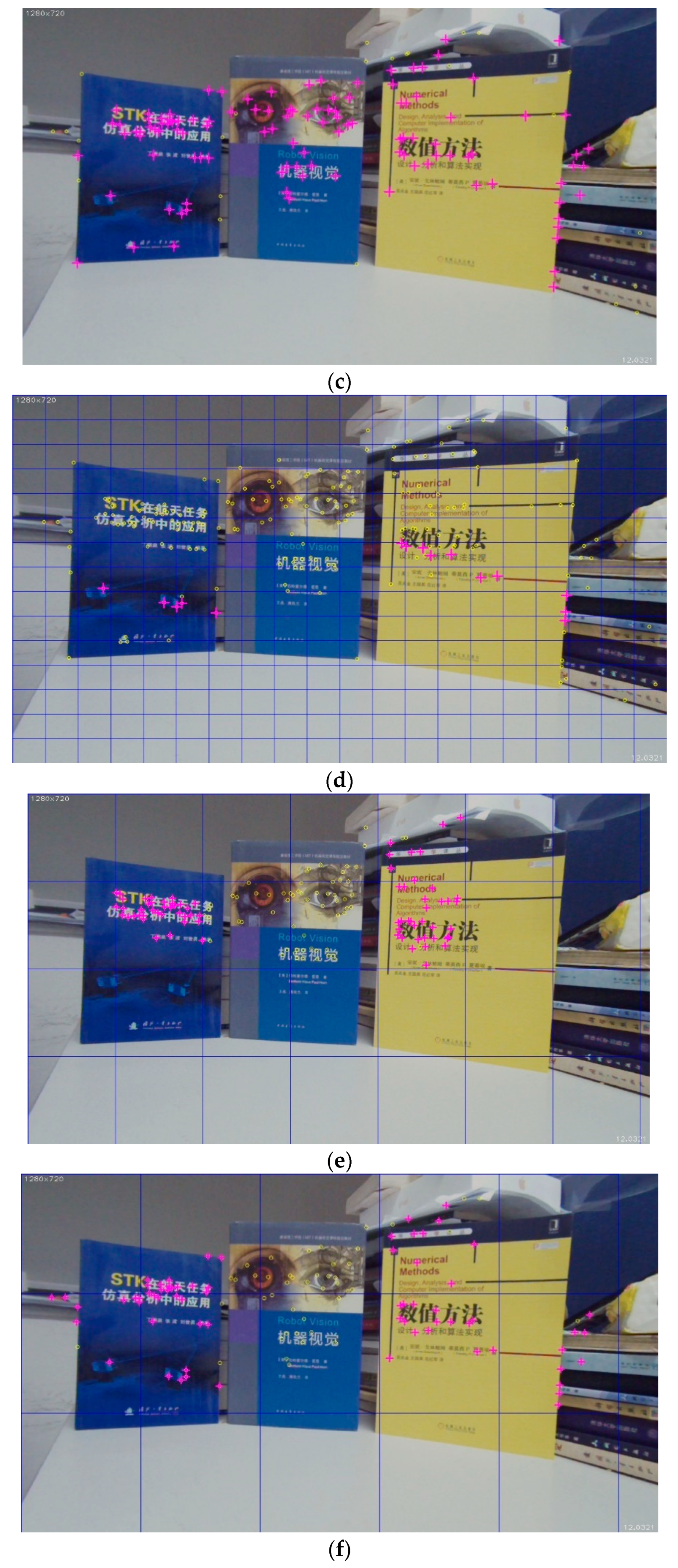
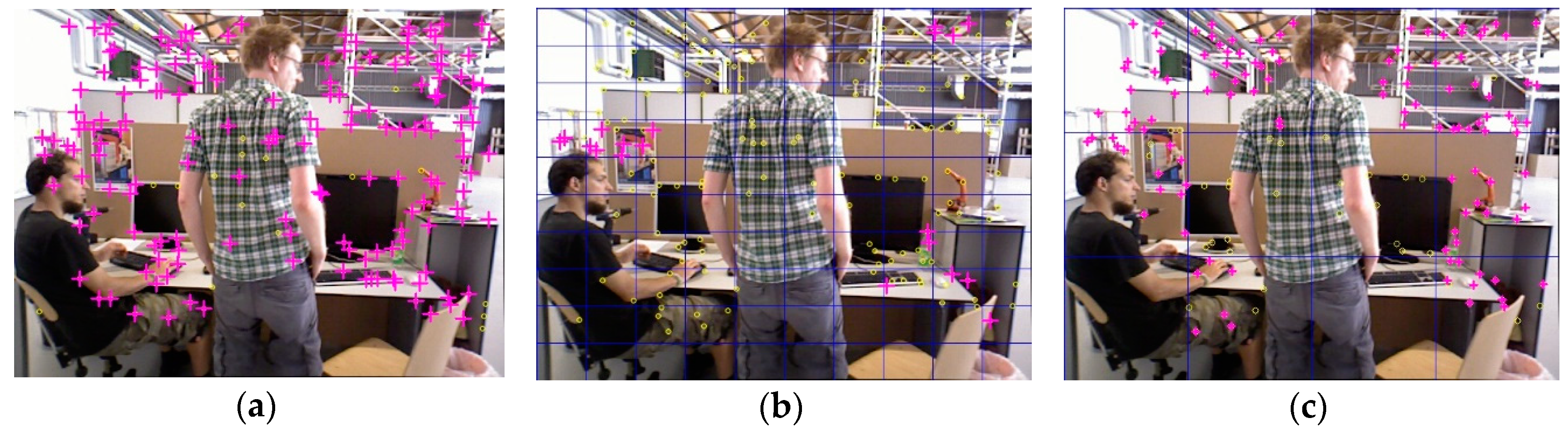
Figure 3 displays results tested in our data, where the middle book in the source images is moving. Our data is used to compare algorithms where there are rigid-body motions in the scene. Figure 4 shows the results tested in TUM fr3_walking_rpy, which verify the performance of algorithms when there are non-rigid objects in the scene. We compared our algorithm with others, including standard RANSAC [8] and ARSAC [9]. We choose ARSAC instead of PARSAC because obtaining prior information of the inliers ratio in the images is not practical. As can be seen in Figure 4e–f, most static features can be extracted with DLRSAC, with the exception of static features in the conditions below:
- The feature is so independent from other features that the number of feature points in the local grid does not satisfy the solution condition.
- Some static features belong to the grid in which moving features dominate, meaning that the grid is not classified into the Coupled Grid set (so all features in the grid are considered as moving features).
We can see from Figure 3c and Figure 4a that RANSAC has almost no distinguishing ability for moving objects in consecutive frames. And, although ARSAC can extract a part of static features, like Figure 3d and Figure 4b, the extracted features are much lower in number than those of DLRSAC. We hypothesize that this is because ARSAC only takes the degree of distribution as the objective function optimization variable.
In addition, the computational overhead of DLRSAC is slightly longer than RANSAC and ARSAC while within acceptable circumstances, as listed in Table 1 (the iteration number is set to 2000).
The purpose of dividing an image into grids is to reduce the complexity of motion within the grid so that the points that are sampled to solve the Grid model are more likely to belong to the same motion model. As we know, under RANSAC taken to solve Grid model, the number of iterations required to guarantee a correct solution is:
where s is the number of data points, ε is the percentage of outliers, and p is the probability of success (confidence level) [20]. In fact, RANSAC tends to choose models that are solved by features from multiple source models, as shown in Figure 3. These models have stronger Coupling ability in local grid but less in global image, which helps DLRSAC filter out real static features. Aside from this, we find that the selected model has stabilized after several hundred iterations due to this nature. The grid selected in Figure 5 contains a moving person and surrounding static environments, where red circles are the selected eight initial points used to solve the solution model. The eight points are from both moving and static objects, but almost all the points in the grid are their inliers.
3.2. Initialization and Tracking Performance
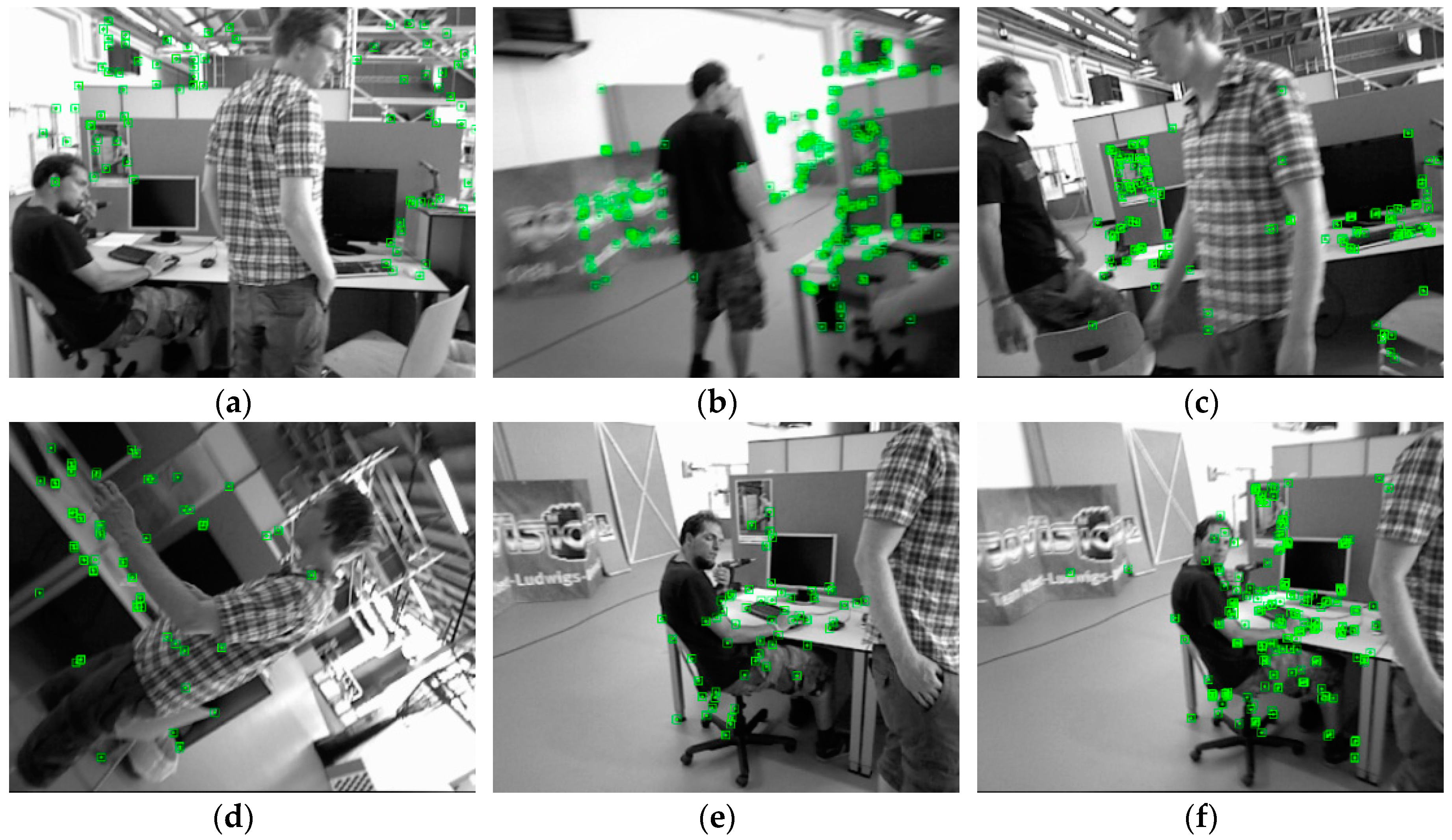
In sequence fr3_walking, there are two men walking around the desk. The men are the only movable objects, which causes a highly dynamic scene. Sequence fr3_walking includes rpy, xyz, and half sphere, which stands for three types of camera ego-motions. Sequence fr3_walking_rpy indicates that rotation is dominant in camera movement, sequence fr3_walking_xyz indicates that translation is dominant in camera movement, and sequence fr3_walking_half_sphere indicates that both camera motion and rotation are obvious. In order to verify the performance of DLRSAC in different motion scenarios, we randomly tested our algorithm in different frames in the fr3_walking sequence, and then selected several typical motion scenes to show performance of static features extraction of our algorithm. The results are shown in Figure 6. In Figure 6e–f, although there is certain motion blur in the environment, the algorithm still extracts most of the static features.
It can be seen that DM-SLAM removes most motion features during the tracking process. In the map expansion, although motion features are added to the map points occasionally, the limitation on the distribution and number of newly added map points weakened the influence of new added points on the camera pose calculation. In turn, the correct camera pose assures the geometric constraint relationship, which allows the system to eliminate motion features based on the projection error of the newly added map points in subsequent frames.
3.3. Overall Evaluation Using TUM RGB-D Dataset
It is worth noting that the determination of static objects in the DM-SLAM system stems from the solution of the model in the grid. Therefore, DM-SLAM is not suitable for the situation where massive moving objects exist in the scene, resulting in the static background blocked in various parts of images. The most scenes in TUM RGB-D dataset are indoor and the motion situation is not too complicated. At the same time, sequence fr3_walking includes many different types of camera motions, such as rpy, xyz, and half_sphere, where we can observe the performance of the SLAM system more comprehensively. Therefore, we chose TUM sequence fr3_walking to compare ORB-SLAM2 with DM-SLAM. Table 2, Table 3 and Table 4 show quantitative comparison results of ORB-SLAM2 and DM-SLAM in sequences fr3_walking and fr1_xyz. As Berta, B and Facil, J proposed in [1], we run each sequence ten times and show RMSE (RootMeanSquareError), mean, media, S.D. results, to account for non-deterministic nature of the system. In order to compare the basic performance of DRLRSAC, we have added alignment with sequence fr1_xyz, which is dominated by static scenes. RMSE, Mean Error, Median Error, and Standard Deviation (S.D.) indicates SLAM errors from different aspects, but RMSE and S.D. are more relevant because they can better indicate the robustness and stability of the system. The calculation method of improvements refers to literature [17].
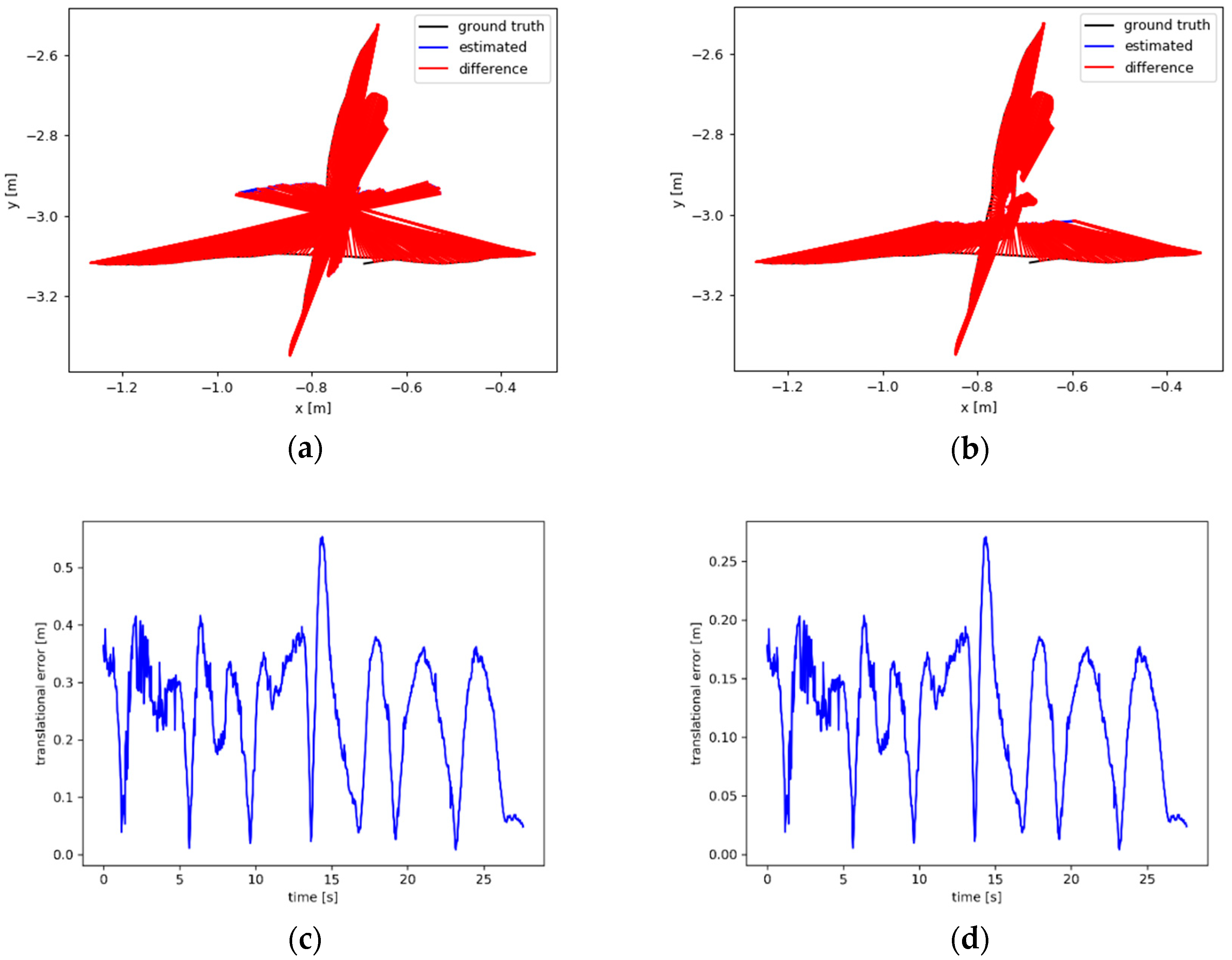
As we can see from Table 2, Table 3 and Table 4 there is obvious improvement when compared DM-SLAM with ORB-SLAM2. In sequence fr3_walking, the RMSE and S.D. improvement values of ATE can reach up to 96.42% and 98.45%. DM-SLAM errors are mainly caused by outliers, mismatches, and numerical calculations. We think that improvement depends on the ratio between the errors caused by the moving object and the above errors. In fr1_xyz, the improvement in performance is not obvious and we hypothesized that when the scene is mainly static, the distinction of DM-SLAM for dynamic features is not necessary for ORB-SLAM2 system.
Figure 7 shows the ATE and results of metric rotational drift (RPE) from ORB-SLAM2 and DM-SLAM respectively. It can be seen that the overall error of DM-SLAM is much smaller than ORB-SLAM2. In experiments, when the number of feature points extracted per frame (default) is 1000, ORB-SLAM2 cannot work (while DM-SLAM works). For comparison, we set the number of feature points extracted per frame 3000, which improves the data association between frames and robustness of the system.
4. Conclusions
In this paper, we propose a DM-SLAM system based on ORB-SLAM2 to adapt to dynamic environments. DLRSAC is proposed to extract the most static matches for initialization even when dynamic objects take dominate whether dynamic objects are non-rigid or rigid. In regard to tracking thread, we designed a neighborhood mutual exclusion algorithm to limit the number of candidate maps. This algorithm reduces the interference of dynamic features on camera tracking and ensures rapid expansion of the map. Due to the above techniques, DM-SLAM system can successfully operate in a dynamic environment even when moving objects dominate the scene.
The limitation of this method is that when a large number of stationary objects appear in the scene and then move in the tracking process, the algorithm will fail. Because in this case the static objects essentially represent the reference coordinate system, the motion of the reference coordinate system cannot be detected in this algorithm.
In our observation, static means the most suitable reference coordinate system in the whole world. In under-textured areas, non-feature pixels can be used to find the global optimal reference coordinate system, which is beyond feature-based methods. In the future, we are considering introducing a direct method to extend the ability of DM-SLAM to adapt to richer dynamic scenarios.
Author Contributions
Conceptualization, X.L. and S.T.; Data curation, X.L. and H.H.; Formal analysis, X.L.; Funding acquisition, H.W.; Methodology, X.L.; Project administration, S.T.; Resources, X.L. and S.T.; Software, X.L.; Supervision, S.T. and C.L.; Validation, C.L. All authors have read and agreed to the published version of the manuscript.
Funding
This work is supported by the National Key R&D Program of China (No.2017YFB1002800); Beijing Natural Science Foundation (No. 8172018) and the National Key Research and Development Program (No. 2018YFB1601003).
Conflicts of Interest
The authors declare no conflict of interest. The funders had no role in the design of the study; in the collection, analyses, or interpretation of data; in the writing of the manuscript, or in the decision to publish the results.
References
- Berta, B.; Facil, J.M.; Javier, C. DynaSLAM: Tracking, Mapping and Inpainting in Dynamic Scenes. IEEE Robot. Autom. Lett. 2018, 3, 4076–4083. [Google Scholar]
- Mur-Artal, R.; Tardós, J.D. Orb-slam2: An open-source slam system for monocular, stereo, and rgb-d cameras. IEEE Trans. Robot. 2017, 33, 1255–1262. [Google Scholar] [CrossRef] [Green Version]
- Engel, J.; Schöps, T.; Cremers, D. LSD-SLAM: Large-scale direct monocular SLAM. In Proceedings of the European Conference on Computer Vision; Springer: Cham, Switzerland, 2014; pp. 834–849. [Google Scholar]
- Engel, J.; Koltun, V.; Cremers, D. Direct sparse odometry. IEEE Trans. Pattern Anal. Mach. Intell. 2017, 40, 611–625. [Google Scholar] [CrossRef] [PubMed]
- Engel, J.; Sturm, J.; Cremers, D. Semi-Dense Visual Odometry for a Monocular Camera. In Proceedings of the IEEE International Conference on Computer Vision, Sydney, Australia, 1–8 December 2013; pp. 1449–1456. [Google Scholar]
- Forster, C.; Pizzoli, M.; Scaramuzza., D. SVO: Fast semi-direct monocular visual odometry. In Proceedings of the 2014 IEEE International Conference on Robotics and Automation (ICRA), Hong Kong, China, 31 May–7 June 2014; IEEE: Piscataway, NJ, USA, 2014; pp. 15–22. [Google Scholar]
- Fischler, M.A.; Bolles, R.C. Random sample consensus: A paradigm for model fitting with applications to image analysis and automated cartography. Commun. ACM 1981, 24, 381–395. [Google Scholar] [CrossRef]
- Saputra, M.R.U.; Markham, A.; Trigoni, N. Visual SLAM and structure from motion in dynamic environments: A survey. ACM Comput. Surv. 2018, 51, 1–37. [Google Scholar] [CrossRef]
- Tan, W.; Liu, H.; Dong, Z. Robust monocular SLAM in dynamic environments. In Proceedings of the 2013 IEEE International Symposium on Mixed and Augmented Reality (ISMAR), Adelaide, SA, Australia, 1–4 October 2013; pp. 209–218. [Google Scholar]
- Sun, Y.; Liu, M.; Meng, M.Q.H. Improving rgb-d slam in dynamic environments: A motion removal approach. Robot. Auton. Syst. 2017, 89, 110–122. [Google Scholar] [CrossRef]
- Kitt, B.; Moosmann, F.; Stiller, C. Moving on to dynamic environments: Visual odometry using feature classification. In Proceedings of the 2010 IEEE/RSJ International Conference on Intelligent Robots and Systems, Taipei, Taiwan, 18–22 October 2010; IEEE: Piscataway, NJ, USA, 2010; pp. 5551–5556. [Google Scholar]
- Chao, Y.; Zuxin, L.; Xinjun, L. DS-SLAM: A Semantic Visual SLAM towards Dynamic Environments. In Proceedings of the 2018 IEEE/RSJ International Conference on Intelligent Robots and Systems (IROS), Madrid, Spain, 1–5 October 2018; IEEE: Piscataway, NJ, USA, 2018. [Google Scholar]
- Schindler, K.; James, U.; Wang, H. Perspective n-view multibody structure-and-motion through model selection. In Proceedings of the European Conference on Computer Vision; Springer: Berlin/Heidelberg, Germany, 2006; pp. 606–619. [Google Scholar]
- Vidal, R.; Ma, Y.; Sastry, S. Generalized principal component analysis. IEEE Trans. Pattern Anal. Mach. Intell. 2005, 27, 1945–1959. [Google Scholar] [CrossRef] [PubMed] [Green Version]
- Yan, J.; Pollefeys, M. A general framework for motion segmentation: Independent, articulated, rigid, non-rigid, degenerate and non-degenerate. In Proceedings of the European Conference on Computer Vision; Springer: Berlin/Heidelberg, Germany, 2006; pp. 94–106. [Google Scholar]
- Mur-Artal, R.; Montiel, J.M.M.; Tardos, J.D. ORB-SLAM: A versatile and accurate monocular SLAM system. IEEE Trans. Robot. 2015, 31, 1147–1163. [Google Scholar] [CrossRef] [Green Version]
- Sturm, J.; Engelhard, N. A benchmark for the evaluation of RGB-D SLAM systems. In Proceedings of the 2012 IEEE/RSJ International Conference on Intelligent Robots and Systems, Vilamoura, Portugal, 7–12 October 2012; IEEE: Piscataway, NJ, USA, 2012. [Google Scholar]
- Chum, O.; Matas, J.; Kittler, J. Locally optimized RANSAC. In Proceedings of the Joint Pattern Recognition Symposium; Springer: Berlin/Heidelberg, Germany, 2003; pp. 236–243. [Google Scholar]
- Chin, T.J.; Yu, J.; Suter, D. Accelerated hypothesis generation for multistructure data via preference analysis. IEEE Trans. Pattern Anal. Mach. Intell. 2011, 34, 625–638. [Google Scholar] [CrossRef] [PubMed]
- Fuentes-Pacheco, J.; Ruiz-Ascencio, J.; Rendón-Mancha, J.M. Visual simultaneous localization and mapping: A survey. Artif. Intell. Rev. 2015, 43, 55–81. [Google Scholar] [CrossRef]
Figure 1.
The framework of DM-SLAM. DM-SLAM share same loop closing thread with ORB-SLAM2. There are three process including tracking, local mapping and loop closing. Tracking is mainly responsible for extracting the initial pose of the camera utilizing the input images, where we integrate distribution and local-based RANSAC algorithm (DLRSAC) into the initialization in tracking process. Local mapping is responsible for saving, filtering and optimizing key frames and map points, where we integrate algorithms 1 into candidate point decision. The closed-loop detection mainly detects whether there is a closed-loop, and if so, global optimization is performed.

Figure 2.
Static features extraction results of different frames in sequence fr3_walking_rpy. Inliers are marked with green circle, while yellow circles are considered to be outliers. (a–f) depicts the movement scene at different moments in TUM fr3_walking_rpy.
Figure 2.
Static features extraction results of different frames in sequence fr3_walking_rpy. Inliers are marked with green circle, while yellow circles are considered to be outliers. (a–f) depicts the movement scene at different moments in TUM fr3_walking_rpy.

Figure 3.
Real example for static extraction. (a) and (b) are source images, which show that the book in the middle is moving. (c) The static points recognized by RANSAC, marked with red crosses. The outliers are marked with yellow circles. (d) The static points recognized by ARSAC [16]. (e) The static points recognized by our DLRSAC with the size of grid is 180 × 180. (f) The static points recognized by our DLRSAC with the size of grid is 240 × 240.


Figure 4.
Samples in TUM sequence fr3_walking_rpy. As seen in Figure 3, static points are marked with green circles while others are marked with yellow circles. (a) Recognition results by RANSAC. (b) Recognition results by ARSAC. (c) Recognition results by DLRSAC.
Figure 4.
Samples in TUM sequence fr3_walking_rpy. As seen in Figure 3, static points are marked with green circles while others are marked with yellow circles. (a) Recognition results by RANSAC. (b) Recognition results by ARSAC. (c) Recognition results by DLRSAC.

Figure 5.
Solution result in grids containing mixed model. Red circles: eight features solving Grid model, blue circles: all matching feature points, and yellow circles: inliers of the Grid model.
Figure 5.
Solution result in grids containing mixed model. Red circles: eight features solving Grid model, blue circles: all matching feature points, and yellow circles: inliers of the Grid model.

Figure 6.
The features used for solving camera pose in the tracking thread, which are marked with green circle. (a–f) show performance of static features extraction of our algorithm in several typical motion scenes.
Figure 6.
The features used for solving camera pose in the tracking thread, which are marked with green circle. (a–f) show performance of static features extraction of our algorithm in several typical motion scenes.

Figure 7.
(a) and (c) are ATE and RPE from ORB-SLAM2 respectively. (b) and (d) are ATE and results of metric rotational drift (RPE) from DM-SLAM, respectively.
Figure 7.
(a) and (c) are ATE and RPE from ORB-SLAM2 respectively. (b) and (d) are ATE and results of metric rotational drift (RPE) from DM-SLAM, respectively.


Table 1.
The average running time of different algorithms.
| Algorithm | RANSAC | ARSAC | DLRSAC |
|---|---|---|---|
| Running time | 34.6 ms | 36.8 ms | 40.1 ms |
| Iterations | 2000 | 2000 | 2000 |
Table 2.
Results of metric rotational drift (RPE).
| Sequences. | ORB-SLAM2 | DM-SLAM | Improvements | |||||||||
|---|---|---|---|---|---|---|---|---|---|---|---|---|
| RMSE | MEAN | MEDIAN | S.D. | RMSE | MEAN | MEDIAN | S.D. | RMSE | MEAN | S.D. | RMSE | |
| fr3_walking_xyz | 2.4385 | 1.5697 | 0.9472 | 1.8661 | 0.6012 | 0.5143 | 0.4302 | 0.3109 | 75.30% | 67.20% | 54.50% | 83.30% |
| fr3_walking_rpy | 3.3087 | 2.8813 | 2.9891 | 1.6265 | 0.9222 | 0.8085 | 0.7763 | 0.4436 | 75.12% | 77.20% | 74.02% | 72.72% |
| fr3_walking_half | 3.6495 | 3.8041 | 3.1594 | 1.8542 | 1.2591 | 1.1187 | 1.0663 | 0.5775 | 65.49% | 64.47% | 66.24% | 68.85% |
| fr1_xyz | 1.0088 | 0.8911 | 0.8717 | 0.4728 | 0.8372 | 0.7371 | 0.6657 | 0.3969 | 17.01% | 17.28% | 17.63% | 16.05% |
Table 3.
Results of metric translational drift (RTE).
| Sequences | ORB-SLAM2 | DM-SLAM | Improvements | |||||||||
|---|---|---|---|---|---|---|---|---|---|---|---|---|
| RMSE | MEAN | MEDIAN | S.D. | RMSE | MEAN | MEDIAN | S.D. | RMSE | MEAN | S.D. | RMSE | |
| fr3_walking_xyz | 0.4888 | 0.4352 | 0.4687 | 0.2224 | 0.2803 | 0.2643 | 0.2643 | 0.0931 | 42.65% | 42.46% | 43.46% | 58.13% |
| fr3_walking_rpy | 0.4221 | 0.3862 | 0.3955 | 0.2266 | 0.1671 | 0.1405 | 0.1683 | 0.0901 | 60.41% | 63.62% | 57.44% | 60.24% |
| fr3_walking_half | 0.7241 | 0.6307 | 0.6437 | 0.3557 | 0.3852 | 0.3251 | 0.3511 | 0.1341 | 46.94% | 48.45% | 45.45% | 57.53% |
| fr1_xyz | 0.0705 | 0.0606 | 0.0643 | 0.0343 | 0.0438 | 0.0401 | 0.0427 | 0.0186 | 37.59% | 33.82% | 21.61% | 45.77% |
Table 4.
Results of metrics absolute trajectory error (ATE).
| Sequences | ORB-SLAM2 | DM-SLAM | Improvements | |||||||||
|---|---|---|---|---|---|---|---|---|---|---|---|---|
| RMSE | MEAN | MEDIAN | S.D. | RMSE | MEAN | MEDIAN | S.D. | RMSE | MEAN | S.D. | RMSE | |
| fr3_walking_xyz | 0.3292 | 0.3078 | 0.2942 | 0.1161 | 0.1429 | 0.1298 | 0.1352 | 0.0537 | 56.59% | 57.83% | 54.04% | 53.74% |
| fr3_walking_rpy | 2.9432 | 2.7549 | 2.8641 | 1.8461 | 0.1055 | 0.1016 | 0.0864 | 0.0285 | 96.42% | 96.31% | 96.98% | 98.45% |
| fr3_walking_half | 0.5121 | 0.4534 | 0.3867 | 0.2379 | 0.1548 | 0.1254 | 0.1481 | 0.0716 | 69.77% | 72.34% | 61.71% | 69.91% |
| fr1_xyz | 0.0492 | 0.0467 | 0.0439 | 0.0151 | 0.0285 | 0.0271 | 0.0277 | 0.0086 | 42.01% | 41.97% | 36.91% | 43.05% |
© 2020 by the authors. Licensee MDPI, Basel, Switzerland. This article is an open access article distributed under the terms and conditions of the Creative Commons Attribution (CC BY) license (http://creativecommons.org/licenses/by/4.0/).
Share and Cite
MDPI and ACS Style
Lu, X.; Wang, H.; Tang, S.; Huang, H.; Li, C. DM-SLAM: Monocular SLAM in Dynamic Environments. Appl. Sci. 2020, 10, 4252. https://0-doi-org.brum.beds.ac.uk/10.3390/app10124252
AMA Style
Lu X, Wang H, Tang S, Huang H, Li C. DM-SLAM: Monocular SLAM in Dynamic Environments. Applied Sciences. 2020; 10(12):4252. https://0-doi-org.brum.beds.ac.uk/10.3390/app10124252
Chicago/Turabian StyleLu, Xiaoyun, Hu Wang, Shuming Tang, Huimin Huang, and Chuang Li. 2020. "DM-SLAM: Monocular SLAM in Dynamic Environments" Applied Sciences 10, no. 12: 4252. https://0-doi-org.brum.beds.ac.uk/10.3390/app10124252
Note that from the first issue of 2016, this journal uses article numbers instead of page numbers. See further details here.