
Automatic Identification of Peanut-Leaf Diseases Based on Stack Ensemble

1
College of Engineering, South China Agricultural University, Guangzhou 510642, China
2
Center for International Collaboration Research on Precision Agricultural Aviation Pesticides, Spraying Technology (NPAAC), South China Agricultural University, Guangzhou 510642, China
3
Guangdong Laboratory for LingNan Modern Agriculture, Guangzhou 510642, China
4
Department of Electrical & Computer Engineering, College of Engineering, University of Washington, Seattle, WA 98195-2500, USA
*
Author to whom correspondence should be addressed.
Appl. Sci. 2021, 11(4), 1950; https://0-doi-org.brum.beds.ac.uk/10.3390/app11041950
Submission received: 26 January 2021
/
Revised: 10 February 2021
/
Accepted: 19 February 2021
/
Published: 23 February 2021
(This article belongs to the Section Food Science and Technology)
Abstract
:Peanut is an important food crop, and diseases of its leaves can directly reduce its yield and quality. In order to solve the problem of automatic identification of peanut-leaf diseases, this paper uses a traditional machine-learning method to ensemble the output of a deep learning model to identify diseases of peanut leaves. The identification of peanut-leaf diseases included healthy leaves, rust disease on a single leaf, leaf-spot disease on a single leaf, scorch disease on a single leaf, and both rust disease and scorch disease on a single leaf. Three types of data-augmentation methods were used: image flipping, rotation, and scaling. In this experiment, the deep-learning model had a higher accuracy than the traditional machine-learning methods. Moreover, the deep-learning model achieved better performance when using data augmentation and a stacking ensemble. After ensemble by logistic regression, the accuracy of residual network with 50 layers (ResNet50) was as high as 97.59%, and the F1 score of dense convolutional network with 121 layers (DenseNet121) was as high as 90.50. The deep-learning model used in this experiment had the greatest improvement in F1 score after the logistic regression ensemble. Deep-learning networks with deeper network layers like ResNet50 and DenseNet121 performed better in this experiment. This study can provide a reference for the identification of peanut-leaf diseases.
1. Introduction
Peanut is a crop with multiple uses and a very rich nutritional value. As the main oil and economic crop in the Guangdong Province of China, its growing area is constantly increasing, and it has become the second-largest cultivated crop in Guangdong Province [1]. The peanut itself and the complex field environment make the leaves easy to be infected by pathogens. The pathogen can spread rapidly through natural factors and has a high reproductive capacity. The main factor affecting its reproduction is the humidity of peanuts during the seedling stage [2]. Diseases of peanut leaves can reduce the yield and quality of peanuts by destroying the green tissue and chlorophyll in the leaves [3]. Artificial identification of peanut-leaf diseases requires professional knowledge, and it is easy to misdiagnose them only by artificial visual observation. In this way, peanut diseases cannot be diagnosed and treated in time. The key to control peanut disease is to diagnose the disease type quickly and accurately, and then take corresponding control measures in time.
With the development of computer technology, traditional machine-learning methods have been successfully applied to many fields. Beltran-Perez combined a multiscale generalized radial basis function network with discrete cosine transform, and successfully applied this method to a computer-aided diagnosis system for breast-cancer detection [4]. For fire sensitivity prediction and mapping, Pham evaluated four machine-learning methods. The models were evaluated using the area under the receiver operating characteristic curve and seven other performance metrics. The results showed that these models were sufficiently robust in responding to the training and verification dataset changes [5]. In terms of urban planning, Nikola successfully used a machine-learning method to classify the green infrastructure of satellite images [6]. In recent years, random forest, k-means, and support vector machine [7,8,9] algorithms based on traditional machine learning have been applied to plant-disease diagnosis. Wang et al. used a vector median filter to remove noise from collected corn-disease color pictures, then extracted the texture and color features of the corn-disease image as feature vectors, and then mapped the input space samples to high-dimensional space features for K-means clustering and plant-disease identification, and the final identification rate of their four corn diseases was 82.5% [10]. Es-saady et al. proposed a technology based on the serialization of two support vector machine classifiers, with one classifier extracting the color features of the picture, and the other classifier distinguishing the classes of similar colors according to the shape and texture features, and the accuracy rate reached 87.80% [11]. Moheson et al. used hyperspectral data to identify wheat leaf rust. Four machine-learning methods, including v-support vector regression, enhanced regression tree, random forest regression and Gaussian process regression, were established to estimate the severity of rust at the canopy scale. The experiment showed that hyperspectral signatures could be used in the identification of wheat leaf rust at different leaf area index levels [12]. Tan et al. performed background cutting on soybean leaf pictures, determined the chromaticity value of the leaves, and established several layers of back-propagation neural networks. The accuracy of the soybean disease spot-recognition rate was 92.1% [13]. Wang et al. proposed a method of plant-disease recognition that extracted 21 color features, 25 texture features and 4 shape features from the images of diseased leaves of wheat and grape, processed the features with principal component analysis (PCA), and classified wheat and grape diseases with multiple neural-network classifiers. The results showed that the PCA neural-network-based image recognition was the best method to detect and diagnose plant-leaf diseases [14].
In recent years, deep-learning methods have led a revolution in many fields such as speech recognition [15,16], object detection [17,18], and pose estimation [19,20]. Deep learning is a promising method for the automatic identification of plant diseases. By taking advantage of the sparse interaction, parameter sharing, and variable representation of a convolution network, it can effectively reduce network parameters, save model storage requirements, and improve the statistical efficiency of the network. Deep-learning methods have made some progress in recent years in identifying plant diseases and pests. Geetharamani et al. proposed a nine-layer deep convolutional neural network plant-disease-recognition model. This model recognized 39 different diseases of different plants on the open source dataset PlantVillage, and reached a 96.46% classification accuracy [21]. Hang et al. used the VGG16 model, Inception module, SE module, and the model of the pool average to identify a total of 10 diseases of cherry, apple, and corn, with an accuracy rate of 91.7%, while greatly reducing training time and model parameters [22]. Zhang et al. proposed a global pooled dilated convolutional neural network. By combining dilated convolution and global pooling, cucumber-leaf diseases were identified. The results showed that the model could effectively identify cucumber-leaf diseases [23]. In order to train a deep-learning model with good performance, a large number of data are often needed as the training set. However, datasets are very expensive, and the annotation of large datasets is a difficult problem. In this context, semisupervised learning methods aim at discovering and propagating labels to unsupervised samples, such that their correct labeling can improve the classification performance. Using the images of soybean leaves and herbivorous pests taken by Unmanned Aerial Vehicle, Willian et al. classified the unlabeled training set with a semisupervised method. The training set was used to train a convolutional neural network using different training strategies. The experimental results showed that the accuracy reached 98.90% when using the InceptionV3 structure and a semisupervised method to train the soybean-leaf dataset [24].
The above methods have a high accuracy in plant-disease identification, indicating that traditional machine learning and deep learning are effective methods for identifying plant diseases. However, the above deep-learning methods are only aimed at identifying a certain plant or a variety of plant leaves for a certain disease. In actual field production, plant leaves are often infected by multiple pathogens. This experiment mainly focused on the identification of mixed diseases and single diseases on a single leaf of peanut. The types of identification were healthy leaves, rust disease, scorch disease, leaf-spot disease, and both rust disease and scorch disease at the same time. In addition, the above methods do not have a good combination of deep-learning methods and traditional machine-learning methods. To obtain better classification performance, our study used the deep-learning model as the base-model and the traditional machine-learning model as the meta-model, and then used the predicted data of the base-model as the input features of the meta-model. In this experiment, five convolutional neural network structures, AlexNet, VGG16, residual network with 50 layers (ResNet50), dense convolutional network with 121 layers (DenseNet121), and InceptionV3, were selected as the base-model according to the depth and width of convolutional networks. Three traditional machine-learning methods, random forest (RF), logistic regression (LR), and support vector machine (SVM) were selected as the meta-model according to different classification thoughts.
In the second part of this article, we will provide an introduction to the chosen deep-learning model and the traditional machine-learning model, and explain in detail the out-of-fold prediction strategy used by the stack ensemble in this experiment. The results of the model fitting in this study are presented in Section 3, and the discussion is presented in Section 4. Finally, Section 5 gives our conclusion and future research directions.
2. Materials and Methods
2.1. Experimental Data
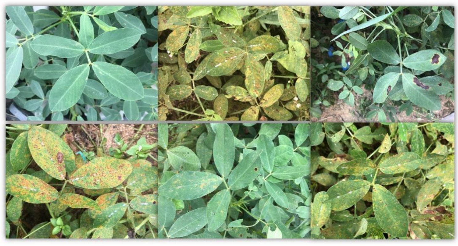
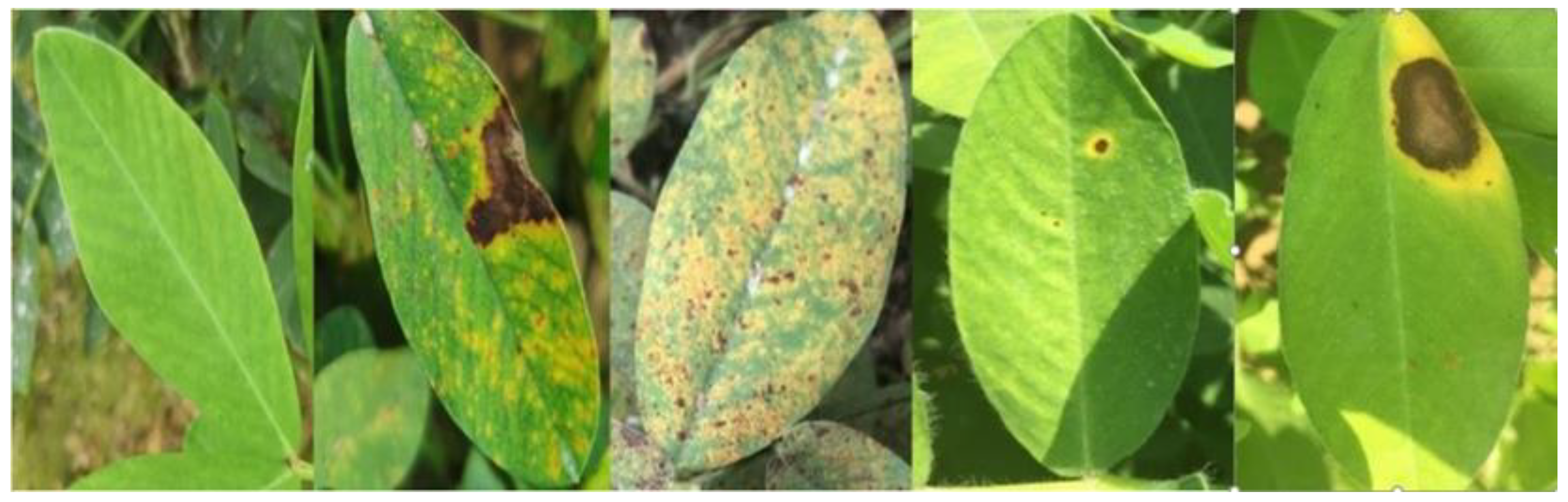
Diseased peanut leaves were collected manually at the agronomic experiment base of South China Agricultural University in Guangzhou City, Guangdong Province. A mobile phone was used as to take pictures (Figure 1). The original collection contained many diseased peanut leaves, and the classes of disease were different. Among the collected images, the parts of peanut leaves that were clear and the parts that showed disease spots were captured according to the size of the leaves using the screenshot tool (Figure 2). The captured images were sorted by disease class and used as the dataset for this study. The disease-image dataset included healthy leaves, scorch disease, leaf-spot disease, rust disease, and simultaneous rust disease and scorch disease. The total number of pictures taken with the mobile phone was about 2000. After cropping, we finally obtained 6029 pictures of peanut leaves, including 3205 of healthy leaves (HL), 463 of leaves with scorch disease (SD), 1359 of leaves with rust disease (RD), 346 of leaves with leaf-spot disease (LSD) and 656 of leaves suffering from both rust and scorch disease (RD + SD). The division ratio of the training set and the test set in this experiment was 4: 1 (Table 1) [25].
2.2. Deep Learning
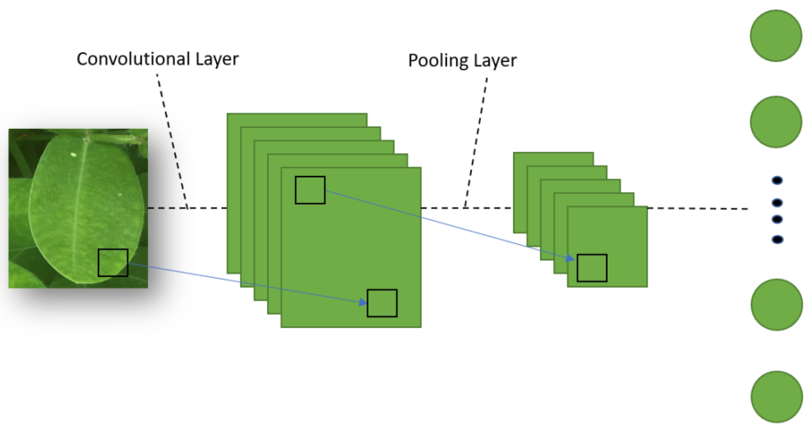
Deep learning is a very active field of computer vision and image classification. It builds a multilayer neural network, uses a large amount of label data, and obtains the feature representation of the data to improve the accuracy of classification or prediction. As shown in Figure 3, a typical deep convolutional network includes an input layer and an output layer or classifier, as well as many hidden layers [26]. The hidden layer includes a convolutional layer, a pooling layer, and some fully connected layers. Figure 3 shows a typical CNN (convolutional neural network) structure used by multiple network structures.
2.2.1. AlexNet
AlexNet was designed by Hinton, the winner of the 2012 ImageNet competition, and his student Alex Krizhevsky [27]. AlexNet uses an eight-layer neural network with five convolutional layers and three full-connectivity layers (three convolutional layers followed by a maximum pooling layer), and contains 630 million links, 60 million parameters, and 650,000 neurons. The successful use of a rectified linear unit (ReLU) as an activation function for CNN, which works better than Sigmoid in deeper networks, successfully solves the gradient diffusion problem of Sigmoid in deeper networks, and is a breakthrough in deep learning.
2.2.2. VGG
The VGG convolutional neural network is a model that was proposed by Oxford University in 2014 [28]. When this model was proposed, it immediately became a very popular convolutional neural network model at that time because of its simplicity and practicality. The convolutional layers of VGG all use the same convolution kernel parameters. Several consecutive convolution kernels of size 3 × 3 are used to replace the larger convolution kernels such as 11 × 11 and 7 × 7. In addition, there is a pooling layer for dimensionality reduction. Under the condition of the same perception field, the depth of the network is improved, and the performance of the neural network is improved.
2.2.3. ResNet
The residual network is a deep convolutional network proposed by He Kaiming [29]. It is easier to optimize, and can improve the accuracy by increasing the depth of the network. Its core is to solve the problem of gradient degradation caused by an increase in network depth. This can improve network performance by simply increasing the depth of the network. The residual network is formed by stacking the residual blocks. These residual blocks contain two modules known as identity blocks and convolution blocks. The input and output dimensions of the identity block are the same. Therefore, multiple identity blocks can be connected together. The input and output dimensions of the convolution block are different, so its role is to change the dimension of the feature vector. The residual network uses a 3 × 3 size convolution kernel, and finally transforms the input image into a small but deep-feature map. The greater the depth of the network, the higher the dimension of the output features, and more complex features are learned by the network.
2.2.4. DenseNet
In deep-learning networks, as the depth of the network increases, the problem of gradient disappearance becomes more obvious. At present, many papers have proposed solutions to this problem. The core is to create a “shortcut” from the front layer to the back layer (such as a residual network). The idea of DenseNet is to directly connect all the layers on the premise of ensuring the maximum transmission of information between the middle layers of the network [30]. DenseNet is formed by connecting DenseBlock, convolutional layer, and pooling layer, with each DenseBlock containing convolution kernels of sizes 1 × 1 and 3 × 3. One advantage of DenseNet is that the network is narrower and there are fewer parameters. A large part of the reason is the design of DenseBlock. The dimension of output feature maps of each convolutional layer in DenseBlock is very small (less than 100). Other networks are as wide as hundreds of thousands. At the same time, this connection method makes the transfer of features and gradients more effective, and the network is easier to train.
2.2.5. Inception
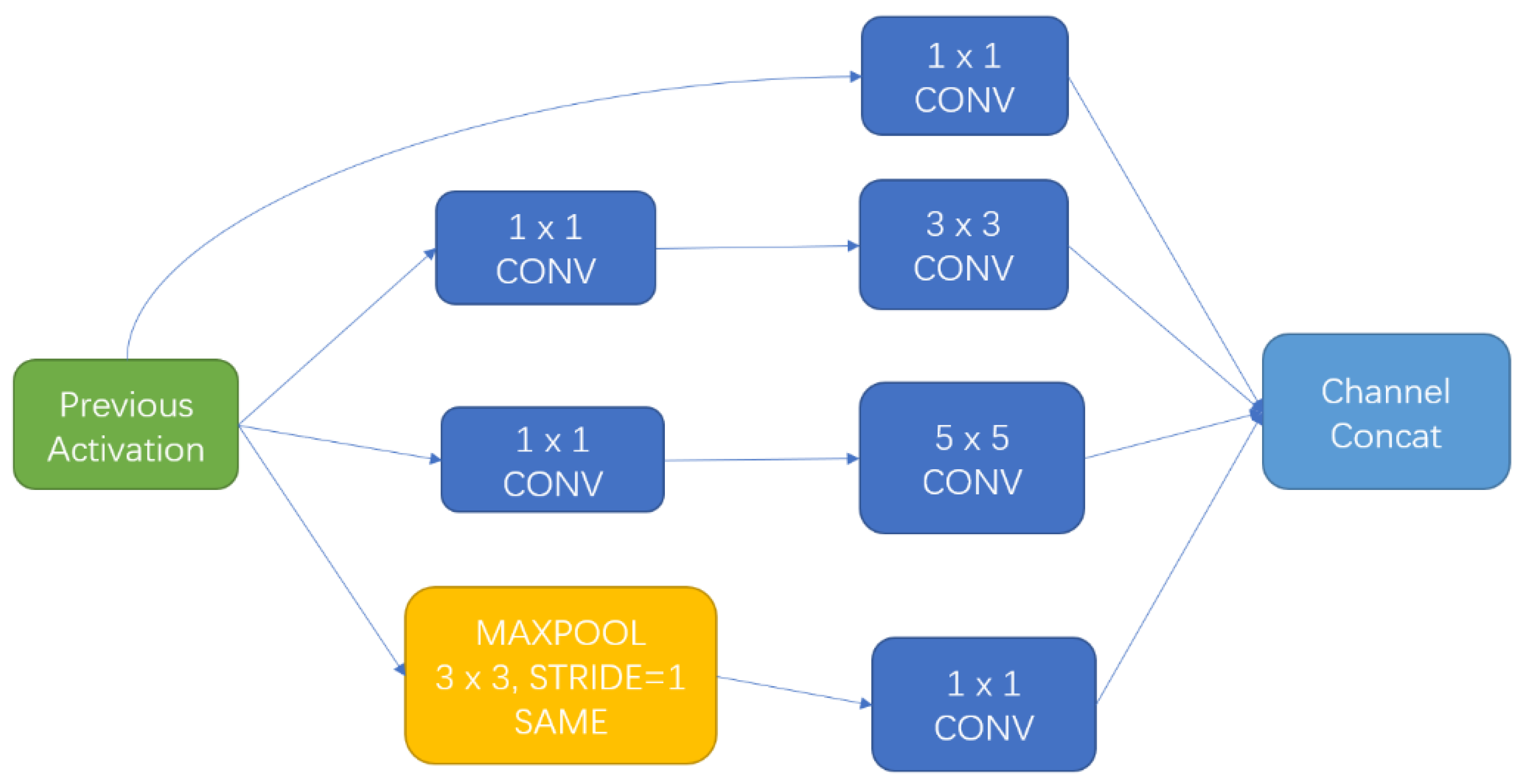
The concept of “Inception” was first proposed in the GoogLeNet structure [31]. Instead of stacking the network depth to improve the performance of the model, InceptionV3 achieves a better model performance by building a network that balances depth and width. The first few layers of the network consist of a common convolutional layer and a max pooling layer, followed by a stack of Inception modules with different structures. The structure of the Inception module is shown in Figure 4. The convolutions are of varied sizes of 1 × 1, 3 × 3, and 5 × 5. Additionally, it also contains a 3 × 3 pooling layer. These Inception modules help the model to save a lot of parameters, reduce overfitting, and increase the diversity of features.
2.3. Machine Learning
2.3.1. Random Forest
Random forest is a multifunctional machine-learning algorithm that was first proposed by Leo Breiman and Adele Cutler. It is a data dimensionality reduction tool used to handle missing values, outliers, and other important steps in data exploration with good results [32]. Many decision trees (weak classifiers) are generated in the random forest, and each tree gives its own classification choice. By combining multiple weak classifiers in a voting or averaging way, the overall model has a high accuracy and generalization performance. In this experiment, the number of decision trees was set to 100, and used Gini impurity to measure the quality of a split. Gini impurity is a common metric to measure classification performance. The smaller the Gini impurity, the higher the purity, the higher the degree of order of the set, and the better the classification.
2.3.2. Logistic Regression
Logistic regression does not solve the regression problem, but rather the classification problem. It is a typical linear classifier that learns sample characteristics to obtain hypothetical functions between labels by training the positive and negative examples in the data. Faced with a classification problem, a cost function is established, the optimization method is iterated to get the optimal model parameters, and then the model is validated. In this experiment, L2 regularization was used to penalize the loss function. It added a “penalty term” to the parameters after the loss function. This prevented the model from becoming complex with too many parameters, and thus reduced the overfitting of the model.
2.3.3. Support Vector Machine
In 1995, Cortes and Vapnik proposed the support vector machine approach [33]. This method can find the best compromise between the complexity of a model and the learning ability to obtain the best generalization capability based on the limited sample information. The core idea of SVM is to map the input space to a higher dimension by using kernel functions. In this experiment, the radial basis function kernel was used as the mapping function for the hyperplane.
2.4. Out-of-Fold Prediction
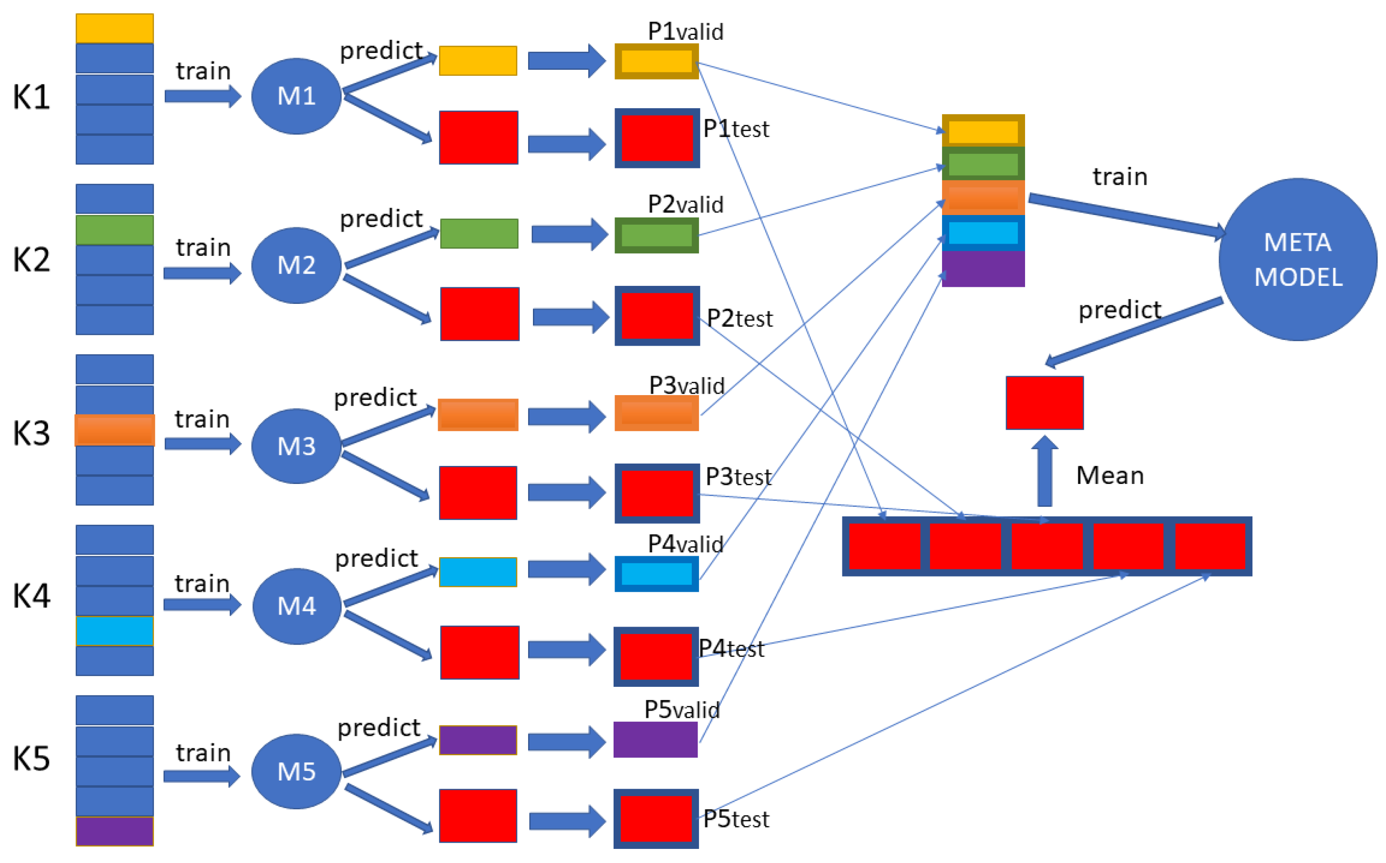
Machine-learning algorithms often use k-fold cross-validation to evaluate model performance. During k-fold cross-validation, the model makes predictions on test samples that are not used for training, and such predictions are called out-of-fold predictions. The process of out-of-fold prediction for this experiment is shown in Figure 5. The dataset was first divided into a training set and a test set at a ratio of 4:1. Next, the training set was divided equally into K groups, and each subset of data was made a validation set once. The rest of the K − 1 group subset of data was used as the training set. These training sets were then trained on the base-model so that K models were obtained; these are referred to as M1, M2...MK, and the datasets used to train these K models were called K1, K2...KK. After that, the trained M models were used to predict the test set and its corresponding validation set, and the prediction probabilities Ptest and Pvalid were saved for each class. so that after K models were predicted, there were a total of K different Pvalid and Ptest. These different Pvalid were stacked together as the feature input to the meta-model. At this point, the number of samples was exactly equal to the number of training sets. For different Ptest, the predicted probabilities corresponding to each class were summed and averaged, and the result was used as the test set of the meta-model. In this experiment, K was set to 5. Random forest, logistic regression, and support vector machine were used as the meta-model; and AlexNet, VGG16, ResNet50, DensenNet121, and InceptionV3 were used as the base-model.
2.5. Software and Hardware
The test software environment was a Windows 10 system using a PyTorch deep-learning open-source framework, and the programming language was Python. The computer had 32 GB of memory and was equipped with an Intel (R) Core (TM) i7-8700 CPU @ 3.20 GHz 3.19 GHz, and used an NVIDIA GeForce RTX 2080 (Nvidia Corporation, Santa Clara, CA, USA) to accelerate training. In this experiment, the AlexNet, VGG16, DenseNet121, ResNet50, and InceptionV3 models were all loaded with weights of more than 1000 classes, including 1.2 million images trained from ImageNet, and the softmax layer of the last layer of the model was changed from 1000 neurons to 5 neurons. The image input size for the InceptionV3 model was 299 × 299, while the input size of the other four models was 224 × 224. The learning rate was uniformly set as 1 × 10⁻⁴, the batch size was set as 16, the optimization function adopted SGD, and the momentum was set as 0.9 to accelerate the training. Before images were input to the model, the PyTorch script used three image-augmentation methods together on them. These three methods were image flipping, rotation, and scaling.
3. Results
3.1. Deep-Learning Model and Traditional Machine-Learning Model Accuracy
The expression of the accuracy rate (Acc) of this experiment’s calculation model was calculated as in Equation (1):
where nn is the total number of sample classes, i is the class label, nii is the number of samples predicted as class I, and ni is the total number of samples in class I.
In Table 2, we can see that among the five CNN models, the accuracy of DenseNet121 in the test set was 95.98%, which was higher than other models. The accuracies of InceptionV3, ResNet50, AlexNet, and VGG16 in the test set were 95.07%, 95.25%, 91.79%, and 93.35%, respectively. In the traditional machine-learning method, SVM achieved an accuracy of 73.20%, which is 11.77% higher than the lowest LR of 61.43%. Compared with the convolutional neural network, the traditional machine-learning methods were much less effective in identification. Convolutional neural networks can automatically extract useful features of images through convolutional layers, and then summarize and classify these features nicely through the final fully connected layer.
3.2. Accuracy and Confusion Matrix of the Model after Stacking Ensemble
The confusion matrix was used to compare the performance of the classifier. Each row of the confusion matrix represents examples of unpredicted peanut-leaf disease, and each column represents actual peanut-leaf disease. Based on the confusion matrix, three indicators—recall, precision, and weighted average score (F1 score) of recall accuracy—were used to evaluate the performance of the model. In this experiment, F1(i) was used to evaluate the performance of model corresponding to each class, and F1 used the F1(i) of each class to weigh the performance of the whole model. Equations (2)–(5) given the calculation of these indicators.
where precision(i) is the precision corresponding to class I, TP is the number of correct answers to the prediction, and FP is the number of other classes predicted as this class by error.
where recall(i) is the recall rate corresponding to class I, and FN is the number of classes that are predicted to be other classes.
where F1(i) is the weighted average score of the recall accuracy corresponding to each class.
where F1 is the weighting of the recall accuracy of the entire model’s average score.
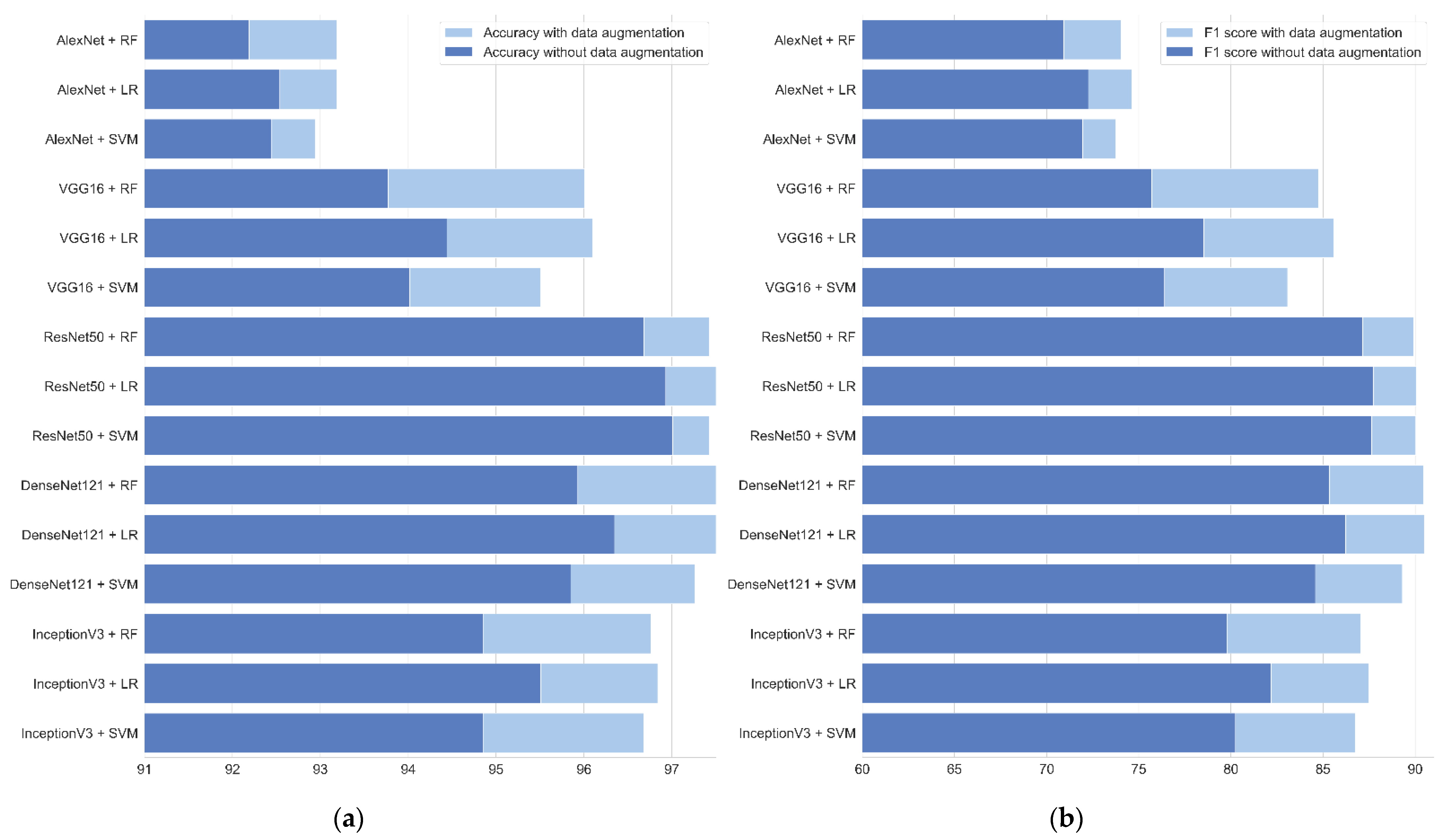
As shown in Figure 6, Table 3 and Table 4, the accuracy and F1 score of each model were improved after using the stacking ensemble. In this experiment, the highest accuracy of the models reached 97.59%, and there were two ways to achieve this accuracy. One was to use ResNet50 as the base-model for extracting the features of the images, and then use LR to ensemble the five M models. Compared with the accuracy before the ensemble, the accuracy of the models improved by 2.37%. Another way to achieve the same accuracy was to use DenseNet121 to extract image features and then ensemble the model with RF. As shown in Table 2, without the use of out-of-fold predictions, the deep-learning methods were all very effective in the identification of peanut-leaf diseases. Each of the five base-models used in this experiment achieved an accuracy of more than 90% for the dataset. In the image-classification problem, a higher classification accuracy meant that it was harder to improve the accuracy any further. However, after using out-of-fold prediction, the accuracy of the five models was improved. Even when the accuracy was already high without using out-of-fold prediction, the accuracy was still improved by 1–3%. By training the meta-model using out-of-fold predictions from the base-model, the meta-model could view and exploit the expected behavior of each base-model when run on unseen data, as was the case in practice when using ensembles to make predictions on new data. The main point is that when the predictions of base-model were used as the input features of the meta-model, the meta-model was able to distinguish between models that performed well in the base-model and the models that performed poorly. It is also important to note that a feature input into the meta-model did not depend on its corresponding target in the base-model. This is because these features were generated using information that excluded the corresponding target from the base-model fitting process.
3.3. Effect of Data Augmentation on Model Accuracy and F1 Score
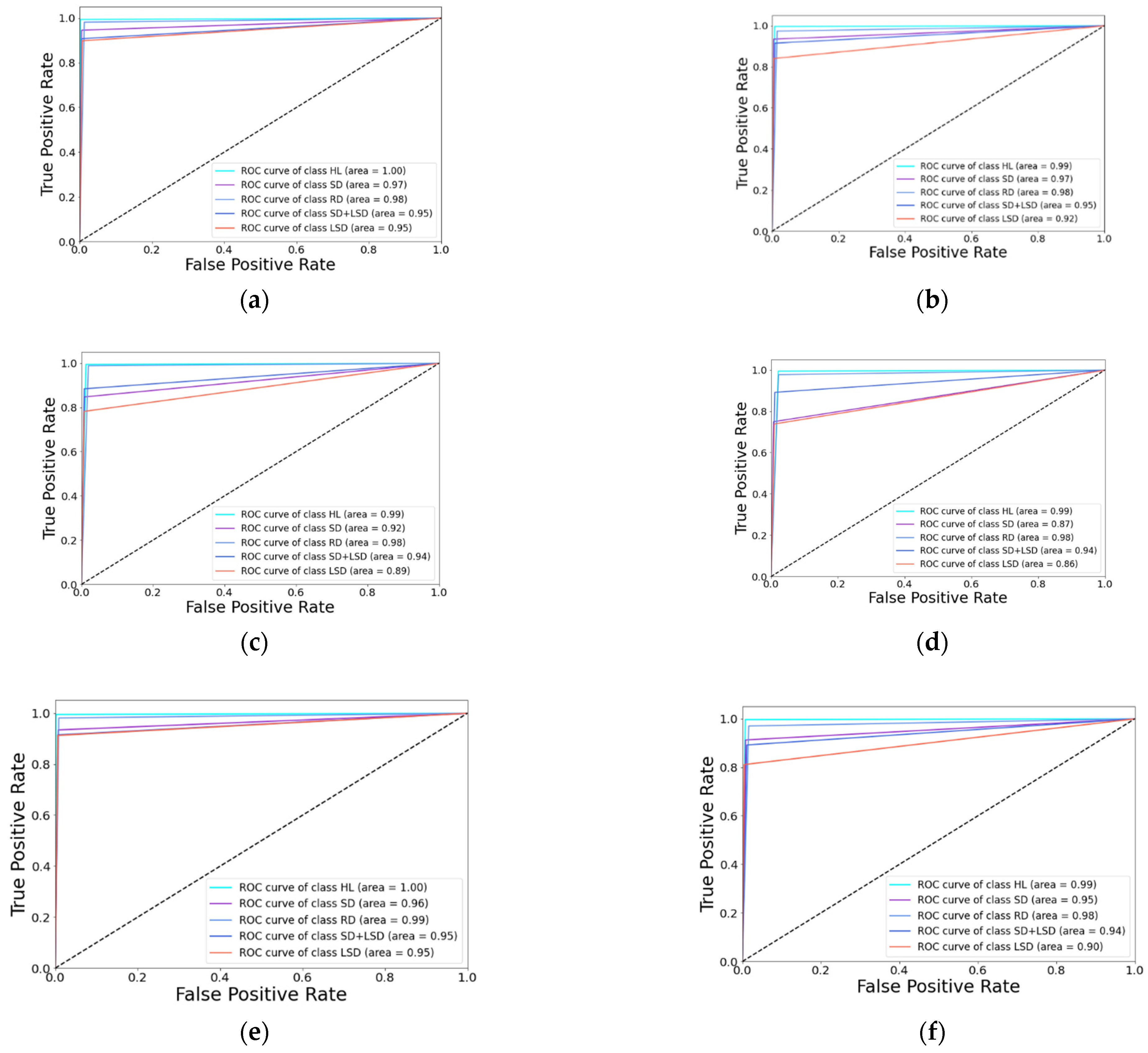
The area under the receiver operating characteristic (AUC–ROC) curve and AUC curves are often used to evaluate the performance of a machine-learning algorithm as well. The ROC curve plots the difference between the false positive rate (FPR) and true positive rate (TPR). A larger area under the curve means that the classifier has a better classification performance for that class. The formula is defined as in Equations (6) and (7):
where TPR is the amount of positive data that is correctly predicted as positive with respect to all positive data.
where TN represents a class that is truly false and predicted to be false, and FPR represents the amount of negative data points that are wrongly predicted as positive with respect to all negative data.
It is necessary to emphasize the data used during training. For example, as shown in Table 3, Table 4, Figure 6, and Figure 7, when using the data-augmentation technique in this experiment, the accuracy of each model was improved, as well as the F1 score, which is an important measure of the performance of a machine-learning model that weighs the recall and precision of the model to give an overall assessment of the performance of the model. Without data augmentation, the maximum overall F1 score of VGG16 after ensemble was 78.52. After training with data augmentation, the maximum F1 score reached 85.60. A larger F1 score meant that the classifier was more stable and did not easily misclassify this class into other classes. Figure 7 randomly selects three of the 30 models and presents their ROC curves. According to Figure 7, the curve coverage area of the SD and LSD classes improved after using the data-augmentation method, which indicates that the classification performance of the classifier for the SD and LSD classes was improved. Many neural networks have millions of parameters, and making these parameters work correctly requires large amounts of data on which to train. Data-augmentation techniques can improve the generalizability of a model by providing more training samples for the network and reducing the model’s dependence on certain attributes.
3.4. Identify Performance of Each Class after Model Ensemble
After feature extraction from the base-model, the ensemble of features with a different meta-model gave different results. As shown in Table 3 and Table 4, the F1 score of all five base-models were maximally improved after ensemble with LR, and all deep-learning models except DenseNet121 achieved the highest accuracy. The ensemble of features using the meta-model improved the accuracy of the models compared to the nonstacking models. As can be seen in Table 5, the best ensemble of all models had a very high identification accuracy for HD. For SD and LSD identification, the deeper models like DensenNet121 and ResNet50 had significantly higher maximum F1 scores after ensemble than AlexNet and VGG16. Likewise, after LR ensemble, ResNet50 achieved the highest recall and precision in RD and RD + SD. ResNet50 and DenseNet121 benefited from the shortcut structure, which progressed to full use of the information in each feature map, deepening the network layers while reducing the impact of the gradient explosion on training.
4. Discussion
Machine-learning models have been developed constantly and have become very effective in the classification of images. They provide a feasible method for the identification of most plant-leaf diseases. However, the effectiveness of machine learning on the identification of peanut-leaf diseases have not been previously reported. Accurate diagnosis of peanut-leaf disease classes, and timely treatment of the disease are practical guidance for peanut production.
In this study, traditional machine-learning methods and deep-learning models were used for the identification of peanut-leaf diseases. After that, the traditional machine-learning methods and deep-learning models were combined by stacking ensemble. The training strategies of data augmentation and transfer learning were also used to evaluate the fitting performance of the models on the dataset of peanut-leaf diseases. The results showed that the deep-learning models had more robustness than the traditional machine-learning methods when identifying peanut-leaf diseases. The models with deeper network layers such as Densenet121 and Resnet50 performed better than shallow and wide networks when used as the base-model. The performance of logistic regression classification was worse than support vector machine and random forest classification, but logistic regression as the meta-model could best improve the accuracy and F1 score of the base-model.
In the literature, different traditional machine-learning methods of classification, such as clustering [10], stacking [12], and low-dimensional to high-dimensional mapping [11], have been shown to be applicable to the classification of a wide range of plant leaves. However, to obtain high accuracy and robustness, it is necessary to artificially extract features, and the quality of the extracted features directly affects the performance of the model.
Deep-learning models have excellent performance in classifying images due to the rotation invariance, translation invariance, and sparse parameters of the convolutional layer [27]. Mohanty verified that deep-learning models can be applied to disease identification in a variety of plant leaves [25]. In order to improve the accuracy of recognition, various deep-learning training strategies have also been successfully applied to plant image classification, such as data augmentation [23], transfer learning [21], and semisupervised learning [24]. The five selected deep-learning models in our study still had a good classification performance in the dataset collected in the field environment. The results showed that the deep-learning models were still able to accurately identify peanut-leaf diseases in complex picture backgrounds. The deep-learning model with deeper network layers fit better to the peanut-leaf-disease dataset used in this study. Moreover, when the deep-learning model was used as a meta-model, the better the classification performance it had, the better the performance it achieved after the stacking ensemble.
5. Conclusions
Peanut-leaf disease is an important reason for the decline of peanut yields and quality. If a disease of peanut leaves can be detected in time, preventive measures can be taken as soon as possible to reduce the loss of crops.
To solve the problem of peanut-leaf diseases, this paper combined deep-learning models and traditional machine-learning methods to identify four peanut-leaf diseases. The networks with deeper layers, like ResNet50 and DenseNet121, had the best prediction performance for datasets. In the case of data augmentation, the highest accuracy reached 97.59%, and the F1 score reached 90.50 using the traditional machine-learning method for the ensemble.
In this paper, a leaf showing two diseases, a mixture of rust and scorch diseases, was identified for the first time. The best identification performance was achieved by ResNet50 combined with the LR model, which had a recall rate of 93.08, and the corresponding F1 score of 93.80 was the highest among all models. The other models also achieved good identification performance, indicating that the machine-learning method is still a powerful tool for identifying peanut-leaf diseases, including in the case of a peanut leaf showing two diseases at the same time.
At present, although the laboratory model of the highest recognition rate reached 97.59%, the field environment is complicated, and recognition of peanut-leaf diseases will still encounter many problems, such as a peanut leaf appearing at the same time as a number of different leaves, the degree of disease occurring, and the difficulty of training data collection. Further studies are needed to improve these problems.
Author Contributions
Conceptualization, H.Q.; methodology, H.Q.; software, Y.L.; validation, J.Z.; formal analysis, Y.L., Q.D.; investigation, Y.L.; resources, Y.L.; data curation, Y.L.; writing—original draft preparation, Y.L.; writing—review and editing, H.Q., Q.D.; visualization, J.Z.; supervision, H.Q. All authors have read and agreed to the published version of the manuscript.
Funding
This research was funded by the Key-Area Research and Development Program of Guangdong Province (2019B020214003), and characteristic innovation projects of the Guangdong Provincial Department of Education in 2019 (2019KTSCX015).
Institutional Review Board Statement
Not applicable.
Informed Consent Statement
Not applicable.
Data Availability Statement
Not applicable.
Conflicts of Interest
The authors declare no conflict of interest.
References
- Li, S.; Hong, Y.; Chen, X.; Liang, X. Present Situation and Development Strategies of Peanut Production, Breeding and Seed Industry in Guangdong. Guangdong Agric. Sci. 2020, 47, 78–83. [Google Scholar]
- Singh, M.P.; Erickson, J.E.; Boote, K.J.; Tillman, B.L.; Jones, J.W.; Van Bruggen, A.H. Late Leaf Spot Effects on Growth, Photosynthesis, and Yield in Peanut Cultivars of Differing Resistance. Agron. J. 2011, 103, 85–91. [Google Scholar] [CrossRef] [Green Version]
- Qi, H.; Zhu, B.; Kong, L.; Yang, W.; Zou, J.; Lan, Y.; Zhang, L. Hyperspectral inversion model of chlorophyll content in peanut leaves. Appl. Sci. 2020, 10, 2259. [Google Scholar] [CrossRef] [Green Version]
- Beltran-Perez, C.; Wei, H.-L.; Rubio-Solis, A. Generalized Multiscale RBF Networks and the DCT for Breast Cancer Detection. Int. J. Autom. Comput. 2020, 17, 55–70. [Google Scholar] [CrossRef]
- Pham, B.T.; Jaafari, A.; Avand, M.; Al-Ansari, N.; Dinh Du, T.; Yen, H.P.H.; Phong, T.V.; Nguyen, D.H.; Le, H.V.; Mafi-Gholami, D.; et al. Performance evaluation of machine learning methods for forest fire modeling and prediction. Symmetry 2020, 12, 1022. [Google Scholar] [CrossRef]
- Kranjčić, N.; Medak, D.; Župan, R.; Rezo, M. Machine learning methods for classification of the green infrastructure in city areas. ISPRS Int. J. Geo Inf. 2019, 8, 463. [Google Scholar] [CrossRef] [Green Version]
- Bandi, S.R.; Varadharajan, A.; Chinnasamy, A. Technology, Performance evaluation of various statistical classifiers in detecting the diseased citrus leaves. Int. J. Eng. Sci. Technol. 2013, 5, 298–307. [Google Scholar]
- Wang, G.; Sun, Y.; Wang, J. Automatic Image-Based Plant Disease Severity Estimation Using Deep Learning. Comput. Intell. Neurosci. 2017, 2017, 2917536. [Google Scholar] [CrossRef] [PubMed] [Green Version]
- Zheng, Y.; Zhong, G.; Wang, Q.; Zhao, Y. Method of Leaf Identification Based on Multi-feature Dimension Reduction. Nongye Jixie Xuebao Trans. Chin. Soc. Agric. Mach. 2017, 48, 30–37. [Google Scholar]
- Wang, S.; He, D.; Li, W.; Wang, Y. Plant leaf disease recognition based on kernel K-means clustering algorithm. Nongye Jixie Xuebao Trans. Chin. Soc. Agric. Mach. 2009, 40, 152–155. [Google Scholar]
- Es-saady, Y.; El Massi, I.; El Yassa, M.; Mammass, D.; Benazoun, A. Automatic recognition of plant leaves diseases based on serial combination of two SVM classifiers. In Proceedings of the 2016 International Conference on Electrical and Information Technologies (ICEIT), Tangiers, Morocco, 4–7 May 2016; pp. 561–566. [Google Scholar]
- Azadbakht, M.; Ashourloo, D.; Aghighi, H.; Radiom, S.; Alimohammadi, A.J.C.; Agriculture, E. Wheat leaf rust detection at canopy scale under different LAI levels using machine learning techniques. Comput. Electron. Agric. 2018, 156, 119–128. [Google Scholar] [CrossRef]
- Feng, T.; Xiaodan, M. The method of recognition of damage by disease and insect based on laminae. J. Agric. Mech. Res. 2009, 6, 41–43. [Google Scholar]
- Wang, H.; Li, G.; Ma, Z.; Li, X. Image recognition of plant diseases based on principal component analysis and neural networks. In Proceedings of the 2012 8th International Conference on Natural Computation, Chongqing, China, 29–31 May 2012; pp. 246–251. [Google Scholar]
- Huang, J.; Kingsbury, B. Audio-visual deep learning for noise robust speech recognition. In Proceedings of the 2013 IEEE International Conference on Acoustics, Speech and Signal Processing, Vancouver, BC, Canada, 26–31 May 2013; pp. 7596–7599. [Google Scholar]
- Yu, D.; Deng, L. Automatic Speech Recognition; Springer: Berlin/Heidelberg, Germany, 2016. [Google Scholar]
- Tao, J.; Wang, H.; Zhang, X.; Li, X.; Yang, H. An object detection system based on YOLO in traffic scene. In Proceedings of the 2017 6th International Conference on Computer Science and Network Technology (ICCSNT), Chongqing, China, 29–31 May 2017; pp. 315–319. [Google Scholar]
- Zhu, Y.; Fan, H.; Yuan, K. Facial expression recognition research based on deep learning. arXiv 2019, arXiv:1904.09737. [Google Scholar]
- Cao, Z.; Simon, T.; Wei, S.-E.; Sheikh, Y. Realtime multi-person 2d pose estimation using part affinity fields. In Proceedings of the IEEE Conference on Computer Vision and Pattern Recognition, Honolulu, HI, USA, 21–26 July 2017; pp. 7291–7299. [Google Scholar]
- Toshev, A.; Szegedy, C. Deeppose: Human pose estimation via deep neural networks. In Proceedings of the IEEE Conference on Computer Vision and Pattern Recognition, Columbus, OH, USA, 23–28 June 2014; pp. 1653–1660. [Google Scholar]
- Geetharamani, G.; Pandian, A. Identification of plant leaf diseases using a nine-layer deep convolutional neural network. Comput. Electr. Eng. 2019, 76, 323–338. [Google Scholar]
- Hang, J.; Zhang, D.; Chen, P.; Zhang, J.; Wang, B. Classification of Plant Leaf Diseases Based on Improved Convolutional Neural Network. Sensors 2019, 19, 4161. [Google Scholar] [CrossRef] [Green Version]
- Zhang, S.; Zhang, S.; Zhang, C.; Wang, X.; Shi, Y. Cucumber leaf disease identification with global pooling dilated convolutional neural network. Comput. Electron. Agric. 2019, 162, 422–430. [Google Scholar] [CrossRef]
- Amorim, W.P.; Tetila, E.C.; Pistori, H.; Papa, J.P. Semi-Supervised Learning with Convolutional Neural Networks for UAV images Automatic Recognition. Comput. Electron. Agric. 2019, 164, 104932. [Google Scholar] [CrossRef]
- Mohanty, S.P.; Hughes, D.P.; Salathé, M. Using deep learning for image-based plant disease detection. Front. Plant Sci. 2016, 7, 1419. [Google Scholar] [CrossRef] [PubMed] [Green Version]
- LeCun, Y.; Bottou, L.; Bengio, Y.; Haffner, P. Gradient-based learning applied to document recognition. Proc. IEEE 1998, 86, 2278–2324. [Google Scholar] [CrossRef] [Green Version]
- Krizhevsky, A.; Sutskever, I.; Hinton, G.E. Imagenet classification with deep convolutional neural networks. Adv. Neural Inf. Process. Syst. 2012, 25, 1097–1105. [Google Scholar] [CrossRef]
- Simonyan, K.; Zisserman, A. Very deep convolutional networks for large-scale image recognition. arXiv 2014, arXiv:1409.1556. [Google Scholar]
- He, K.; Zhang, X.; Ren, S.; Sun, J. Deep residual learning for image recognition. In Proceedings of the IEEE Conference on Computer Vision and Pattern Recognition, Las Vegas, NV, USA, 27–30 June 2016; pp. 770–778. [Google Scholar]
- Huang, G.; Liu, Z.; Van Der Maaten, L.; Weinberger, K.Q. Densely connected convolutional networks. In Proceedings of the IEEE Conference on Computer Vision and Pattern Recognition, Honolulu, HI, USA, 21–26 July 2017; pp. 4700–4708. [Google Scholar]
- Szegedy, C.; Vanhoucke, V.; Ioffe, S.; Shlens, J.; Wojna, Z. Rethinking the inception architecture for computer vision. In Proceedings of the IEEE Conference on Computer Vision and Pattern Recognition, Las Vegas, NV, USA, 27–30 June 2016; pp. 2818–2826. [Google Scholar]
- Breiman, L. Random forests. Mach. Learn. 2001, 45, 5–32. [Google Scholar] [CrossRef] [Green Version]
- Cortes, C.; Vapnik, V. Support-Vector Networks. Mach. Learn. 1995, 20, 273–297. [Google Scholar] [CrossRef]
Figure 1.
The original images of peanut leaves collected by mobile phone.

Figure 2.
Condition of leaves, from left to right: healthy, simultaneously suffering from rust and scorch disease, rust disease, leaf-spot disease, and scorch disease.
Figure 2.
Condition of leaves, from left to right: healthy, simultaneously suffering from rust and scorch disease, rust disease, leaf-spot disease, and scorch disease.

Figure 3.
A typical convolutional neural network structure.

Figure 4.
Inception module structure.

Figure 5.
Out-of-fold prediction process.

Figure 6.
(a) Accuracy of model ensemble; (b) F1 score of model ensemble.

Figure 7.
ROC curves for the model after ensemble. (a) ROC curve DenseNet121 + LR data augmentation; (b) ROC curve DenseNet121 + LR without data augmentation; (c) ROC curve VGG16 + SVM data augmentation; (d) ROC curve VGG16 + SVM without data augmentation; (e) ROC curve DenseNet121 + RF data augmentation; (f) ROC curve DenseNet121 + RF without data augmentation.


Table 1.
Information for the division of datasets.
| Train_Set | Test_Set | |
|---|---|---|
| Healthy leaves (HL) | 2564 | 641 |
| Scorch disease (SD) | 371 | 92 |
| Rust disease (RD) | 1087 | 272 |
| Leaf-spot disease (LSD) | 277 | 69 |
| Both scorch and rust disease (SD + RD) | 526 | 130 |
| Total: 6029 | ||
Table 2.
Prediction accuracy of M models in deep learning and traditional machine learning.
| Model | Data Augmentation | Without Data Augmentation | ||||||||||
|---|---|---|---|---|---|---|---|---|---|---|---|---|
| M1 | M2 | M3 | M4 | M5 | Mean | M1 | M2 | M3 | M4 | M5 | Mean | |
| AlexNet | 91.61 | 91.40 | 92.02 | 92.33 | 91.61 | 91.79 | 90.36 | 89.95 | 92.33 | 90.78 | 91.50 | 90.38 |
| VGG16 | 93.78 | 93.89 | 95.34 | 92.54 | 91.19 | 93.35 | 92.64 | 93.26 | 92.64 | 94.09 | 93.06 | 93.14 |
| ResNet50 | 96.58 | 94.92 | 94.61 | 94.92 | 95.23 | 95.25 | 94.40 | 93.78 | 94.20 | 94.30 | 95.13 | 94.36 |
| DenseNet121 | 96.68 | 96.68 | 95.85 | 95.85 | 94.82 | 95.98 | 92.64 | 95.44 | 93.37 | 93.58 | 95.03 | 94.01 |
| InceptionV3 | 95.03 | 95.75 | 94.51 | 93.68 | 96.37 | 95.07 | 91.92 | 91.92 | 91.71 | 90.26 | 93.68 | 91.90 |
| SVM | 73.56 | 73.44 | 72.98 | 72.55 | 73.48 | 73.20 | 70.76 | 70.43 | 70.27 | 69.68 | 70.51 | 70.33 |
| RF | 72.33 | 71.98 | 72.05 | 72.16 | 71.95 | 72.09 | 69.52 | 69.35 | 69.93 | 70.18 | 69.35 | 69.67 |
| LR | 61.35 | 62.01 | 61.48 | 61.24 | 61.08 | 61.43 | 59.47 | 59.47 | 59.80 | 60.05 | 59.22 | 59.60 |
Table 3.
Accuracy of the model ensemble with and without data augmentation.
| Model | Accuracy | |||||||
|---|---|---|---|---|---|---|---|---|
| Data Augmentation | Without Data Augmentation | |||||||
| RF | LR | SVM | WE 1 | RF | LR | SVM | WE | |
| AlexNet | 93.19 | 93.19 | 92.94 | 91.79 | 92.19 | 92.54 | 92.44 | 90.98 |
| VGG16 | 96.01 | 96.10 | 95.51 | 93.35 | 93.77 | 94.44 | 94.02 | 93.14 |
| ResNet50 | 97.43 | 97.59 | 97.43 | 95.25 | 96.68 | 96.93 | 97.01 | 94.36 |
| DenseNet121 | 97.59 | 97.51 | 97.26 | 95.98 | 95.93 | 96.35 | 95.85 | 94.01 |
| InceptionV3 | 96.76 | 96.84 | 96.68 | 95.07 | 94.85 | 95.51 | 94.85 | 93.37 |
1 Without ensemble.
Table 4.
F1 scores for the model ensemble with and without data augmentation.
| Model | F1 Score | |||||
|---|---|---|---|---|---|---|
| Data Augmentation | Without Data Augmentation | |||||
| RF | LR | SVM | RF | LR | SVM | |
| AlexNet | 74.04 | 74.63 | 73.77 | 73.77 | 72.27 | 71.96 |
| VGG16 | 84.75 | 85.60 | 83.08 | 83.08 | 78.52 | 76.40 |
| ResNet50 | 89.93 | 90.07 | 90.04 | 90.04 | 87.74 | 87.64 |
| DenseNet121 | 90.45 | 90.50 | 89.31 | 89.31 | 86.22 | 84.59 |
| InceptionV3 | 80.25 | 87.48 | 86.75 | 79.78 | 82.17 | 86.75 |
Table 5.
Recall and precision of the best ensemble for each class.
| AlexNet | VGG16 | ResNet50 | DenseNet121 | InceptionV3 | |||||||||||
|---|---|---|---|---|---|---|---|---|---|---|---|---|---|---|---|
| Recall | Precision | Meta 1 | Recall | Precision | Meta | Recall | Precision | Meta | Recall | Precision | Meta | Recall | Precision | Meta | |
| HD | 99.38 | 97.25 | RF | 99.53 | 98.76 | LR | 99.69 | 99.84 | LR | 99.53 | 99.84 | LR | 100.00 | 99.53 | LR |
| SD | 75.00 | 88.46 | RF | 85.87 | 92.94 | LR | 93.48 | 95.56 | SVM | 95.65 | 93.62 | SVM | 92.39 | 94.44 | LR |
| RD | 97.06 | 90.10 | LR | 96.32 | 95.62 | RF | 98.53 | 96.75 | LR | 98.53 | 96.75 | RF | 97.79 | 94.66 | RF |
| SD + RD | 81.54 | 92.98 | LR | 92.31 | 90.91 | RF | 93.08 | 94.53 | LR | 90.77 | 95.93 | LR | 90.00 | 94.35 | SVM |
| LSD | 71.01 | 75.38 | LR | 84.06 | 87.88 | RF | 91.30 | 90.00 | RF | 89.86 | 92.54 | RF | 85.51 | 88.06 | RF |
1 Meta-model.
Publisher’s Note: MDPI stays neutral with regard to jurisdictional claims in published maps and institutional affiliations. |
© 2021 by the authors. Licensee MDPI, Basel, Switzerland. This article is an open access article distributed under the terms and conditions of the Creative Commons Attribution (CC BY) license (http://creativecommons.org/licenses/by/4.0/).
Share and Cite
MDPI and ACS Style
Qi, H.; Liang, Y.; Ding, Q.; Zou, J. Automatic Identification of Peanut-Leaf Diseases Based on Stack Ensemble. Appl. Sci. 2021, 11, 1950. https://0-doi-org.brum.beds.ac.uk/10.3390/app11041950
AMA Style
Qi H, Liang Y, Ding Q, Zou J. Automatic Identification of Peanut-Leaf Diseases Based on Stack Ensemble. Applied Sciences. 2021; 11(4):1950. https://0-doi-org.brum.beds.ac.uk/10.3390/app11041950
Chicago/Turabian StyleQi, Haixia, Yu Liang, Quanchen Ding, and Jun Zou. 2021. "Automatic Identification of Peanut-Leaf Diseases Based on Stack Ensemble" Applied Sciences 11, no. 4: 1950. https://0-doi-org.brum.beds.ac.uk/10.3390/app11041950
Note that from the first issue of 2016, this journal uses article numbers instead of page numbers. See further details here.