Statistical Analysis of Nanofiber Mat AFM Images by Gray-Scale-Resolved Hurst Exponent Distributions

Abstract

Two-dimensional structures, either periodic or random, can be classified by diverse mathematical methods. Quantitative descriptions of such surfaces, however, are scarce since bijective definitions must be found to measure unique dependency between described structures and the chosen quantitative parameters. To solve this problem, we use statistical analysis of periodic fibrous structures by Hurst exponent distributions. Although such a Hurst exponent approach was suggested some years ago, the quantitative analysis of atomic force microscopy (AFM) images of nanofiber mats in such a way was described only recently. In this paper, we discuss the influence of typical AFM image post-processing steps on the gray-scale-resolved Hurst exponent distribution. Examples of these steps are polynomial background subtraction, aligning rows, deleting horizontal errors and sharpening. Our results show that while characteristic features of these false-color images may be shifted in terms of gray-channel and Hurst exponent, they can still be used to identify AFM images and, in the next step, to quantitatively describe AFM images of nanofibrous surfaces. Such a gray-channel approach can be regarded as a simple way to include some information about the 3D structure of the image.

1. Introduction

Electrospinning finds nowadays more and more frequent application in preparing nanofibers with diameters in the range of few ten to some hundred nanometers. Such applications concern diverse polymers, polymer blends or polymers with embedded nanoparticles [1,2,3,4,5]. Such nanofiber mats can be used in a broad range of possible applications, from filters [6,7] and catalyzers [8,9] to tissue engineering and cell growth [10,11,12,13].

For many of these applications, it is necessary to measure the fiber diameter distribution or the fiber orientation [14,15,16]. Other parameters, such as the pore size distribution, are also often important, but less easy to measure [17,18].

Generally, highly resolved images of such nanofiber mats, taken by scanning electron microscopy (SEM) or other techniques, allow for comparing optically different nanofiber mats. Such a procedure can be used for a subjective description of these nanofiber mats. On the other hand, only few quantitative parameters exist which can be used for objective descriptions of such high-resolution images and correspondingly reliable quantitative comparison.

One of these mathematical parameters is the so-called fractal dimension which can be used to describe defects in regular fabrics and may be suitable to describe the fiber orientation distribution in a nanofiber mat, too [19,20,21]. More special methods are based on the calculation of the succolarity, which can be used to describe the percolation of an image [22], or the lacunarity, which detects spatial continuity of surfaces [23,24]. Another widely used approach uses the so-called Hurst exponent which can be derived from an image by applying a random walking on this image [25,26] and has been applied on microscopic images of different textile fabrics before [27,28,29,30]. Only recently, we have shown for the first time that such Hurst exponent calculations can be applied to differentiate between atomic force microscopy (AFM) images of different nanofiber mats [31]. Such AFM images, however, are usually post-treated to reduce typical errors, such as horizontal line errors, or noise as well as to sharpen them.

The Hurst exponent has many applications in analysis of fractality, self-similarities and auto-correlations of various types of data. As an example on image analysis, the Hurst exponent was used to estimate the fractal dimension of a 3D landscape and quantify the landscape diversity [32,33]. Our approach is analogous, but only to some extent, as the analyzed textiles are much flatter that a landscape.

This paper contains the first report on the influence of typical post-treatment steps on the calculation of gray-scale-resolved Hurst exponent distributions—an approach which performs multiple random walking experiments on several sub-images split—into different grayscales derived from the original. Our research demonstrates that while the distributions themselves are modified by such post-treatment steps, their characteristics remain and can thus be used to quantitatively describe AFM images of electrospun nanofiber mats. Such a gray scale approach can be used to collect information about the 3D structure of the image in a simpler manner than a landscape analysis.

2. Materials and Methods

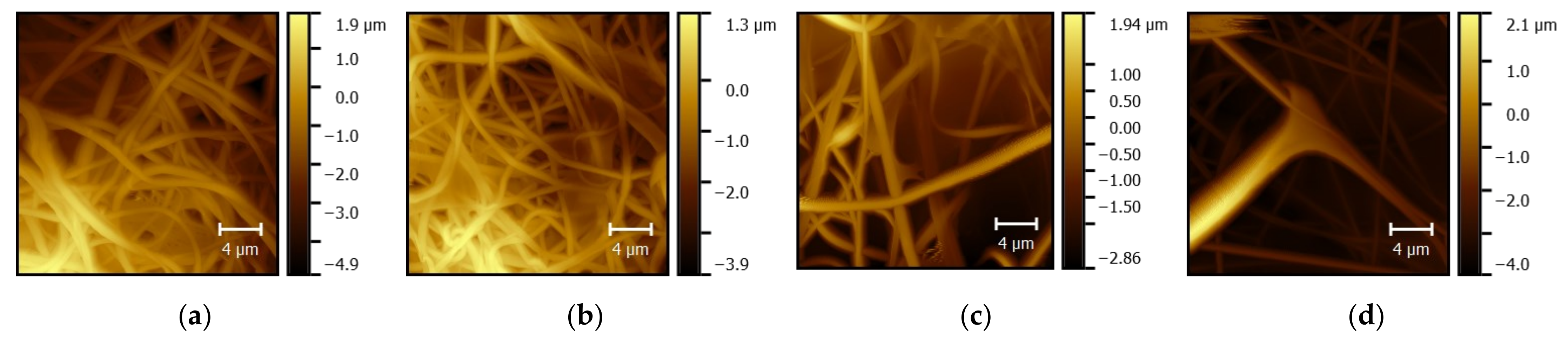
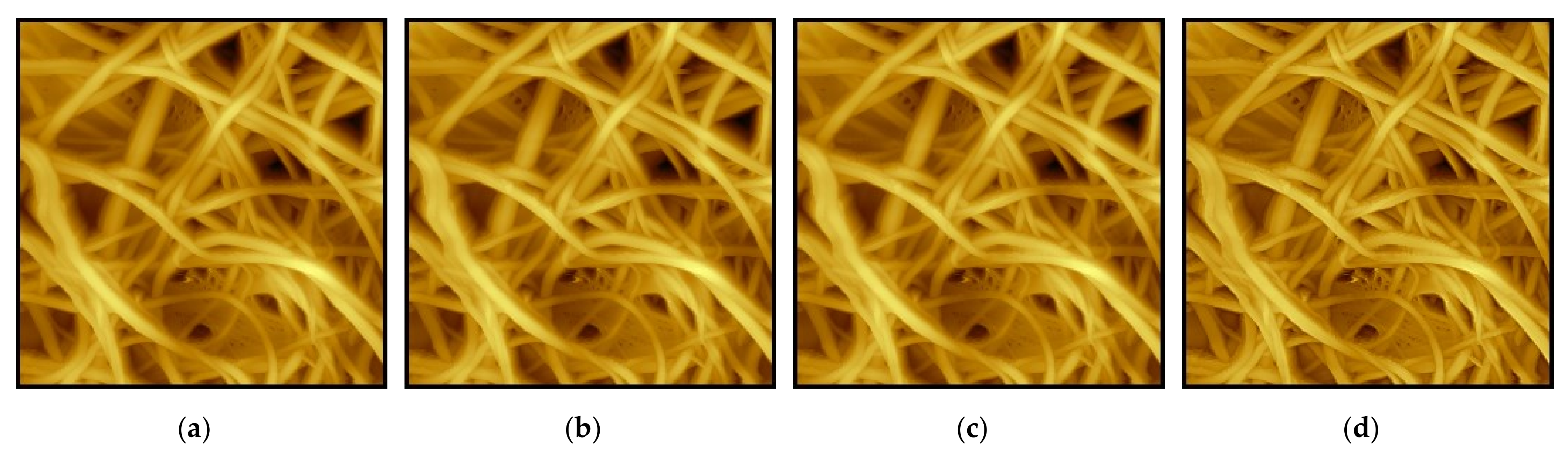
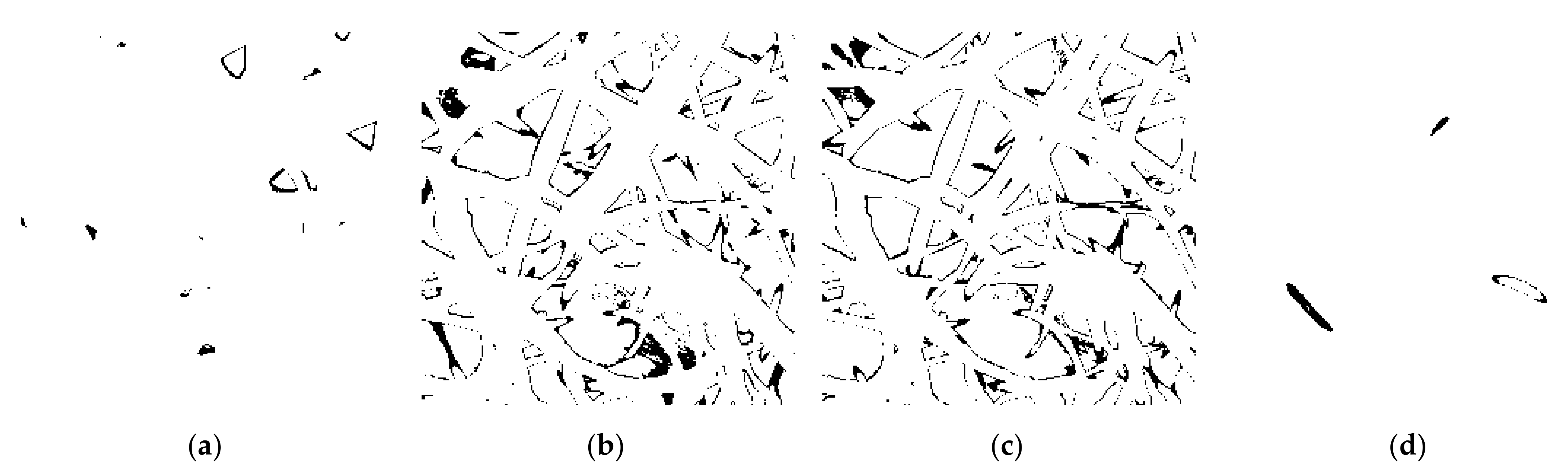
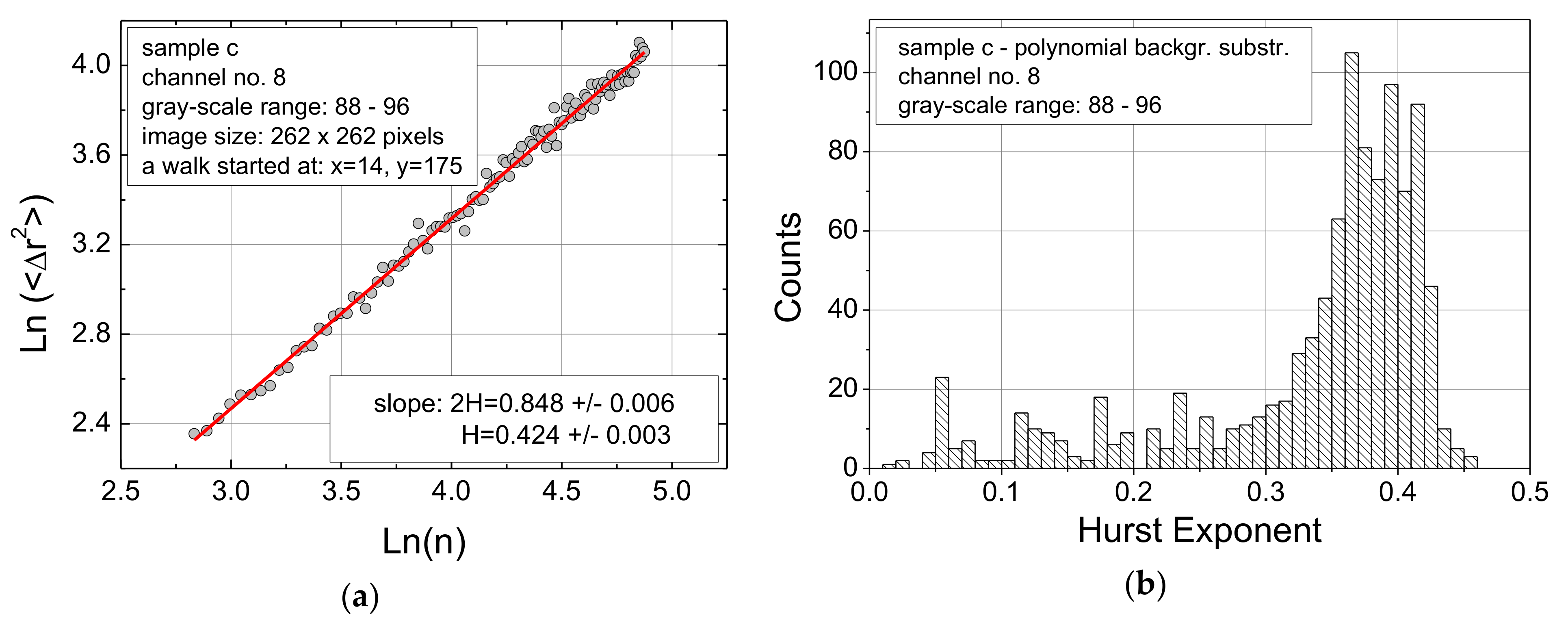
Samples for AFM investigations were prepared by electrospinning with a wire-based electrospinning machine Nanospider Lab (Elmarco Ltd., Liberec, Czech Republic), using the following spinning parameters: voltage 80 kV, nozzle diameter 0.9 mm, carriage speed 100 mm/s, distance between bottom electrode and substrate 240 mm, distance between ground electrode and substrate 50 mm, temperature in the spinning chamber 22 °C and a relative humidity of 32–33%.

To prepare the spinning solution, 16% polyacrylonitrile (PAN) (X-Pan, copolymer with 6% methyl methacrylate, from Dralon, Dormagen, Germany) were dissolved in dimethyl sulfoxide (DMSO, min 99.9%, S3 Chemicals, Bad Oeynhausen, Germany) by vigorously stirring at room temperature for 2 h.

The nanofiber mats were detached from the polypropylene substrate after electrospinning and glued on glass slides for AFM investigations.

The surfaces of the electrospun nanofiber mats were investigated by a FlexAFM (Nanosurf, Liestal, Switzerland) with an SHR300 cantilever (tip diameter 1 nm) in the dynamic mode. The sharp tip is supportive to avoid moving the nanofibers erroneously. Images sizes covered areas of 25 µm × 25 µm, the lateral resolution is ~100 nm. Approach parameters were optimized according to these surfaces (setpoint 60%, P-gain 750, I-gain 1200–1300 and D-gain 100, where the setpoint describes the oscillation amplitude of the cantilever, while P, I and D describe the proportional, integral and differential part of a common PID controller, respectively).

Post-processing was performed in Gwyddion 2.51 software, using the following steps: polynomial background subtraction (3rd degree horizontally and vertically), aligning rows (method: median of differences), deleting horizontal errors and sharpening (5 pixels) once or twice, in this order. In this way, five post-processed images were obtained in addition, to the original one. It should be mentioned that these steps are not always performed in exactly the same way, but the choice of parameters depends on the respective images. However, since the aim of these methods is always to gain the best possible images, there cannot be many variations between the post-processed images and so the influence on the Hurst exponent calculations must also be small.

Calculation of the Hurst exponent followed procedures described in [28,29,30,31]. In brief, a digital image for which the Hurst exponent is calculated is (in the simplest case) a black-and-white image, typically with the black area denoting the material (here, the nanofibers) and the white areas defining the pores between. On the black area of such an image, a random walking is performed, meaning that starting from an arbitrary pixel, a step in an arbitrary direction (up, down, left, or right) is done, followed by the next step in an arbitrary direction, etc. After a defined number of steps, the distance between starting and ending point is measured. If this displacement Δr is squared and averaged over several repetitions, a relation between $⟨\mathsf{\Delta }{r}^2⟩$ and the number of steps n can be found:

$$⟨\mathsf{\Delta }{r}^2⟩=C{n}^{2h}$$

with the Hurst exponent h and a constant C that has no relevance for our investigation.

For a completely black square, h is ½, while for images with fine features, the value becomes smaller since the possible ways for the random walks are limited on these fine structures. The Hurst exponent is, thus, a good measure for hairiness of textiles or similar features [28,29,30].

For statistical examinations, the procedure is performed more than once, e.g., for 100–1000 randomly chosen starting points per image. For practical reasons, we usually use random walks with numbers of steps n in the range of 100–1,000,000 to test different possible scenarios of obtained distances. These repetitions produce large amounts of different Hurst exponent values that can be presented in the form of a distribution, i.e., in the form of a histogram which characterizes a given image.

Our previous investigation has shown that transforming AFM images of nanofiber mats into single black-and-white images was not fully informative to describe features of such images in a unique way [31]. This is why here the AFM images are split into 256 grayscales, which are merged into 32 sub-images of 8 gray-scale channels each. These 8-gray-level images were then transferred into monochromatic black-and-white maps on which the random walks are performed. Then, 32 Hurst exponent distributions are calculated for a given AFM image [31]. The results are depicted as false-color maps of these 32 Hurst exponent distributions for each AFM image.

For the alternative approach, the reader is referred to [32,33,34], where the Hurst exponent was used to analyze 3D landscapes. There, Hurst exponent values were computed for some space components and then averaged over these components. The analogy would be to average the Hurst exponent over the gray-scale channels, but such approach would trivialize our main result, i.e., the gray-scale maps. Previous research revealed that this approach cannot be used to distinguish different nanofiber mats [31].

3. Results

Firstly, Figure 1 shows the original AFM images a–d of different areas of nanofiber mats, used for this study. Image a was taken in the middle of the upper surface of a nanofiber mat, image b near the outer border of the upper surface, c in the middle of the lower surface (during electrospinning attached to the polypropylene substrate) and d near the outer border of the lower surface. Comparing these images subjectively, image d looks clearly different from the others, while a and b seem to be similar. Image c is subjectively located between the others, showing more clear fibers than d, but less and thicker ones than a and b. It must be mentioned that the scale visible in Figure 1 have to be deleted before Hurst exponent calculation; thus, they are not given in the following images after post-processing.

It should be mentioned that this study did not aim at optimizing the nanofiber morphology, but oppositely searched for positions where the nanofibers looked subjectively different, to enable investigating interrelations with the gray-scale-resolved Hurst exponent distributions.

Next, Figure 2 depicts the results of the aforementioned post-treatment operations, using sample a as an example. Comparing these images with the original one (Figure 1a), the first step, i.e., the polynomial background subtraction, apparently changes the brightness distribution strongly and can thus, be expected to result in a modification of the gray-scale-resolved Hurst exponent distributions. The next two steps do not show similarly well visible modifications. Nevertheless, deleting horizontal errors can be expected to have a certain impact since such horizontal errors, occurring in single lines, will disrupt smooth brightness distributions and, thus, introduce breaks in actually closed lines or areas, which are removed by deleting these horizontal errors. Finally, the sharpening step can also be expected to have a certain impact, as it is noticeable by comparing Figure 2c,d.

The color images, transformed into the typical 256-levels gray-scale, can now be split into 32 sub-images of 8 gray-channels each. Figure 3 shows an example for the image depicted in Figure 2a. For the investigated pictures, intermediate gray scale values can be found along the edges of the fibers, while low-number-channels define the pores between them and the large channel numbers represent the middle regions of the cylindrical fibers.

Applying random walks on these gray-scale-resolved monochromatic images, relations between ln ($⟨\mathsf{\Delta }{r}^2⟩$ and ln(n) can be plotted, as shown in Figure 4a. By repeating these calculations, Hurst exponent distributions are gained, as depicted in Figure 4b. All 32 Hurst exponent distributions, for the 32 gray-channel ranges per image, are then merged into false-colored images, as they are given in the next figures.

It should be mentioned that the Hurst exponent distributions (e.g., Figure 4b), as explained before, quantify the connection of the black area given in one image and the fineness of the black features. Hurst exponent values around 0.5 are expected for a completely black area, while they lie between 0.4 and 0.5 for fine black lines and those found in the range of 0.1–0.35 are characteristic for local dots of different sizes [35]. It can thus be expected that images with single small dots and larger areas or lines, such as Figure 3a, will result in a relatively broad Hurst exponent distribution. Generally, splitting the AFM images in gray-scale-resolved partial images will lead to finer features and more fine lines, as they would be gained by directly translating the original color image into one monochromatic image.

Figure 5a shows a first Hurst exponent multi-channel distribution, calculated for image a in the original, not-improved state captured directly by AFM (cf. Figure 1a). In addition to a large area in which most values are located, there are also some outliers visible at smaller Hurst exponent values. The outliers as well as the dominating values are better visible in the exemplary distributions depicted for channel 20 and channel 21 in Figure 5b,c, respectively.

In other words, smaller distances are represented by smaller values of Hurst exponents and vice-versa. It also worth mentioning that for several cases we met with nonlinear dependencies being a source of uncertainties in fitting our model, especially for smaller values of H (smaller distances). This problem will be investigated in future from the perspective of information loss during an image splitting procedure.

To investigate the influence of the aforementioned post-treatments of the AFM images, Figure 6 depicts the Hurst exponent distributions of the original sample a as well as of the post-treated images of this sample.

In comparison with the original image (Figure 6a), the polynomial background subtraction increases the range of channels which contain a minimum of 10 counts (positions with less than 10 counts are not colored) for some Hurst exponents values. Generally, the false-color map is stretched vertically by this post-treatment. Both the next post-processing steps, i.e., aligning rows and deleting horizontal errors (Figure 6c,d), do not lead to significant modifications of the false-color maps. While this behavior was expected, as discussed above, the impact of sharpening (Figure 6e) is unexpectedly small. Interestingly, after the second sharpening step—which is usually not performed since it lets the image look artificial—the false-color map is compressed again vertically so that Figure 6f looks similar to Figure 6a, with an additional large amount of signal in the range of small Hurst exponents values and low channel numbers.

Figure 7 depicts the same calculations for sample b (cf. Figure 2b), optically looking quite similar to sample a. Opposite to sample a, here the original image has a broader brightness distribution and thus, the area with a signal is vertically larger.

After polynomial background subtraction, however, now the signal area is vertically compressed, while again the lower left area, showing signals of small Hurst exponents values for low channel numbers (i.e., images with many small dark areas), becomes more prominent. The next two post-processing steps again leave the false-color distribution nearly unchanged (Figure 7c,d), while sharpening once or twice shifts the whole distributions to smaller Hurst exponents values, as could be expected. Similar to Figure 6f, sharpening twice again compresses the false-color map vertically (Figure 7f).

Next, Figure 8 shows the results calculated for sample c. As expected, the false-color maps here look quite different from the previous ones.

Comparing Figure 8a with the previous false color maps of the original images, Figure 8a shows signals at much higher Hurst exponents values, especially for low channel numbers, which could be expected due to the large open (i.e., dark) areas between the fibers in the original AFM image of sample c.

The polynomial background subtraction again increases the range of channels showing a scenery, similar to sample a. Comparing with sample b, this may mean that the polynomial background subtractions levels out the original differences between the highest channels to a certain amount. While the next presented modifications again do not change the false-color maps much, sharpening again increases the noise-like patterns in the area of small Hurst exponent values. Sharpening twice again compresses the false-color map vertically, as was already found for the other two samples.

Finally, Figure 9 shows the results of the calculations for sample d. The original image, mostly consisting of a dark background area, shows correspondingly high signals at relatively large Hurst exponent values for the lower (darker) channels (close to a value of 0.5).

Again, after polynomial background subtraction, the false-color map is vertically stretched (Figure 9b) and remains similar after aligning rows and deleting horizontal errors (Figure 9c,d). Polynomial background subtraction this time also leads to a horizontal stretching towards smaller Hurst exponent values which can be attributed to the fine fibers in the background which became visible due to this operation. Sharpening once this time does not change the false-color map significantly (Figure 9e), while the second sharpening step modifies the map without a significant vertical compression (Figure 9f).

Comparing the gray-scale-resolved Hurst exponent distributions calculated for different AFM images with different post-processing steps, the following general statements can be concluded:

-

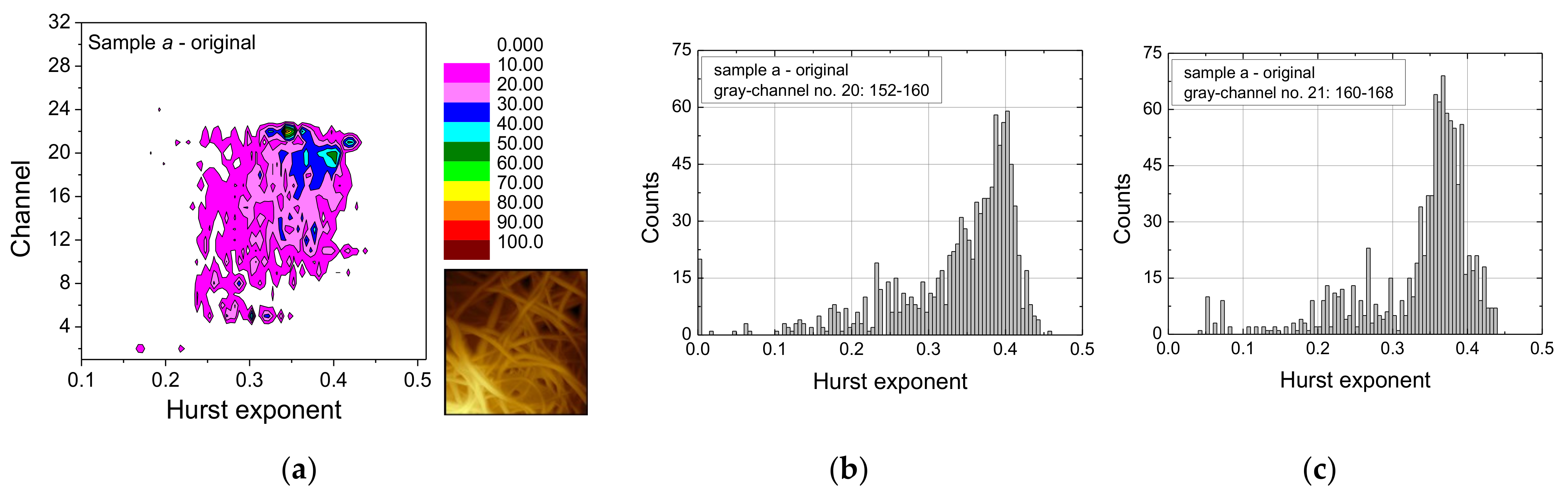
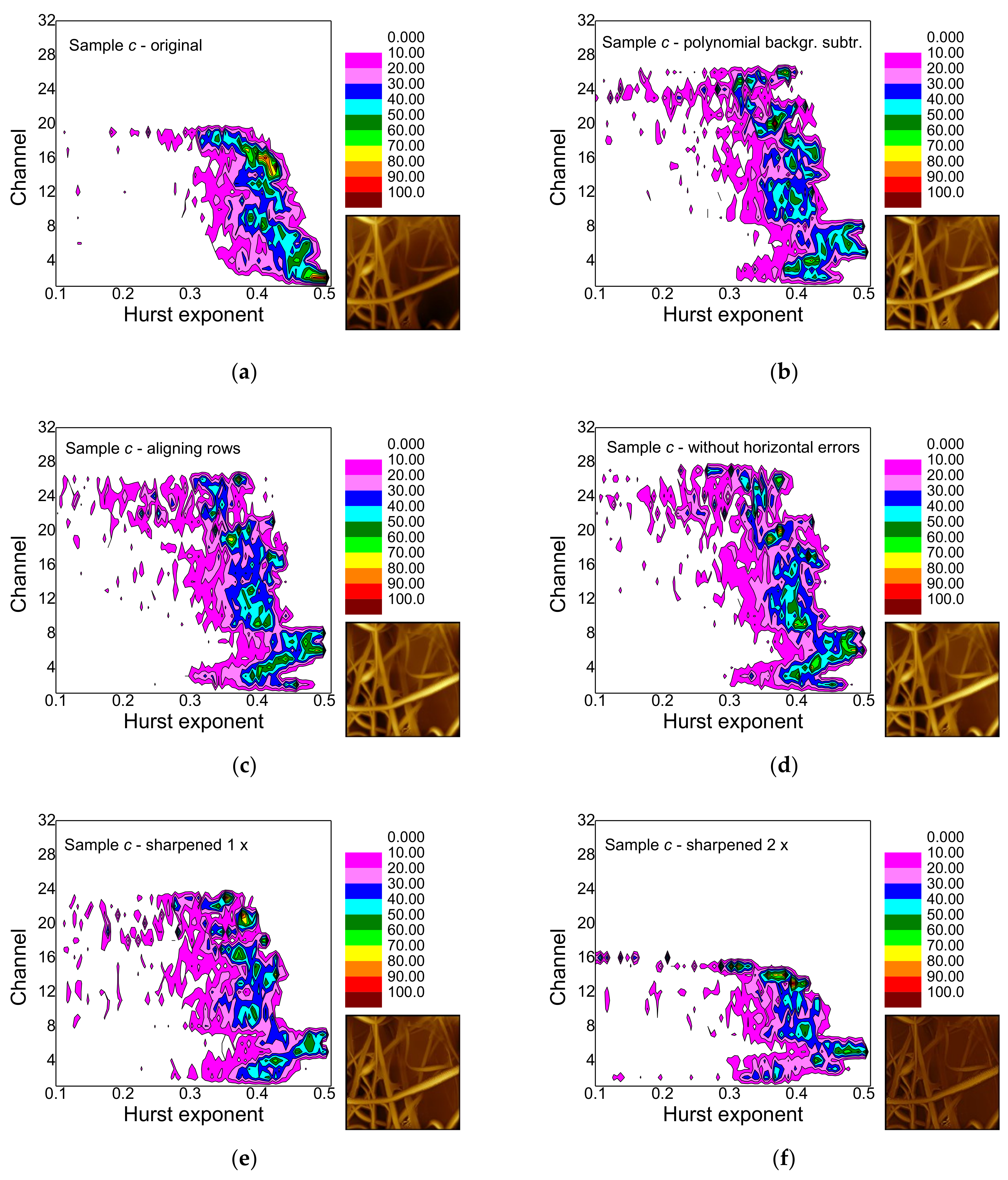
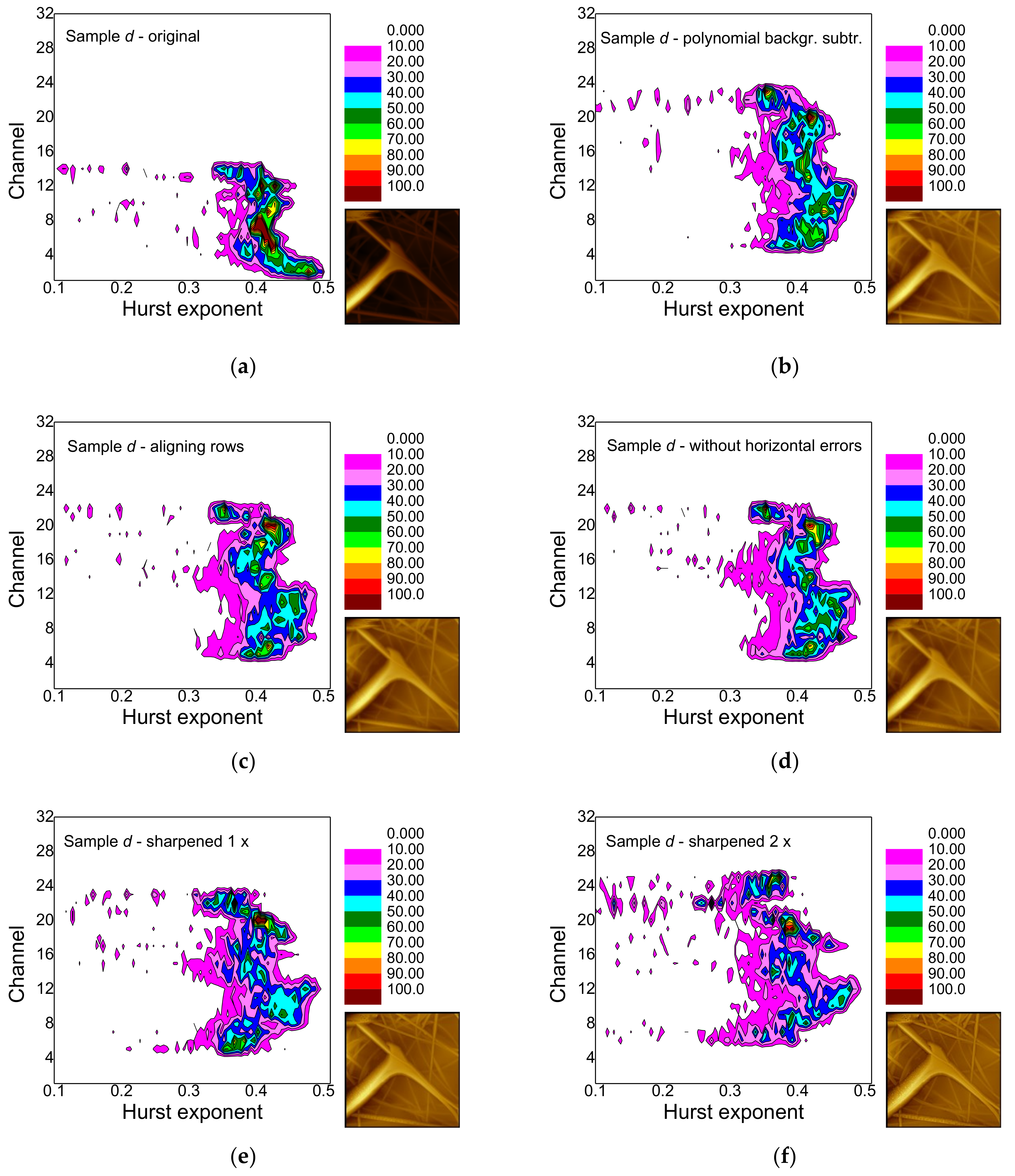
False-color maps of gray-scale-resolved Hurst exponent distributions enable distinguishing between different fiber distributions, especially between images with many and with only few fibers.

-

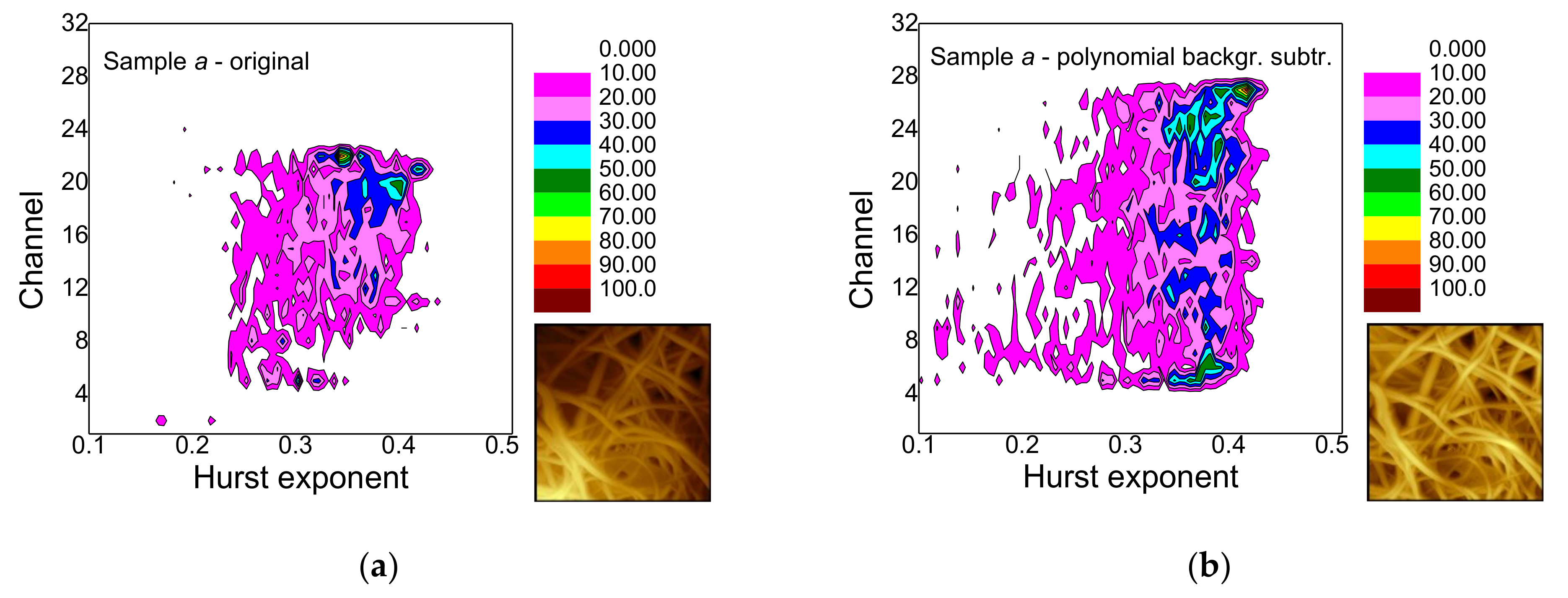
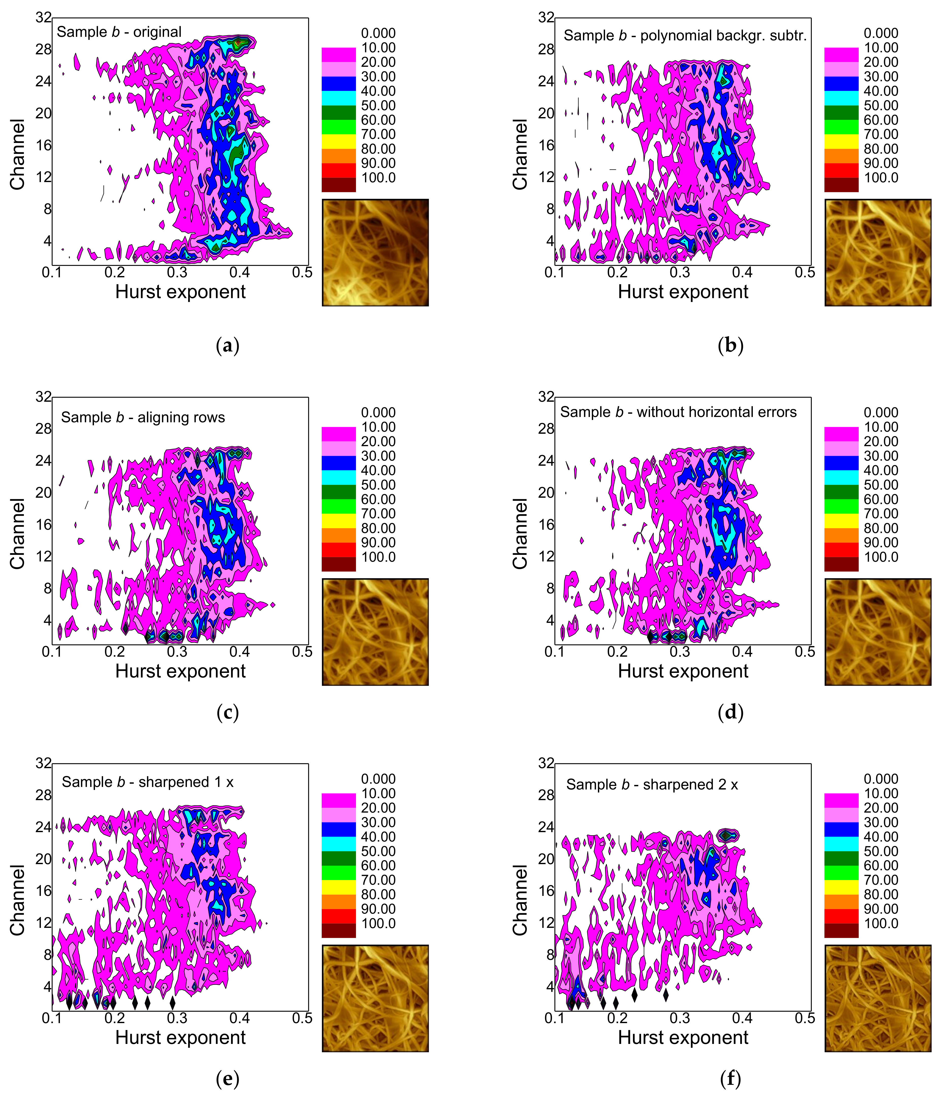
Polynomial background subtraction levels out the upper channel numbers for which a signal occurs and should thus be performed, especially in order to avoid ignoring hidden features (cf. Figure 9a,b).

-

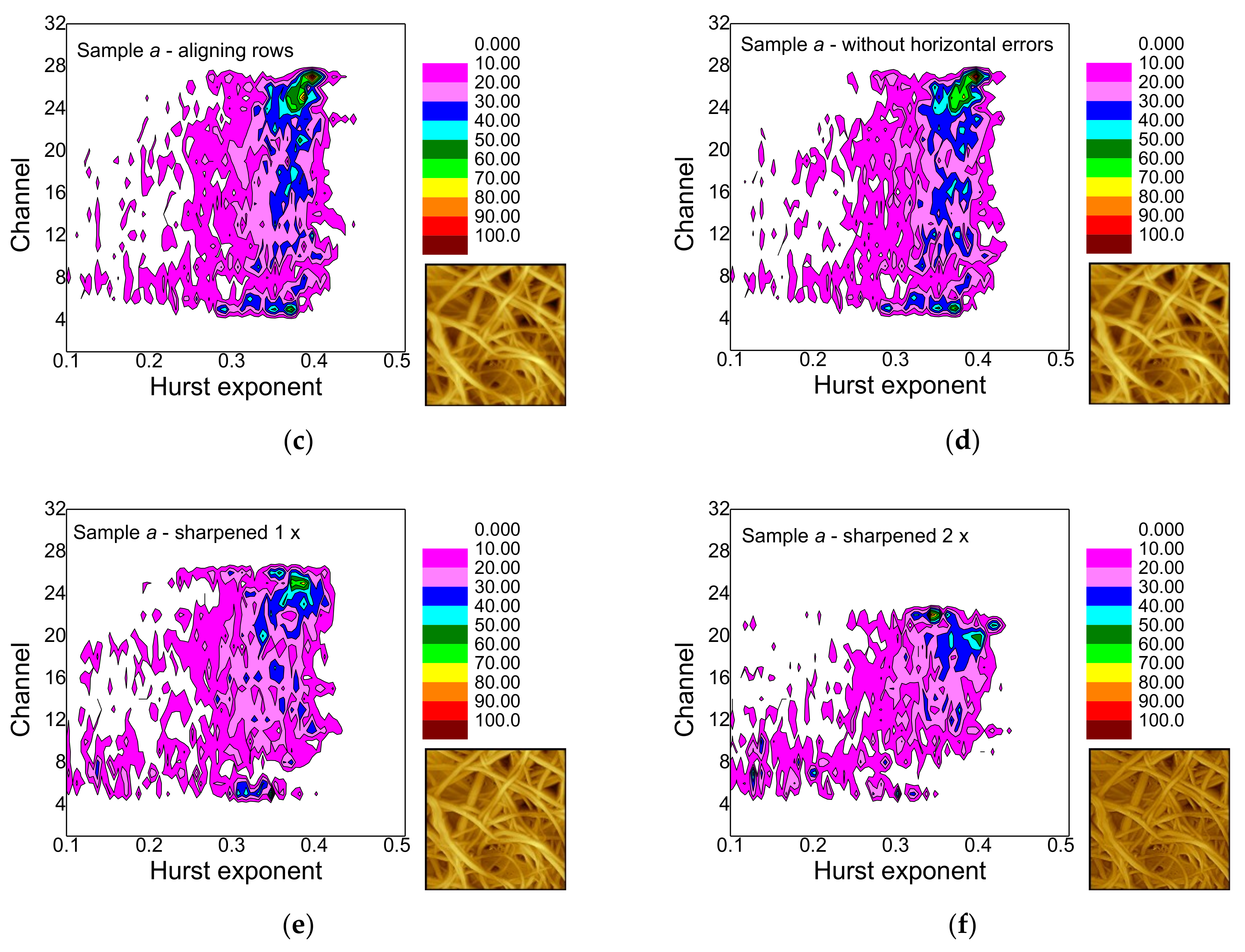
Aligning rows and deleting horizontal errors leaves the images and thus, the false-color maps nearly unaltered.

-

The effect of sharpening once differs from sample to sample and must be investigated further in the next study.

-

Sharpening twice modifies not only the image in an unnaturally looking way, but also the false-color maps of the gray-scale-resolved Hurst exponent distributions and should thus be avoided.

-

What could not be performed yet, but has to be tested in the near future, is a comparison with a highly accurate AFM with increased quality of the original images, as reported in [36].

-

Generally, the meaning of the “noise” in the range of Hurst exponents values below approx. 0.25 needs further investigation to find out whether this range should be ignored since it is mostly based on errors in the images, or whether it can oppositely be used as part of the “fingerprint” of such AFM images. To explain the threshold value of 0.25, we can refer to the composition of two random processes in analogy to [37]. In our model the first random process would concern the formation of tiny features in textiles (or their maps) and the second one would be the random walk itself. Further referring to [25], such Hurst exponent values (being the inverse of the fractal dimension of the random walk therein) would be far below the outcome of the random walk on any percolation model in 2D.

4. Conclusions

AFM images were evaluated by gray-scale-resolved Hurst exponent distributions, based on random walks on monochromatic maps prepared according to the gray-scale distributions. In this way, we propose a new indicator of microscopic images enabling characterization of graphical information equivalent to different scales and sizes. Meaningful signals in the range of Hurst exponent values up to approx. 0.25 indicate small (local) features, while larger Hurst exponent values are correlated with larger (more global) areas. Our investigation also demonstrates that post-processing methods can support image evaluation according to Hurst exponent distributions, such as the polynomial background subtraction, or reduce the information given by the gray-scale-resolved Hurst exponent distributions, such as a second sharpening step.

Future examinations will concentrate on investigating the effect of sharpening once, as well as on the meaning of the signals in the range of Hurst exponent values below approx. 0.25. For now, we can refer to the fact that a Hurst exponent value of 0.25 is far below the outcome of any percolation model in 2D; hence, it refers to the fragmented image (what is rather typical for tiny features). We also plan investigations of nonlinear (i.e., quadratic) random walks, in the sense scaling of traveled distances, when new effects associated with incomplete information might occur.

References

1. Maver, T.; Kurecic, M.; Pivec, T.; Maver, U.; Gradisnik, L.; Gasparic, P.; Kaker, B.; Bratusa, A.; Hribernik, S.; Stana Kleinschek, K. Needleless electrospun carboxymethyl cellulose/polyethylene oxide mats with medicinal plant extracts for advanced wound care applications. Cellulose 2020, 27, 4487–4508. [Google Scholar] [CrossRef]
2. Grothe, T.; Storck, J.L.; Dotter, M.; Ehrmann, A. Impact of solid content in the electrospinning solution on physical and chemical properties of polyacrylonitrile (PAN) nanofibrous mats. Tekstilec 2020, 63, 225–232. [Google Scholar]
3. Roche, R.; Yalcinkaya, F. Electrospun polyacrylonitrile nanofibrous membranes for point-of-use water and air cleaning. ChemistryOpen 2019, 8, 97–103. [Google Scholar] [CrossRef]
4. Grothe, T.; Großerhode, C.; Hauser, T.; Kern, P.; Stute, K.; Ehrmann, A. Needleless electrospinning of PEO nanofiber mats. Adv. Eng. Res. 2017, 102, 54–58. [Google Scholar]
5. Reneker, D.H.; Chun, I.S. Nanometre diameter fibres of polymer, produced by electrospinning. Nanotechnology 1996, 7, 216–223. [Google Scholar] [CrossRef] [Green Version]
6. Lemma, S.M.; Esposito, A.; Mason, M.; Brusetti, L.; Cesco, S.; Scampicchio, M. Removal of bacterial and yeast in water and beer by nylon nanofibrous membranes. J. Food Eng. 2015, 157, 1–6. [Google Scholar] [CrossRef]
7. Boyraz, E.; Yalcinkaya, F.; Hruza, J.; Maryska, J. Surface-modified nanofibrous PVF membranes for liquid separation technology. Materials 2019, 12, 2702. [Google Scholar] [CrossRef] [PubMed] [Green Version]
8. Lin, K.-Y.A.; Yang, M.-T.; Lin, J.-T.; Du, Y.C. Cobalt ferrite nanoparticles supported on electrospun carbon fiber as a magnetic heterogeneous catalyst for activating peroxymonosulfate. Chemosphere 2018, 208, 502–511. [Google Scholar] [CrossRef]
9. García-Mateos, F.J.; Cordero-Lanzac, T.; Berenguer, R.; Morallón, E.; Cazorla-Amorós, D.; Rodríguez-Mirasol, J.; Cordero, T. Lignin-derived Pt supported carbon (submicron)fiber electro-catalysts for alcohol electro-oxidation. Appl. Catal. B Environ. 2017, 211, 18–30. [Google Scholar] [CrossRef]
10. Dalton, P.D.; Klinkhammer, K.; Salber, J.; Klee, D.; Möller, M. Direct in vitro electrospinning with polymer melts. Biomacromolecules 2006, 7, 686–690. [Google Scholar] [CrossRef] [PubMed]
11. Wehlage, D.; Blattner, H.; Sabantina, L.; Böttjer, R.; Grothe, T.; Rattenholl, A.; Gudermann, F.; Lütkemeyer, D.; Ehrmann, A. Sterilization of PAN/gelatin nanofibrous mats for cell growth. Tekstilec 2019, 62, 78–88. [Google Scholar] [CrossRef]
12. Mamun, A. Review of possible applications of nanofibrous mats for wound dressing. Tekstilec 2019, 62, 89–100. [Google Scholar] [CrossRef]
13. Wehlage, D.; Blattner, H.; Mamun, A.; Kutzli, I.; Diestelhorst, E.; Rattenholl, A.; Gudermann, F.; Lütkemeyer, D.; Ehrmann, A. Cell growth on electrospun nanofiber mats from polyacrylonitrile (PAN) blends. AIMS Bioeng. 2020, 7, 43–54. [Google Scholar] [CrossRef]
14. Bian, Y.; Wang, S.J.; Zhang, L.; Chen, C. Influence of fiber diameter, filter thickness, and packing density on PM2.5 removal efficiency of electrospun nanofiber air filters for indoor applications. Build. Environ. 2020, 170, 106628. [Google Scholar] [CrossRef]
15. Nikbakht, M.; Salehi, M.; Rezayat, S.M.; Majidi, R.F. Various parameters in the preparation of chitosan/polyethylene oxide electrospun nanofibers containing Aloe vera extract for medical applications. Nanomed. J. 2020, 7, 21–28. [Google Scholar]
16. Storck, J.L.; Grothe, T.; Mamun, A.; Sabantina, L.; Klöcker, M.; Blachowicz, T.; Ehrmann, A. Orientation of electrospun magnetic nanofibers near conductive areas. Materials 2020, 13, 47. [Google Scholar] [CrossRef] [PubMed] [Green Version]
17. Zheng, G.F.; Jiang, J.X.; Wang, X.; Li, W.W.; Liu, J.; Fu, G.; Lin, L.W. Nanofiber membranes by multi-jet electrospinning arranged as arc-array with sheath gas for electrodialysis applications. Mater. Des. 2020, 189, 108504. [Google Scholar] [CrossRef]
18. Gaalova, J.; Yalcinkaya, F.; Curinova, P.; Kohout, M.; Yalcinkaya, B.; Kostejn, M.; Jirsak, J.; Stibor, I.; Bara, J.E.; van der Bruggen, B.; et al. Separation of racemic compound by nanofibrous composite membranes with chiral selector. J. Membr. Sci. 2020, 596, 117728. [Google Scholar] [CrossRef]
19. Bu, H.G.; Huang, X.B. A novel multiple fractal features extraction framework and its application to the detection of fabric defects. J. Text. Inst. 2008, 99, 489–497. [Google Scholar] [CrossRef]
20. Conci, A.; Proenca, C.B. A fractal image analysis system for fabric inspection system based on box counting method. Comput. Netw. Isdn Syst. 1998, 30, 1887–1895. [Google Scholar] [CrossRef]
21. Giorgilli, A.; Casati, D.; Sironi, L.; Galgani, L. An efficient procedure to compute fractal dimensions by box counting. Phys. Lett. A 1986, 115, 202–206. [Google Scholar] [CrossRef]
22. Valous, N.A.; Mendoza, F.; Sun, D.-W.; Allen, P. Texture appearance characterization of pre-sliced pork ham images using fractal metrics: Fourier analysis dimension and lacunarity. Food Res. Intern. 2009, 42, 353–362. [Google Scholar] [CrossRef]
23. Plotnick, R.E.; Gardner, R.H.; Hargrove, W.W.; Prestegaard, K.; Perlmutter, M. Lacunarity analysis: A general technique for the analysis of spatial patterns. Phys. Rev. E 1996, 53, 5461–5468. [Google Scholar] [CrossRef] [Green Version]
24. Grzybowski, J.; Blachowicz, T. Estimation of spatial distribution and symmetry of textile materials using numerical classification. Commun. Dev. Assem. Text. Prod. 2020, 1, 180–185. [Google Scholar] [CrossRef]
25. Havlin, S.; Ben-Avraham, D. Diffusion in disordered media. Adv. Phys. 2002, 51, 187–292. [Google Scholar] [CrossRef]
26. Haus, J.W.; Kehr, K.W. Diffusion in regular and disordered lattices. Phys. Rep. 1987, 150, 263–406. [Google Scholar] [CrossRef]
27. Li, J.; Teng, H.L.; Liu, S.Q.; Xu, J.; Li, T.D. Three-dimensional spatial distribution analysis of fibre in wet-blue pig leather. J. Soc. Leather Technol. Chem. 2018, 102, 111–117. [Google Scholar]
28. Blachowicz, T.; Ehrmann, A.; Domino, K. Statistical analysis of digital images of periodic fibrous structures using generalized Hurst exponent distributions. Phys. A Stat. Mech. Appl. 2016, 452, 167–177. [Google Scholar] [CrossRef]
29. Ehrmann, A.; Blachowicz, T.; Domino, K.; Aumann, S.; Weber, M.O.; Zghidi, H. Examination of hairiness changes due to washing in knitted fabrics using a random walk approach. Text. Res. J. 2015, 85, 2147–2154. [Google Scholar] [CrossRef]
30. Ehrmann, A.; Blachowicz, T.; Zghidi, H.; Weber, M.O. Reliability of statistic evaluation of microscopic pictures taken from knitted fabrics. J. Phys. Conf. Ser. 2015, 633, 012101. [Google Scholar] [CrossRef] [Green Version]
31. Blachowicz, T.; Böhm, T.; Grzebowski, J.; Domino, K.; Ehrmann, A. Analysis of AFM images of nanofibre mats for automated processing. Tekstilec 2020, 63, 104–112. [Google Scholar] [CrossRef]
32. Babič, M.; Kokol, P.; Guid, N.; Panjan, P. A new method for estimating the Hurst exponent H for 3D objects. Mater. Tehnol. 2014, 48, 203–208. [Google Scholar]
33. Matej, B.; Miliaresis, G.C.; Matjaž, M.; Ambu, R.; Michele, C. New method for estimating fractal dimension in 3d space and its application to complex surfaces. Int. J. Adv. Sci. Eng. Inf. Technol. 2019, 9, 2154–2159. [Google Scholar]
34. Blachowicz, T.; Andreychouk, V. Quantitative estimation of 3D cave networks complexity using random walk analysis. Landf. Anal. 2015, 29, 91–96. [Google Scholar] [CrossRef]
35. Ehrmann, A.; Blachowicz, T. Image processing techniques for evaluation of textile materials. In Examination of Textiles with Mathematical and Physical Methods; Springer International Publishing AG: Cham, Switzerland, 2017; pp. 89–112. [Google Scholar]
36. Mokrvenaite-Vilkonciene, I.; Virzonis, D.; Dzedzickis, A.; Bucinskas, V.; Rozene, J.; Vilkoncius, R.; Vaiciulis, D.; Ramanaviciene, A.; Ramanavicius, R. The improvement of the accuracy of electromagnetic actuator based atomic force microscope operating in contact mode and the development of a new methodology for the estimation of control parameters and the achievement of superior image quality. Sens. Act. A Phys. 2019, 287, 168–176. [Google Scholar] [CrossRef]
37. Gadomski, A. Multilineal random patterns evolving subdiffusively in square lattice. Fractals 2003, 11, 233–241. [Google Scholar] [CrossRef]
Figure 1. Original atomic force microscopy (AFM) images (ad), taken on different positions of an electrospun nanofiber mat, as explained in detail in the text.
Applsci 11 02436 g001
Figure 2. Post-treatment steps, performed on sample a: (a) polynomial background subtraction; (b) aligning rows; (c) deleting horizontal errors; (d) sharpening once.
Applsci 11 02436 g002
Figure 3. Gray-scale distribution (excerpt) of Figure 2a: (a) channels 32–39; (b) channels 104–111; (c) channels 112–119; (d) channels 208–215. Comparing with Figure 2a, one can conclude that (a) is connected with deepest features that are darkest, while (d) is correlated with the top features that are brightest; hence, the gray scale reflects the 3D structure of the image.
Applsci 11 02436 g003
Figure 4. Example of the random walks evaluation on AFM gray-scale-resolved images: (a) linear relation between ln ( Δ r 2 and ln(n); (b) Hurst exponent distribution.
Applsci 11 02436 g004
Figure 5. (a) Gray-scale-resolved Hurst exponent distribution of sample a in the original version, with the color-code giving the counts of the included histograms; (b) classical distribution for channel 20; classical distribution for channel 21 (c).
Applsci 11 02436 g005
Figure 6. Gray-scale-resolved Hurst exponent distribution of sample a: (a) original (identical to Figure 5a); (b) after polynomial background subtraction; (c) after aligning rows; (d) after deleting horizontal errors; (e) after sharpening; (f) after sharpening twice.
Applsci 11 02436 g006aApplsci 11 02436 g006b
Figure 7. Gray-scale-resolved Hurst exponent distribution of sample b: (a) original; (b) after polynomial background subtraction; (c) after aligning rows; (d) after deleting horizontal errors; (e) after sharpening; (f) after sharpening twice.
Applsci 11 02436 g007
Figure 8. Gray-scale-resolved Hurst exponent distribution of sample c: (a) original; (b) after polynomial background subtraction; (c) after aligning rows; (d) after deleting horizontal errors; (e) after sharpening; (f) after sharpening twice.
Applsci 11 02436 g008
Figure 9. Gray-scale-resolved Hurst exponent distribution of sample c: (a) original; (b) after polynomial background subtraction; (c) after aligning rows; (d) after deleting horizontal errors; (e) after sharpening; (f) after sharpening twice.
Applsci 11 02436 g009
Publisher’s Note: MDPI stays neutral with regard to jurisdictional claims in published maps and institutional affiliations.