Thermo-Economic Comparisons of Environmentally Friendly Solar Assisted Absorption Air Conditioning Systems

Abstract

Absorption refrigeration cycle is considered a vital option for thermal cooling processes. Designing new systems is needed to meet the increasing communities’ demands of space cooling. This should be given more attention especially with the increasing conventional fossil fuel energy costs and CO₂ emission. This work presents the thermo-economic analysis to compare between different solar absorption cooling system configurations. The proposed system combines a solar field, flashing tank and absorption chiller: two types of absorption cycle H₂O-LiBr and NH₃-H₂O have been compared to each other by parabolic trough collectors and evacuated tube collectors under the same operating conditions. A case study of 200 TR total cooling load is also presented. Results reveal that parabolic trough collector combined with H₂O-LiBr (PTC/H₂O-LiBr) gives lower design aspects and minimum rates of hourly costs (5.2 $/h) followed by ETC/H₂O-LiBr configuration (5.6 $/h). H₂O-LiBr gives lower thermo-economic product cost (0.14 $/GJ) compared to the NH₃-H₂O (0.16 $/GJ). The absorption refrigeration cycle coefficient of performance ranged between 0.5 and 0.9.

1. Introduction

Today, the substitution of traditional energy sources by renewable ones has becomes urgently needed for the clean and sustainable development of the energy sector worldwide. Climate change, the world’s noticeable growth in population number, and the improvement in standard conditions of living make cooling demands to increase significantly. According to the International Institute of Refrigeration reports, approximately 15% of total electricity production in the world is used for refrigeration and air conditioning [1]. About 80% of the global electricity is produced from fossil fuels, which increases the emissions of greenhouse gases significantly [2]. Solar thermally activated cooling systems are more attractive than the other type because of the near concurrence of peak cooling loads with the available solar power. Taking into account the deficiency in electrical power in most developing countries, all these previous factors make solar cooling technology a suitable and clean alternative for a big problem. Current studies of solar thermal cooling technology should strive to realize modern, low-cost, energy-efficient, high-temperature collectors, and to develop a high-performance, low-temperature enabled air conditioning technology [3]. In particular, there has to be a determination to find the optimal operational capabilities that make the optimum total performance of the device to be reached despite the apparent specific use of high-efficiency technology. Today, absorption chillers are the most mature technology. Therefore, solar thermal absorption cooling units might be a great option to reduce the usage of electricity in cooling and obtain economic gains [4,5,6].

There are different technologies to produce cold (cooling of industrial processes, conservation of products, air conditioning, etc.) with solar energy (and with solar thermal energy in particular). Syed et al. [7] performed a simple economic analysis comparing eight different configurations of solar cooling systems. These configurations contemplated reasonable combinations of refrigeration (ejector, compression, and absorption) and solar electric drive (with photovoltaic collectors) or thermal drive (flat plate collectors FPC, evacuated tube collector ETC, and parabolic through collector PTC). They concluded that solar thermal systems using absorption refrigeration are the most economical; in particular those with low temperature (flat collectors coupled with single-effect absorption), solar collectors account for the highest life cycle costs in all the configurations analyzed.

In the solar thermal sector, the main technologies integrated with absorption cooling systems are FPC, ETC, and PTC [8]. Parabolic through collectors have been analyzed in many types of research through single impact absorption cycles. Li et al. [9] inspected experimentally the performance of this configuration for Kunming, China, and they concluded that 56 m² of PTCs can drive H₂O-LiBr absorption cycle with 6 TR cooling capacity to serve the cooling requirements of a meeting room of 102 m². Besides this, they analyzed appropriate methods for improving cooling performance. In Iran, Mazloumi et al. [10] proved that 57.6 m² of PTC, storage tank of 1.26 m³ equipped with absorption system can satisfyingly meet building cooling load. The system operated from 6:00 to 19:00.

Shirazi et al. [11] compared three configurations of H₂O-LiBr solar absorption cooling system with TRNSYS 17. The first one was a single effect absorption integrated with ETC. The second and third configurations were double and triple effect systems, respectively, with PTC. The results revealed that the use of multi-effect absorption solar cycles was not advantageous over single-effect solar systems when the fraction of direct normal irradiation is less than 60% of the total global solar irradiation. Furthermore, the analysis of cost results indicated that a fraction of minimum direct normal irradiation of about 70% was required for solar-powered multi-effect cooling systems in order to be cost-effective in comparison to single-effect solar cooling systems.

The use of ETC to provide refrigeration in Saudi Arabia has been examined by Khan et al. [12], and they demonstrated that the use of 116 m² of ETC can lead to satisfying results with 10 kW cooling capacity of NH₃–H₂O absorption refrigeration system.

Rajasekar et al. [13] examined a single effect NH₃-H₂O chiller of one KW, which was using an evacuated tube solar collector. They deduced that the optimum coefficient of performance (COP) was accomplished at the temperature of the generator of 83.2 °C and while the evaporator temperature was 23.59 °C. A comparison was achieved among their accomplished COP values with standard absorption solar cooling systems.

Flores et al. [14] compared the operation of the absorption cooling system with different working pairs and presented a computer program to study H₂O-LiBr, NH₃-H₂O, and the other four pairs’ performance. They found that due to crystallization problems, the H₂O-LiBr pair operates at a small range of vapor temperature operation specifically at generator temperature of 75–95 °C. In the case of the NH₃-H₂O system, the range of generator temperature was 78–120 °C. The condenser, evaporator, and absorber temperatures were 40 °C, 10 °C, and 35 °C, respectively, for a cooling load of 1 kW for each working pair.

Many researchers have carried out exergetic analysis studies for different thermal solar absorption cooling systems. Gebreslassie et al. [15] studied an exergy analysis for all components in the absorption cycle. They found that the largest exergy destruction occurs at the absorbers and generators. In the same regard, Kilic et al. [16] utilized the first and second laws of thermodynamics to develop a mathematical model for single stage H₂O-LiBr refrigeration cycle and they proved that the system COP increases with the increase of generator and evaporator temperature, while system COP decreases as condenser and absorber temperature increases. In the same regard, Ahmet Karkas et al. [17] carried out energy analysis for absorption cooling cycles and states that, above 0 °C, the cycles of H₂O-LiBr cooling are more effective based on thermodynamics laws. Dincer et al. [18] investigated procedures of calculating the total exergy, both chemical and physical exergy for the absorption cooling system, using the realization of a series of programming algorithms, with the help of the correlations supplied in the Engineering Equation Solver (EES).

Related to thermo-economics, Lu and Wang [19] analyzed economically three types of solar cooling systems. The first one was an adsorption system integrated with ETC solar collector the cycle employing water and silica gel as a working solution. The second system was a single-effect (H₂O-LiBr) absorption system connected by an efficient compound parabolic concentrating solar collector. Finally, the last system was a double-effect (H₂O-LiBr) absorption cycle equipped with PTC. They deduced that the third system had the highest solar coefficient of performance (COP). They also concluded that the cooling chiller can be driven at an ambient temperature of 35 °C from 14:30 to 17:00.

In recent years, the studies that have contributed to the improvement of the performance of absorption systems are related to hybrid absorption. Colorado and Rivera [20] have compared various refrigeration systems by vapor compression with a hybrid system(compression/absorption) based on the 1st and 2nd laws of thermodynamics; in the compression cycle, they utilized R134a and CO₂ as refrigerants, and for absorption cycle, they used H₂O-LiBr as an operating mixture. The hybrid system has a cascade heat exchanger, in this case, the condenser of the compression cycle is considered the evaporator of the absorption cycle. The study aims to enhance the efficiency and reduce the energy consumption in the compressor. The research results show that the hybrid system consumes 45% less electricity than the simple compression cycle. Likewise, the coefficient of performance (COP) achieved with the hybrid system was higher with R134a refrigerant.

A major benefit of the absorption cooling system is the opportunity to use different heat sources to drive the generator of absorption. Wang et al. [21] investigated the optimal heat sources for different absorption cooling system applications. The heat released from the exhaust gases of boilers, internal combustion engines, and gas turbines could be utilized as a heat source for an absorption system. Du et al. [22] constructed a prototype of a single-stage NH₃-H₂O cooling system that operated with a heat discarded from a diesel engine through an active open-pipe heating method, which was designed to provide a uniform amount of available heat. The authors designed the heat exchanger to recover energy discarded for a specific capacity, combining the processes of condensation and absorption in a refrigeration unit by circulating a solution that had been previously cooled.

Finally, two latest thermo-economic comparative studies by authors in this field need to be mentioned [23,24], which compared the use of ETC and PTC integrated with H₂O-LiBr and/or NH₃-H₂O absorption chiller energetically and financially. They found that, generally, PTC in both cases (PTC-H₂O-LiBr/NH₃-H₂O) is the best option with large capacities and the use of (ETC-H₂O-LiBr/NH₃-H₂O) as a next alternative.

The previous literature review states that there are a lot of investigations on thermal absorption cooling systems field and most of them deal with LiBr-H₂O or H₂O-NH₃ as working pairs, and that most of them used traditional absorption cycles. Numerous ideas on thermodynamic and economic studies are being examined. In general, for each comparative research, only one technique was investigated. In this direction, this work is a comparative analysis of four common solar thermal cooling systems. More specifically, it compares the use of two kinds of collectors (ETC and PTC) for the solar part and the absorption cycles H₂O-LiBr and NH₃-H₂O with each other under the same operating conditions.

The innovation of this work has arisen from the method of combination of solar field and absorption cycle by using flash tank as the investigated thermal enhancement method. To the authors’ knowledge, no article available in literature has dealt with the proposed integration from that side, and in general, comparative researches are restricted. Therefore, this work is innovative because it systematically presents a comparison between four configurations. The solar cooling plant introduced in this work is suitable for medium and high loads of cooling. This may be reasonable for coastal and tourist spots along with the solar beam areas like the Middle East, North Africa (MENA), and Gulf regions.

The main objective of this work is to improve and compare between the various configuration of absorption refrigeration cycles by various solar thermal collectors. In this sense, steady-state energetic, exergetic, cost, and design techniques of modeling are performed for an absorption cooling system powered by solar energy. The optimal operating condition of the system is reported as well. The following outlines were withdrawn in this work:

• Two different types of absorption cycles in different working conditions were studied. The selection process involved the optimum operating conditions.
• Comparison was made of two different types of solar thermal collectors when combined with an absorption chiller.
• The mathematical model has been carried out in detail.
• The comparison was performed based on the terms of energy, exergy, design, cost, and thermo-economic. Design technique of modeling has been adopted in this study.
• Based on the optimized selection, a detailed case study was performed for a cooling load of 700~800 kW.

2. System Description

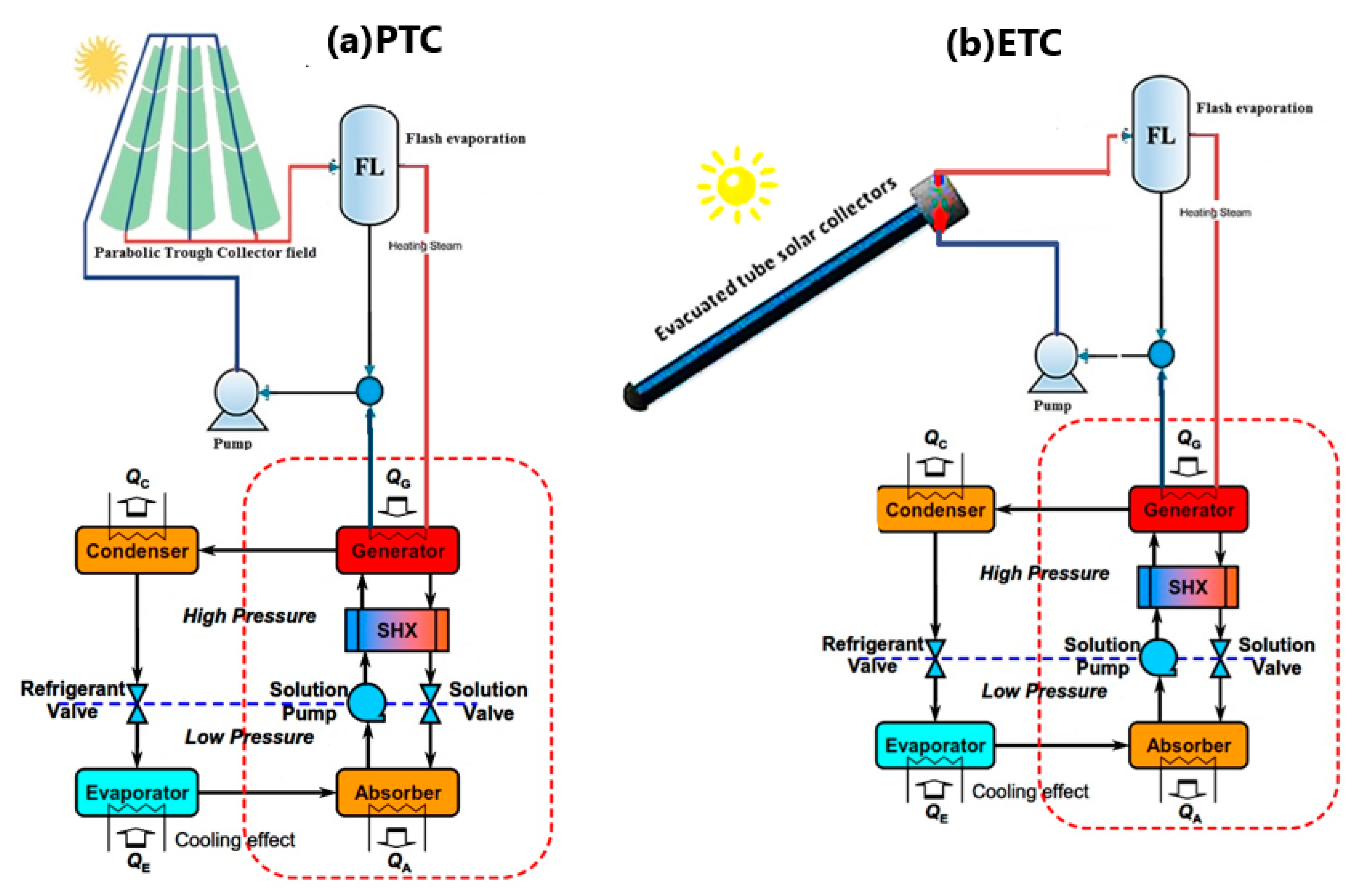
As mentioned previously, the proposed system combines two systems: a solar power system and an absorption air conditioning (AAC) system. The solar power system includes a thermal solar collector and flash tank. Basically, the plant is driven by solar energy. The current proposed absorption cooling systems (H₂O-LiBr/NH₃-H₂O) integrated with (PTC/ETC) are displayed in Figure 1.

Solar field loop combines a set of PTCs or ETCs. Water is employed as a working fluid. Solar radiation is collected and concentrated on the water by solar collectors. In simulation, solar intensity is assumed to be constant to accomplish the steady-state condition. Subsequently, the water with high temperature enters the flash tank to generate steam, and the condensed water is collected in the bottom of the flash tank and then back to the solar collector’s field via the heat release. The AAC unit is a single-stage H₂O-LiBr or NH₃-H₂O type. Flash tank steam condensation in the AAC generator results in the boiling of the solution and separation of the refrigerant (water or ammonia vapor). At the generator outlet, there is a two-phase flow. The steam phase involves the vapor of the refrigerant, which moves forward into a condenser unit; the liquid phase is a mixture (absorbent-refrigerant) with a low concentration of refrigerant (strong solution). Then, this solution is returned through a throttle valve to the absorber. In the AAC condenser, heat is removed from the refrigerant to the cooling water. The refrigerant is then throttled to fulfill the required temperature at the evaporator in which the chilled water acquires its low temperature needed for the cooling application. Besides this, the heat transfer results in a change in the thermodynamic state of the refrigerant from a saturated mixture of liquid and vapor to superheated vapor. The evaporated refrigerant is cooled, condensed, and mixed with the LiBr or water in the absorber forming a dilute solution. The refrigerant-absorber mixture causes an exothermic reaction, whereby the heat released in this process is discharged from the solution to the other stream via cooling water delivered from the secondary cooling system (air or cooling tower). The absorption process results in a mass flow of diluted solution leaving the absorber. Finally, the dilute solution is pumped back to the generator and so on. To enhance the AAC performance, strong and weak solutions exchange heat through a liquid-liquid heat exchanger. The utilization of the economizer increases the coefficient of performance (COP) by reducing heat released into the absorber and heat delivered to the generator. COP of a single effect system is defined as the relationship between the heat flow eliminated in the evaporator (cooling capacity) vs. the heat flow into the generator and the energy consumption of the pump. The single effect is represented by the basic absorption cycle, half effect, double effect, triple, and multi-effect absorption cycles. The term “effect” refers to the times that the driving heat is used by the absorption system, and the number of generators refers to the number of effects.

3. Methodology, Design Development Software, and Assumptions

The design of an absorption air conditioning cycle (AAC) requires a considerable amount of calculation. This makes it an extremely complex, cumbersome, and time-consuming process. That is why we chose to use software that facilitates it. MATLAB is a powerful software package for scientific computing, focusing on numerical calculations, matrix operations, and especially the applications of science and engineering. It can be used as a simple matrix calculator, but its main interest lies in the hundreds of functions—both general purpose and specialized—that it has, as well as its possibilities for graphic visualization.

In this work, the four configurations proposed model was coded in the MATLAB program, which allows you to establish a numerical method for solving the proposed model and makes it possible to solve the mathematical model of the simulator and provide the obtained results. Since it is a platform that allows making sequences of mathematical calculations, it is possible to model physical phenomena in the form of equations. In order to build the simulator, it is necessary to enter the equations with their respective nomenclatures and establish the criteria to be followed for the resolution of the sequence of steps. The origin of the physical characteristics is taken from the NIST chemistry book on their website [25]. More information about the optimization techniques considered in this work is given in Refs. [23,24], to minimize techno-economic costs.

Table 1. Design data for the solar absorption system configurations [24].

Unit Process	Assigned Data	Calculated Data
Absorption air-conditioning cycle (AAC)/(ETC/PTC)	✓ Solar radiation: 500 W/m2 ✓ Ambient temperature: 25 °C ✓ Average relative humidity: 15% ✓ ETC top temperature: 100–200 °C ✓ PTC top temperature: 200–300 °C ✓ Absorber temperature: 30–35 °C ✓ Generator temperature: 80–90 °C ✓ Condenser temperature: 40–45 °C ✓ Hot air temperature: 35 °C ✓ Target cooled air temperature: 20 °C ✓ Evaporator temperature: 5–10 °C ✓ Cooling load: 176–700 kW (50–200 TR) ✓ Condenser effectiveness: 80% ✓ Fan system efficiency: 85% ✓ Pumping system efficiency: 75% ✓ Plant life time: 20 years ✓ Interest rate: 5% ✓ Load factor: 90% ✓ Specific electric power cost: 0.065 $/kWh ✓ Water steam is the solar field working fluid	Solar Field: ➢ Solar field top pressure, bar ➢ Solar field pressure loss, bar ➢ Total solar field area, m2 ➢ Solar field thermal load, kW ➢ Number of solar collectors, # ➢ Solar field mass flow rate, kg/s ➢ Solar field inlet temperature, °C ➢ Efficiency, % ➢ Exergy destruction, kW Flash Tank: ➢ * Flash tank design data ➢ Total mass flow rate, kg/s ➢ Dryness fraction, % ➢ Flash tank water flow rate, kg/s ➢ Steam flow rate, kg/s ➢ Exergy destruction, kW AAC Unit: ➢ Weak & strong solutions, kg/s ➢ * Design data ➢ Thermal power, kW ➢ Total cycle flow rate, kg/s ➢ Generator power, kW ➢ Cooling fan power, kW ➢ Coefficient of performance (COP) ➢ COPmax ➢ Relative performance ➢ Exergy destruction, kW Pump: ➢ Power, kW ➢ Outlet temperature, °C ➢ Exergy destruction, kW Cost & Performance: ➢ Units hourly costs, $/h ➢ Total hourly costs, $/h ➢ Total power, kW ➢ LPC, $/kWh ➢ Thermo-economic cost, $/GJ ➢ Total exergy destruction rate, kW
Notes:	▪ Data are run out based on steady-state operating conditions. ▪ Ambient temperature is fixed as 25 °C for all process runs. ▪ Solar radiation is fixed at 500 W/m2. ▪ * Design data means area, length, width, etc.

shows parameters considered for the simulation of the four different system proposed configurations. In simulation, solar intensity is assumed to be constant to accomplish the steady-state condition. In all the absorption cycles, the energy input was used in the form of steam. For the thermodynamic, exergetic, and cost analysis, the equations that were applied are described in the following sections.

4. Mathematical Model

The studied system components are modeled and simulated depending on both first and second laws of thermodynamics. As a first step in modeling this system, the study is implemented depending on steady state basis at a constant value of solar radiation intensity. An explanation of the mathematical model of each part is clarified in the following sub-sections.

4.1. ETC Modeling

An immediate efficiency of the ETC solar collector can be calculated by the solar irradiance, average collector temperature, and environmental temperature based on its characteristic curve. For ETC, the curve adopted is specified by Equation (1) [26,27].

$${\eta }_{etc}={\eta }_o-a_1\left(\frac{T_o-T_{amb}}{I_s}\right)-a_2{\left(\frac{T_o-T_{amb}}{I_s}\right)}^2.I_s$$

(1)

where, ${\eta }_{etc}$ is the ETC efficiency, ${\eta }_{\mathrm{o}}=0.665$, $a_1$ = 2.9 W/m². °C, $a_2$ = 0.0019 W/m². °C², $I_s$ is the solar flux (W/m²), $T_o$ is the exit top temperature of the collector (°C), and $T_{amb}$ (°C) is the ambient temperature. The thermal load of the collector $Q_{th}$ (kW) is calculated according to Equation (2).

$$Q_{th}=M_{col}^{.}\times C_p\times \left(T_o-T_i\right)$$

(2)

where, $M_{col}^{.}$ is the mass flow rate in kg/s.

The total surface area of the collector $A_t$(m²), is calculated from the equation of the energy balance of the collector as a dependency of the efficiency using:

$$A_t=\frac{Q_{th}}{{\eta }_{etc}\times I_s}$$

(3)

The aperture area of the ETC module A_etc, m², can be calculated as:

$$A_{etc}=D_t\times L_t\times NOT$$

(4)

where, $D_t$ and $L_t$ is the diameter and length of the tube in (m), respectively, and $NOT$ is the tube numbers of each module. The total number of ETCs, $NOC$ could be estimated from the following relation:

$$NOC=\frac{A_t}{A_{etc}}$$

(5)

The loops number $NOL$, area of the loop $A_{loop}$, and the length of each loop, $L_{loop}$ could be computed by allocating the hydraulic mass flow rate $M_{hyd}^{.}$, kg/s.

$$NOL=\frac{M_{col}^{.}}{M_{hyd}^{.}}$$

(6)

$$A_{loop}=\frac{A_t}{NOL}$$

(7)

$$L_{loop}=\frac{A_{loop}}{L_t}$$

(8)

4.2. PTC Modeling

For the medium-high temperature of PTCs, the relevant efficiency can be found in Equation (9) [27]:

$${\eta }_{ptc}={\eta }_o-a_{11}\left(T_o-T_{amb}\right)-a_{21}\left(\frac{T_o-T_{amb}}{I_s}\right)-a_{31}{\left(\frac{T_o-T_{amb}}{I_s}\right)}^2$$

(9)

where, $a_{11}$ = 4.5 × 10⁻⁶ 1/ °C, $a_{21}$ = 0.039 W/m². °C, $a_{31}$ = 3 × 10⁻⁴ W²/m². °C², ${\eta }_{\mathrm{o}}=0.75$.

The thermodynamic performance of a PTC is expressed as:

$${\eta }_{PTC}=\frac{Q_u}{A_{PTC}\times I_s}$$

(10)

where, ${\eta }_{PTC}$ is the collector thermal efficiency; Qu is the useful thermal power (W); $A_{PTC}$ is the aperture area of the collector (m²); and Is is the solar radiation (W/m²). Modifying Equation (10) results in Equation (11):

$$A_{PTC}=\frac{Q_u}{{\eta }_{PTC}\times I_s}$$

(11)

The ground area necessary for solar collector implementation, however, is larger than the collector’s aperture area. This value ranges from about three to four times the collector’s aperture area, due to the space between the collectors in addition to the space needed for the pipes and other system accessories. The useful thermal energy of the collectors can exist according to the following relationship:

$$Q_u=M_{col}^{.}\times \Delta h_{o-i}$$

(12)

Here, $\Delta$h is the enthalpy difference of through collector in kJ/kg, and $M_{col}^{.}$ is the mass flow rate in kg/s. The total length of PTC, $L_{PTC}$ is then calculated depending on the width of the collector $W_c$ (m) and the diameter of the glass envelope $D_{env}$ (m):

$$L_{PTC}=\frac{A_{PTC}}{W_c-D_{env}}$$

(13)

By identifying the total mass flow rate, which is estimated based on the load of the boiler heat exchanger, and assigning a hydraulic mass flow rate to be the input, the entire number of loops $N_{loop}$, area of the loop $A_{loop}$, the width of the loop $W_{loop}$, and the solar PTC’s number ($N_{PT{C}^{\prime }s})$ are calculated as follows:

$$N_{loop}=\frac{M_{col}^{.}}{M_{hyd}^{.}}$$

(14)

$$A_{loop}=\frac{A_{PTC}}{N_{loop}}$$

(15)

$$W_{loop}=\frac{A_{loop}}{L_m}$$

(16)

where, $L_m$ (m) is assigned as the length of the module.

$$N_{PT{C}^{\prime }s}=\frac{A_{PTC}}{L_m\left(W_c-D_{env}\right)}$$

(17)

Overall pressure drops $P_{tloss}$ are determined based on the major and minor drops over the length of the field. The general loss-equation is carried out as follows [28,29]:

$$P_{tloss}=N_{loop}\times \Delta P_{loop}$$

(18)

where,

$$\Delta P_{loop}=\frac{32\times f\times L_{loop}\times M_{hyd}^{.}{}^2}{\rho \times {\pi }^2\times D_t}$$

(19)

$D_t$ is the inner tube diameter(m).

$$f={\left[\left(1.82\times \log Re\right)-1.64\right]}^{-2}$$

(20)

$$Re=4\times \frac{M_{hyd}^{.}}{\mu \times \pi \times D_t}$$

(21)

4.3. Flash Tank Modeling

The design parameters of the cyclone flash tank have been derived in the following manner:

Tank inlet and outlet tube steam area $A_{t_i}$ is determined according to the velocity of steam $V_{st}$, m/s, and the density of vapor ${\rho }_v$, kg/m³:

$$A_{t_i}=\frac{M_{st}}{{\rho }_v\times V_{st}}$$

(22)

Tube diameter $D_t$ (m):

$$D_t={\left(\frac{A_{t_i}\times 4}{\pi }\right)}^{0.5}$$

(23)

Height of flash tank $H_{fst}$ (m) [29]:

$$H_{fst}=7.15\times D_t$$

(24)

Flash tank width $W_{fst}$ (m):

$$W_{fst}=3.5\times D_t$$

(25)

Flash tank total volume $Vo{l}_{fst}$ (m³):

$$Vo{l}_{fst}=\left(\frac{Pi}{4}\right)\times W_{fst}{}^2\times H_{fst}$$

(26)

The flashing enthalpy $h_{fsh}$ equals the fluid enthalpy that comes from the solar collector $h_{col}$, kJ/kg:

$$h_{fsh}=h_{col}$$

(27)

The flashing dryness fraction $X_{fsh}$ is used to quantify the amount of water within steam and it is estimated depending on the enthalpy of flashing $h_{fsh}$, liquid enthalpy $h_f$, (kJ/kg), and dry vapor enthalpy $h_g$ (kJ/kg):

$$X_{fsh}=\frac{h_{fsh}-h_f}{h_g-h_f}$$

(28)

The total mass flow rate $M_{total}$ (kg/s) and non-vaporized water $M_w$ (kg/s) were calculated using Equations (29) and (30), respectively:

$$M_{total}=\frac{M_{st}}{X_{fsh}}$$

(29)

$$M_w=\left(1-X_{fsh}\right)\times M_{total}$$

(30)

4.4. Pump Modeling

The work of the pump $W_p$, kW may be determined using the following relation [30]:

$$W_p=M_{total}\times \frac{\Delta P}{\rho }\times {\eta }_p$$

(31)

where, $\Delta P$ (kPa) represents the difference in total pressure and it is computed as:

$$\Delta P=P_{high}+P_{loss}$$

(32)

Outlet pump enthalpy $h_{po}$ (kJ/kg):

$$h_{po}=\left(\frac{W_p}{M_{total}}\right)+h_{pi}$$

(33)

4.5. Absorption Chiller Modeling

The absorption cycle was developed for a capacity of cooling and specific temperature ranges. Table 1 shows the input parameters considered for the simulation of the absorption chiller. The mathematical model that was developed for the study of single-effect absorption cycles is based on the theory reported by the authors [23,24]. The following assumptions are considered for analyzing absorption systems:

• Analysis is carried out in steady-state conditions.
• The refrigerant leaving the condenser is in a saturated liquid state.
• The refrigerant when leaving the evaporator is in the saturated vapor state.
• Temperature at the outlet of the absorber and the generator belong to mixing equilibrium and the conditions of separation, respectively.
• The pressure drops through the pipes and heat exchangers are negligible.
• The heat exchange among the system and the environment are negligible.

The thermodynamic analysis model of the absorption cycle components is done with the help of basic balances, mass balance, energy balance, and solution phase equilibrium, and the general formulation are listed as follows:

$${\displaystyle \sum }{m}_i-{\displaystyle \sum }{m}_o=0$$

(34)

$${\displaystyle \sum }{m}_i{x}_i-{\displaystyle \sum }{m}_o{x}_o=0$$

(35)

$${\displaystyle \sum }{m}_i{h}_i-{\displaystyle \sum }{m}_o{h}_o=0$$

(36)

where, $m ,x$, and h denote mass, concentration, and enthalpy for inlet (i) and outlet (o) of the component, respectively. The total energy balance for the absorption cycle is specified as follows:

$$Q_e+Q_g=Q_c+Q_a+W_p$$

(37)

where, $Q_e$ is the thermal load on the evaporator, kW; $Q_g$ is the heat added to the Generator, kW; $Q_c$ is the heat expelled from the condenser, kW; $Q_a$ is the absorber thermal power, kW; and $W_p$ represents the pump work, kW. For performance calculations, the COP is defined as follows:

$$COP=\frac{Q_e}{Q_g}$$

(38)

The max COP of the ideal cycle is given by:

$$CO{P}_{max}=\frac{\left(T_e+273.15\right)\times \left(T_g-T_a\right)}{\left(T_g+273.15\right)\times \left(T_c-T_e\right)}$$

(39)

The relative performance ratio $RPR$ can be estimated as:

$$RPR=\frac{COP}{CO{P}_{max}}$$

(40)

From the analysis thermodynamic, data are obtained to obtain thermo-physical properties and to dimension the system components.

4.6. Thermo-Economic Model

In this part, the proposed system is mathematically analyzed to be evaluated it using thermo-economic approach (exergy and cost). Thermo-economic is the branch of engineering that combines exergy analysis and cost principles to provide the system designer or operator with information not available through conventional energy analysis and economic evaluation. Thermo-economic balance for any unit is performed based on exergy and cost balances.

The availability (exergy) and cost have been estimated based on the formulas reported in Refs. [31,32,33,34,35]. The equation of availability for any system is a fixed point; a stable flow process with first and second thermodynamic laws can be applied. By ignorance of kinetic and potential energy alterations, the following equation can be used to describe the form of availability [31]:

$$A_2-A_1=A_q+A_w+A_{fi}-A_{fo}-I$$

(41)

where, $A_2-A_1=0$ is the change of availability without flow in a steady-state condition; $A_q={{\displaystyle \sum }}_J\left(1-T_{amb}/T_J\right)Q_J$ is the transfer of availability due to heat exchange among the control volume and its surroundings; $A_w=-W_{cv}+P_o\left(V_2-V_1\right)$ is equivalent to negative work value generated by the control volume $W_{cv}$. In certain instances, though, the control volume has a fixed volume; therefore, $A_w$ can be simplified, and $I=T_{amb}.S_{gen}$ is the destruction availability of the process. Flow availability is specified as $A_{fi,o}={{\displaystyle \sum }}_{i,o}{m}_{i.o}^{.}{a}_{fi,o}$. Hence, the general form in steady-state condition would become:

$$0=A_q+A_w+A_{fi}-A_{fo}-I$$

(42)

In a conventional economic evaluation, a balance of costs for the total system running in a steady state is established as following [32]:

$${{\displaystyle \sum }}_{out}{C}^{.}={{\displaystyle \sum }}_{in}{C}^{.}+Z^{IC\&OM}$$

(43)

where, $C^{.}$ is the rating of cost based on in and out streams, and $Z^{IC\&OM}$ are related to capital expenditure and operational and maintenance costs. In the calculation of exergy costs, a cost is identified for every exergy stream. Hence, for the incoming and outgoing matter streams that have attached exergy exchange rates $E_{i,o}^{.}$, power $W^{.}$, and the exergy exchange rate assigned to the heat release $E_q^{.}$, Equation (43) can be written as follows:

$$C_{i,o}^{.}=c_{i,o}{E}_{i,o}^{.}$$

(44)

$$C_w^{.}=c_w{W}^{.}$$

(45)

$$C_q^{.}=c_q{E}_q^{.}$$

(46)

where, $c_{i,o},w,q$ represent the average cost for each unit of exergy in (USD/kJ) for inlet (i), outlet (o), power (w), and energy (q) respectively. The following relationships are used to estimate the costs per hour:

For cost analysis, the amortization factor $A_f$ is computed depend on:

$$A_f=\frac{i.{\left(1+i\right)}^{LTp}}{{\left(1+i\right)}^{LTp}-1}$$

(47)

The collector’s estimated cost of investment $I{C}_{col} \left(\mathrm{USD}\right)$ is determined according to the area correlation given below:

$$I{C}_{col}=150\times A_{col}^{0.95}$$

(48)

The cost of operation and maintenance $OM{C}_{col}$ is then calculated (USD):

$$OM{C}_{col}=0.15\times I{C}_{col}$$

(49)

Total annual cost $TA{C}_{col}$ (USD/y) is considered to depend on the parameters of operation and maintenance costs and investment costs, as indicated below:

$$TA{C}_{col}=\left(I{C}_{col}+OM{C}_{col}\right)\times A_f$$

(50)

Hourly costs are calculated $Z_{col}$ (USD/h):

$$Z_{col}=\frac{TA{C}_{col}}{OH\times 365}$$

(51)

where, $OH$ is operating hours (h)

Flashing tank investment cost $I{C}_{fsh}$ (USD) is calculated according to the total volume of the tank $Vo{l}_{fst}$ correlation:

$$I{C}_{fsh}=\frac{Vo{l}_{fst}\times 6300}{3.8}$$

(52)

The total annual cost $TA{C}_{fsh}$ USD/y is measured by:

$$TA{C}_{fsh}=I{C}_{fsh}\times A_f$$

(53)

Hourly costs are calculated $Z_{fsh}$ (USD/h):

$$Z_{fsh}=\frac{TA{C}_{fsh}}{OH\times 365}$$

(54)

Absorption cycle investment cost $I{C}_{aac} \left(\mathrm{USD}\right),$ is estimated on the base of the correlation of total area as:

$$I{C}_{aac}=150\times A_{aac}^{0.8}$$

(55)

Total annual cost $TA{C}_{aac}$ (USD/y) is then estimated:

$$TA{C}_{aac}=I{C}_{aac}\times A_f,$$

(56)

Hourly costs are calculated $Z_{aac}$ (USD/h):

$$Z_{aac}=\frac{TA{C}_{aac}}{OH\times 365}$$

(57)

Pump investment cost $I{C}_p \left(\mathrm{USD}\right)$ It is estimated on pump power correlation:

$$I{C}_p=3500\times W_p^{0.47}$$

(58)

Total annual cost $TA{C}_p$ (USD/y) It is estimated on:

$$TA{C}_p=I{C}_p\times A_f$$

(59)

Hourly costs are calculated $Z_p$ (USD/h):

$$Z_p=\frac{TA{C}_p}{OH\times 365}$$

(60)

Total hourly costs $Z_{tot}$ (USD/hr) It is estimated on all parameters:

$$Z_{tot}=Z_{col}+Z_{fsh}+Z_{aac}+Z_p$$

(61)

Total Plant Costs $TPC$ (USD/y) is also identified based on the total annual costs for all units:

$$TPC=TA{C}_{col}+TA{C}_{fsh}+TA{C}_{aac}+TA{C}_p$$

(62)

The cumulative thermo-economic equation is determined based on the expense and exergy flow of the cycles (USD/GJ):

$$c_p=1000\times \left(\frac{\left(W_{tot}\times c_w\right)+\left(\frac{Z_{tot}}{3600}\right)}{E{x}_{fo}}\right)$$

(63)

where, $c_p$ is the thermo-economic product cost (USD/GJ), $c_w$ is the energy price in (USD/kWh) (~0.065), and $W_{tot}$ is the cycle power(kW), while $E{x}_{fo}$ is the exergy stream outlet from the system to the user (kW).

5. Results and Analysis

The purpose of the simulation study was to indicate which combination of the absorption cycle model and solar thermal collector provides the most accurate information in order to bring the cost down. The investigated unit has never been studied before. Therefore, no experimental data is available, but the complete design can be used for this study. The application of design data promises reliable results. A common problem for numerical studies of a large-scale system capacity is the lack of validation data. One approach to resolve this problem is the usage of very detailed models and special simulation tools. In this study, the detailed design data values from Table 1 were used for the simulation of the solar absorption cooling system.

5.1. Water-Lithium Bromide (H₂O-LiBr) Cycle Results

5.1.1. Effect of Top Solar Field Temperature

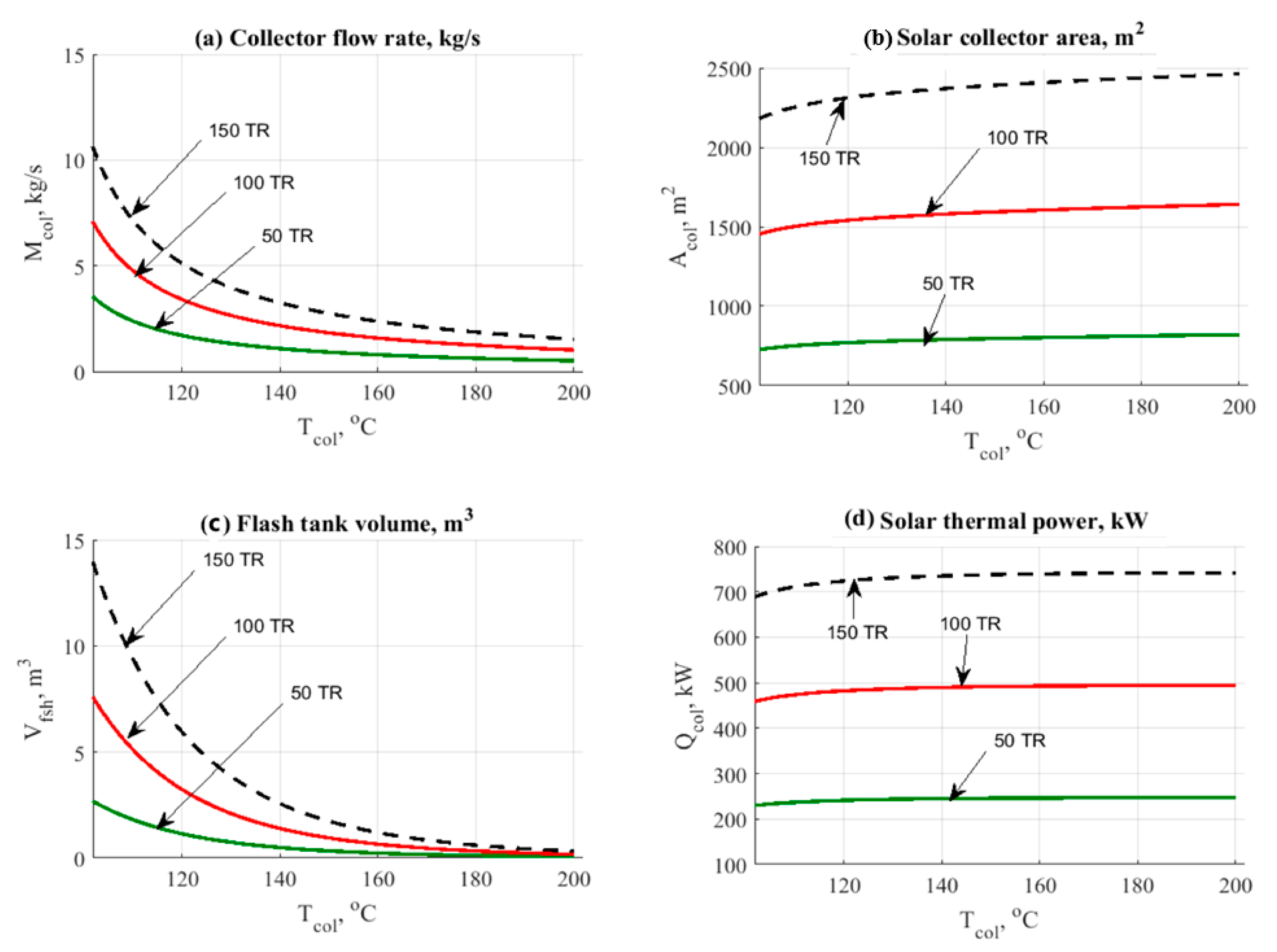
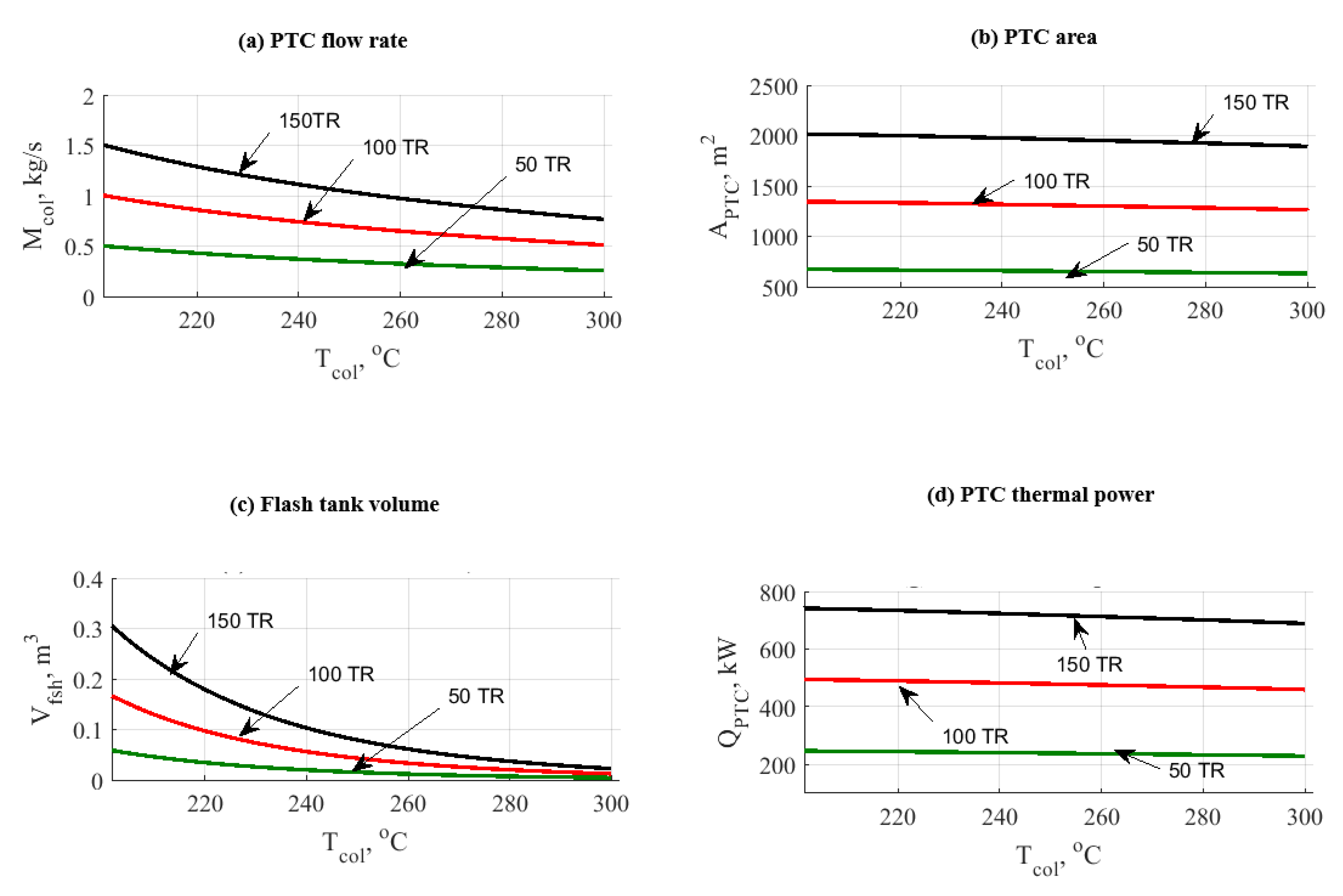
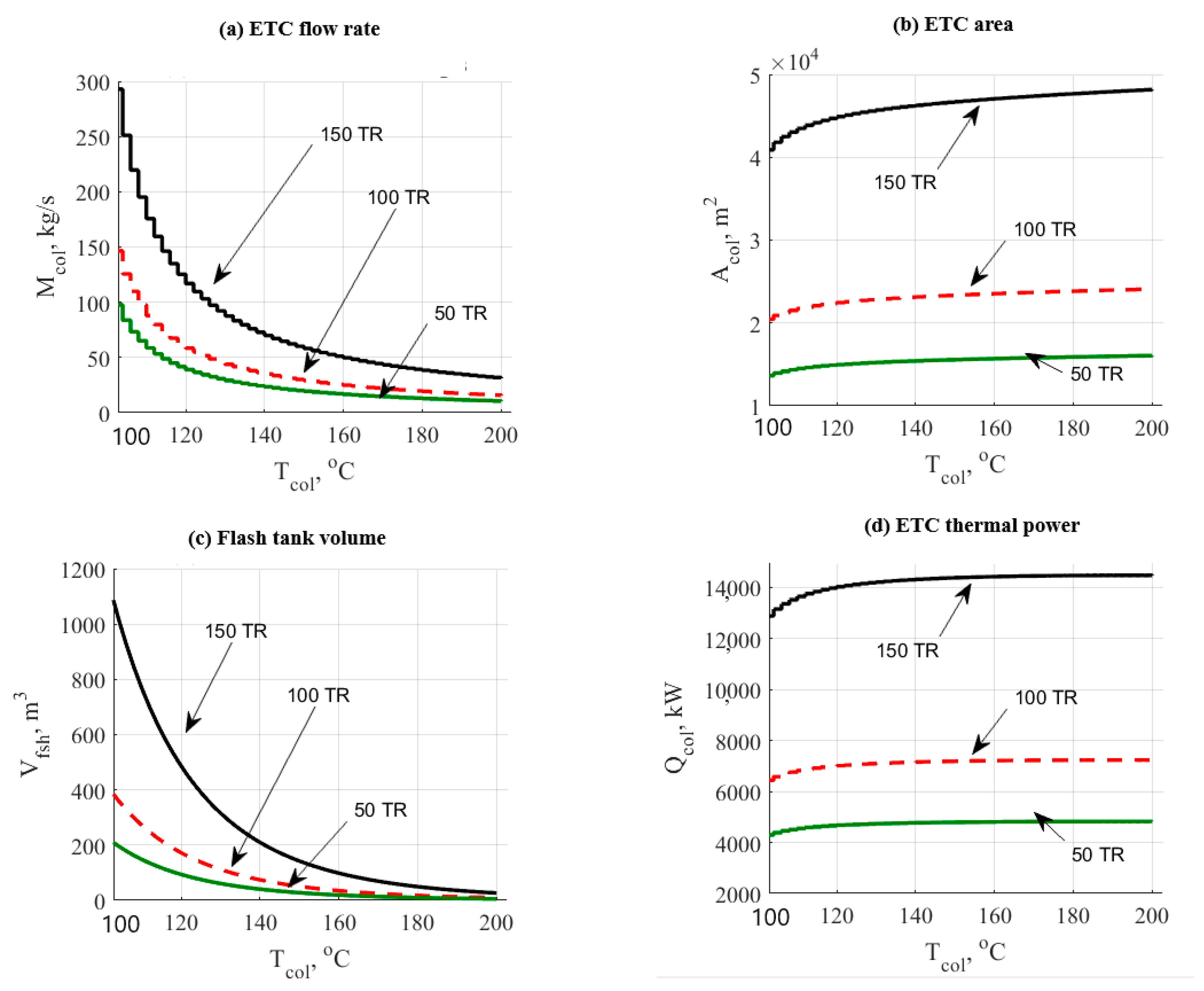
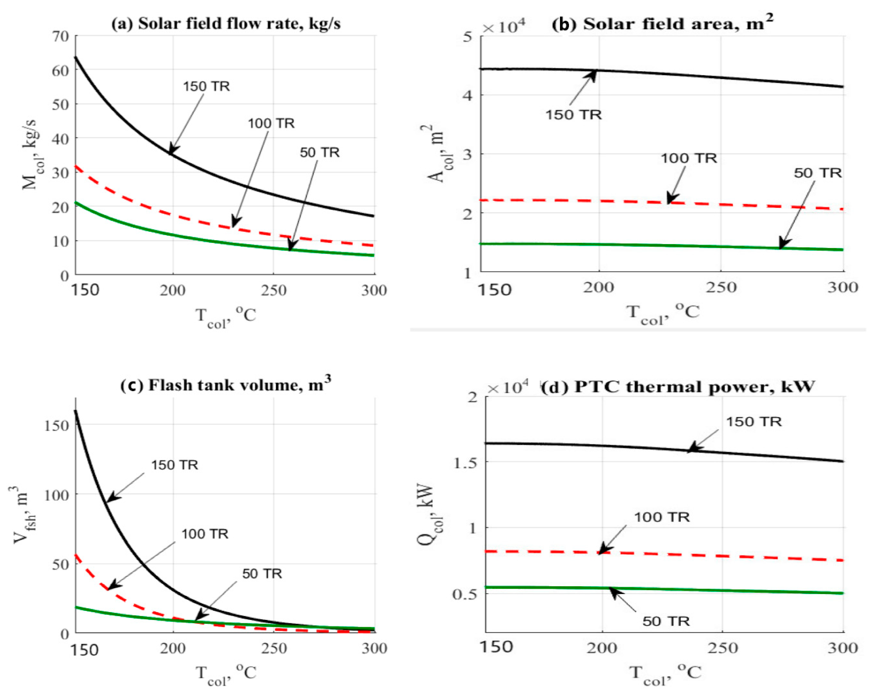
The simulation data delivers temperature data of solar field at various cooling loads (50–150TR), and at different solar collector working temperature values (100–200 °C for ETC and 200–300 °C for PTC). Figure 2 and Figure 3 depict the obtained results based on the influence of the temperature of the solar collector on the other design parameters, such as mass flow rates, and design aspects. Figure 2a and Figure 3a show the impact of the solar collector temperature on solar field mass flow rate. The mass flow rate shows a strong temperature dependency. Higher temperature of the solar collector also causes a large decline in the mass flow rate of the solar field. The primary cause for this effect was referring to the energy balance throughout the solar field as provided in this partnership $Q_{th}=M_{col}^{.}\times C_p\times \left(T_o-T_i\right)$.

Even so, in contrast with the ETC, the PTC yielded a lower average mass flow rate dependent on an increase in top temperature. The solar field area also has an increasing influence depending on the temperature rise. This effect is shown in Figure 2b and Figure 3b. The increase in the outlet temperature is quite certain to increase the area of the solar field. However, the PTC is registered less in the total area vs. the ETC. Figure 2c and Figure 3c represent a significant impact on flash tank volume by the increase in solar collector temperature. Even so, in comparison with the ETC, PTC showed low tank volume results.

The total solar thermal energy variations due to the change in the upper temperature of the solar field have been depicted in Figure 2d and Figure 3d. Raising the upper solar field temperature increases solar thermal power in the entire solar field in both cases. The exit temperature is an important value for designing the solar field. For ETC collectors and PTC solar collectors, a temperature level of 150~200 °C and 250~300 °C are suggested in this study. Based on the current obtained results, it is quite interesting to assign the operating temperature as follows:

• T_a = 35 °C.
• T_c = 43 °C.
• T_e = 7~10 °C.
• T_g = 85~90 °C.
• ETC T_high = 150~200 °C.
• PTC T_high = 250~300 °C.

5.1.2. Effect of Cooling Load

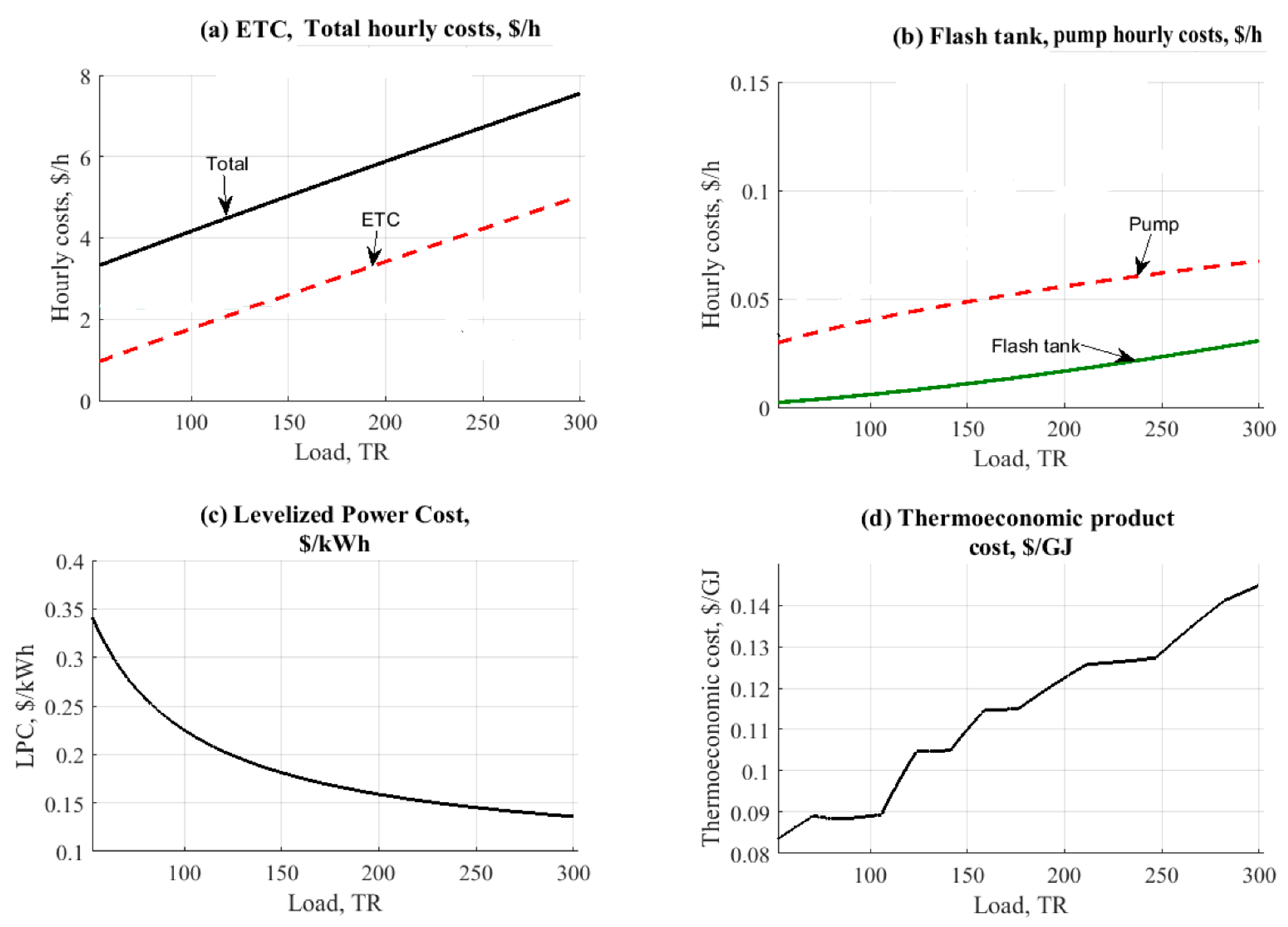
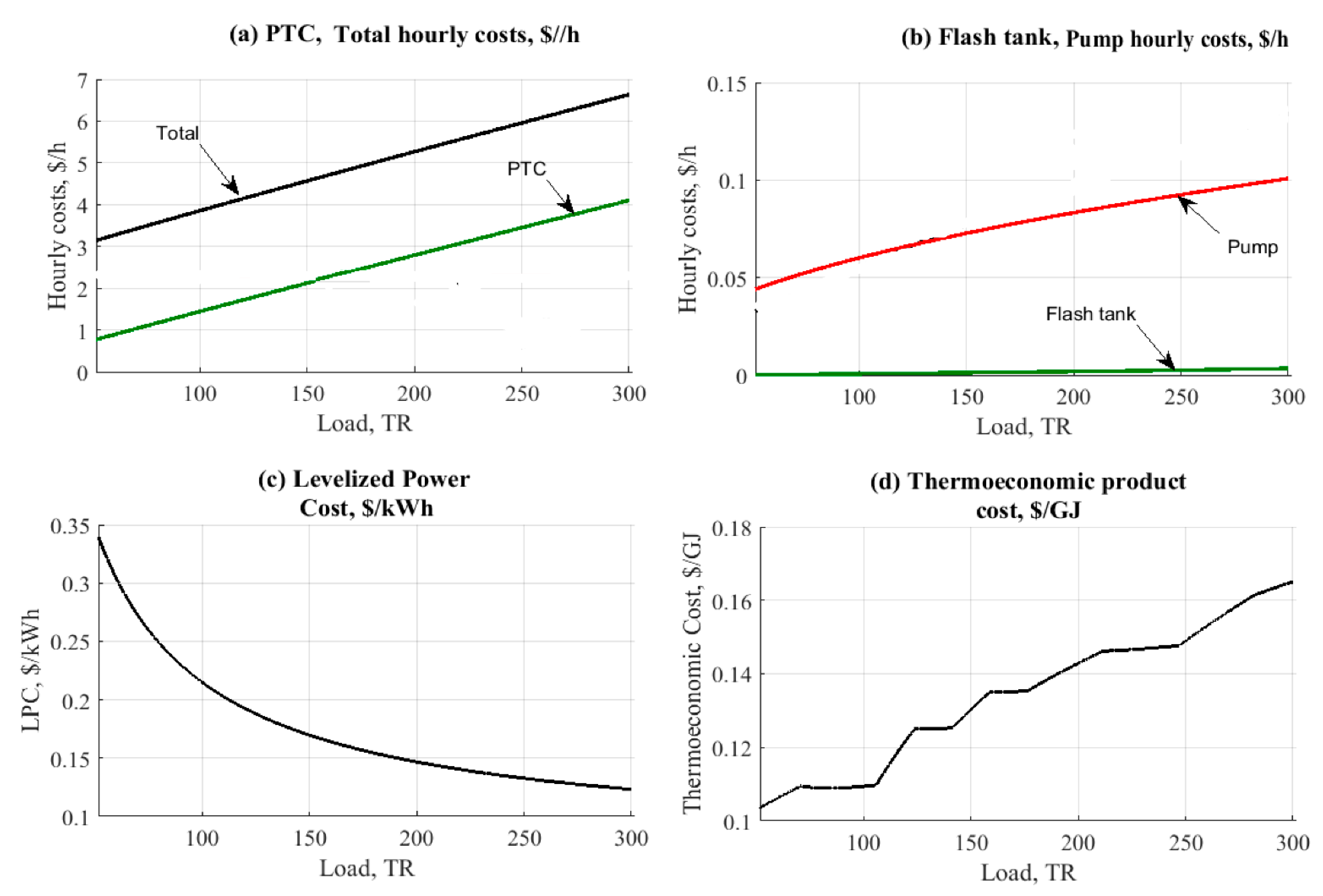
Figure 4 and Figure 5 demonstrate the influence of cooling load on cycles ETC/H₂O-LiBr and PTC/H₂O-LiBr. The two figures addressed the influence on the costs per hour, the cost of the levelized power, and the cost of the thermo-economic product. The thermo-economic parameter is very important because it reflect the combination between cost and exergy. At the same time, the exergy is also reflecting the maximum available work (gain) that be extracted from any system putting in consideration the entropy generation minimization. As expected, the trend in the figure has been increasing due to the load and energy consumption of all units. The solar collectors showed the largest hourly cost values compared to the corresponding other units, as illustrated in Figure 4a and Figure 5a.

Even so, the PTC is reported to be 12% lower than the ETC associated with the hourly cost variable. The key factor was the rise in the working temperature of the collector (250 °C vs. 150 °C). More steam is produced for the AAC cycle by raising the collector temperature. The influence of increasing cooling load on pumps and flashing tanks is illustrated in Figure 4b and Figure 5b. The figures clearly show that the pumps register slightly higher than the flash tank by the total work required.

Figure 4c and Figure 5c demonstrate the impact of cooling on the cost of levelized power, $/kWh. The outcomes are almost the same depending on the approximate results of the related pumping unit in both configurations. The leveled power cost varied from 0.15 $/kWh to 0.35 $/kWh. A similar close was observed when comparing the cost of the thermo-economic product. For both configurations, the outcomes have been centralized at 0.08 to 0.14~0.16 $/GJ with a minor advantage to the ETC (Figure 4d and Figure 5d). As expected, a higher load will increase the exergy cost. Both PTC and ETC have been identified as the main reason for such an effect due to the large area that is required for covering the load.

5.2. Ammonia-Water (NH₃-H₂O) Cycle Results

5.2.1. Effect of Top Solar Field Temperature (NH₃-H₂O)

The upper temperature of the solar field is considered a very significant factor within this cycle. Figure 6 and Figure 7 demonstrate the changes in the performance and design variables for both ETC and PTC installations. The temperature range for ETC was 110 °C up to 200 °C. For PTC, the temperature range was 150 °C up to 300 °C.

Figure 6a indicates the influence of the top ETC temperature on the mass flow rate of the solar field. The figure also shows that a rise in the upper temperature reduces the overall mass flow rate in the solar field as a common result of the energy balance. An identical trend was also observed in Figure 7a that depicts the PTC operation. Even so, the PTC granted smaller flow rates, leading to a lower cost. The difference is considerable when comparing 50 kg/s to 300 kg/s @150TR for the ETC and 15 kg/s to 65 kg/s @150TR for the PTC.

Figure 6b and Figure 7b display the influence of solar field temperature on the design area of the solar collectors. The variations on the two figures were not massive, even though the lowest area, i.e., the lowest cost and control is reported for the PTC as anticipated. Raising the temperature of PTC will reduce both the loops and unit numbers as well. The number of loop variables is influenced by the total area of the PTC needed for the load. For instance, the ETC at 150TR would consume around 45,000 m² to 50,000 m². However, the PTC in the same operating conditions will require approximately 45,000 m² down to 40,000 m².

For both situations, the volume of the flash tank has been depicted in Figure 6c and Figure 7c. The distinction is very obvious with the PTC advantage. Increasing the upper-temperature level of the solar field will reduce the volume of the flashing tank. However, the ETC would require bigger tanks due to a massively lower dryness fraction relative to the PTC process.

For ETC, Figure 6d represents the effect on the thermal power, kW; the rise in working temperature also enhances the solar thermal energy. Figure 7d demonstrates the influence on the thermal power of the PTC. The figure exhibits a descending behavior concerning the upper solar field temperature increase. In general, the increase in AAC unit load would require a larger solar field area, resulting in the mass flow rate increase.

Ranges of 150~200 °C and 250~300 °C are advocated for ETC and PTC solar thermal collectors in this paper. Depending on the latest data achieved, it is quite important to assign the working temperature as follows:

• T_a = 35 °C.
• T_c = 43 °C.
• T_e = 7~10 °C.
• T_g = 85~90 °C.
• ETC T_high = 150~200 °C.
• PTC T_high = 250~300 °C.

5.2.2. Effect of Cooling Load Effect (NH₃-H₂O)

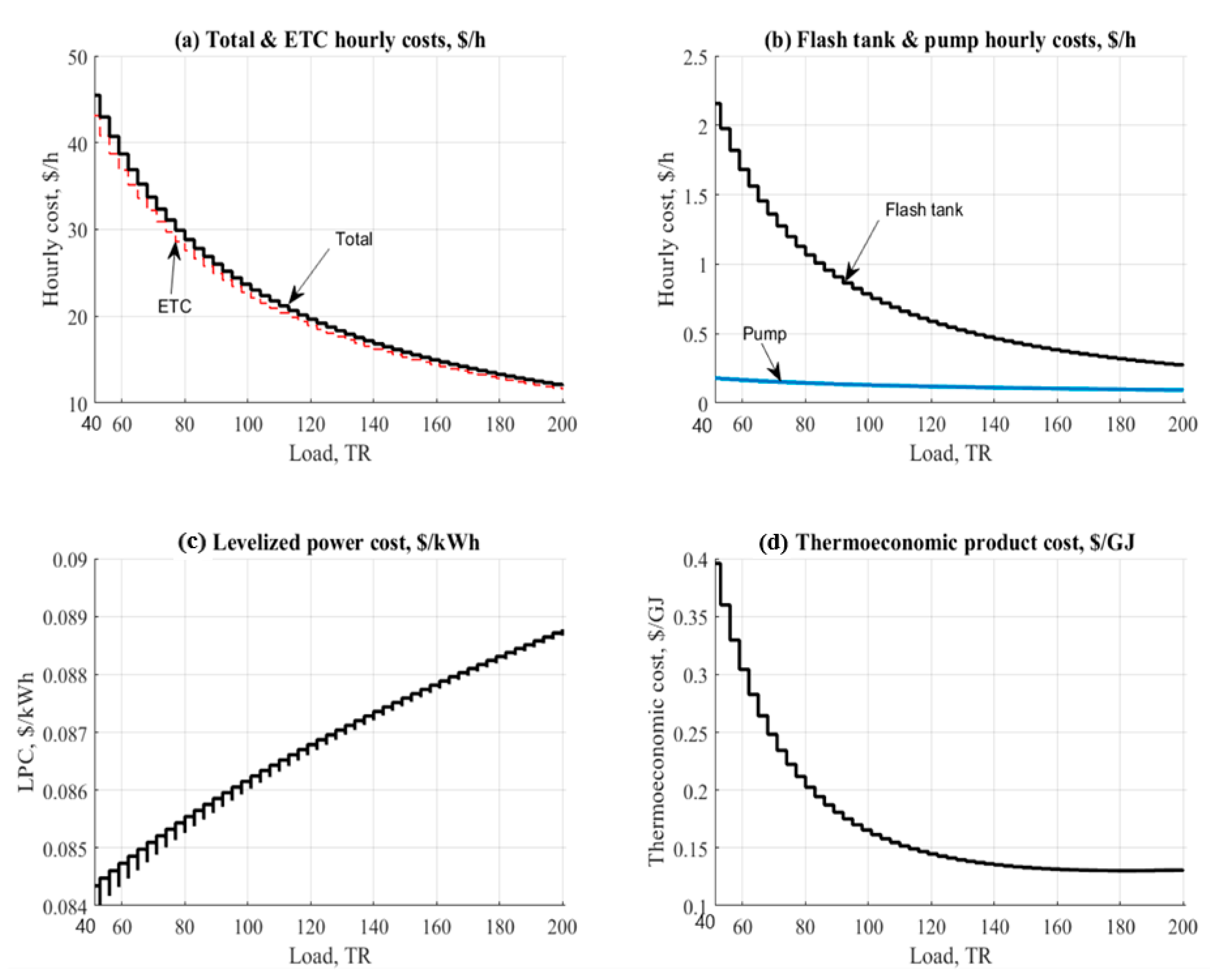
The effect of cooling capacity on the ETC-NH₃-H₂O and PTC-NH₃-H₂O configurations is illustrated in Figure 8 and Figure 9. The two figures cover the impact on the costs per hour, the cost of the leveled energy, and the cost of the thermo-economic product. The trend in the figure was, as predicted, in a variable mode owing to the energy load and required by all units. The solar collectors showed the largest hourly cost values among the other units as illustrated in Figure 8a and Figure 9a.

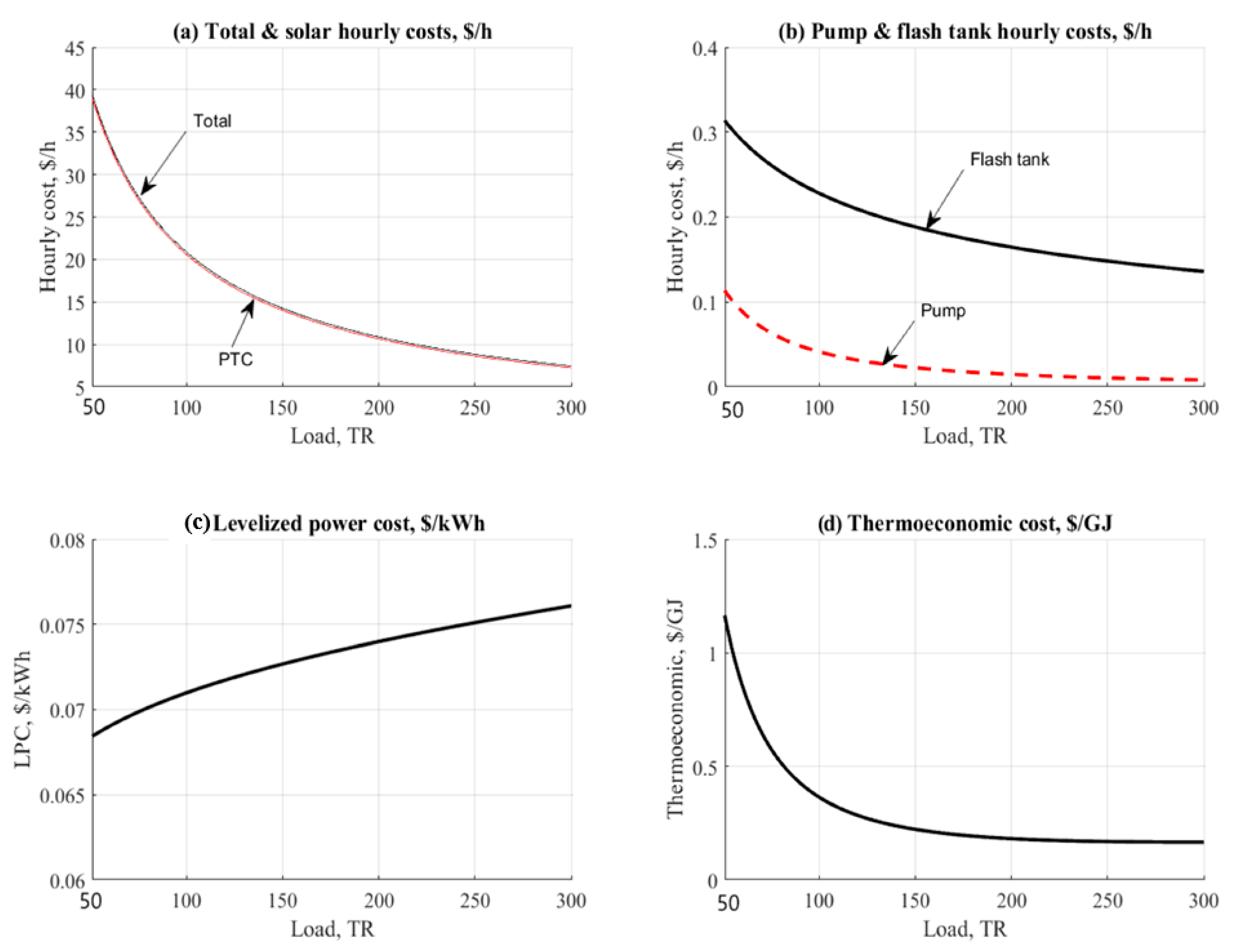
However, the PTC was lower by 8% against the ETC, associated with the variable cost of hour metric. This was mainly due to the increase in the collector’s working temperature (250 °C vs. 150 °C). The increase in the temperature of the collector would produce further steam for the AAC unit. Pumps and flashing tanks are seen in Figure 8b and Figure 9b. It is clear from the figures that the flashing tank is recorded higher than the pump unit based on the total tank volume. PTC operation was recorded lower in flashing tank hourly cost because it has lower tank volume 0.2–0.3 $/h vs. 0.5–2.2 $/h. Figure 8c and Figure 9c display the impact of cooling capacity on the cost of levelized power rate, $/kWh. The outcomes are almost the same depending on the approximate results of the related pumping unit in both configurations. The leveled power cost varied from 0.07 $/kWh to 0.08 $/kWh for PTC and ETC, respectively. Identical close behavior was observed when compared related to the cost of the thermo-economic product. The results ranged from $0.1 to $1/GJ in both configurations with a smaller advantage for the ETC (Figure 8d and Figure 9d).

5.3. Case Study Results

The case study introduced in this section compares all the configurations at a specified load point. This case study was conducted in a sports hall situated in Baghdad, Iraq. The stadium costs $14 million, and the 3000-seat capacity indoor sports facilities are focused on basketball, volleyball, and athletics. The entire project employs central air conditioning for an air-cooled absorption chiller of 700~800 kW. Its evaporator would be designed to operate in the range of 7~12 °C.

Table 2. Case study results @ 200 TR cooling load.

Solar Radiation, W/m2	500
Tamb, °C	25
Ta, Te, Tg, Tc, Tcol, °C	=30, 10, 90, 40, 175	=30, 10, 90, 40, 175	=30, 10, 90, 40, 250	=30, 10, 90, 40, 250
Load, TR	200
Target cooled air, °C	20
Interest rate, %	5
Load factor, %	95
Plant life time, yr	20
Electric cost, $/kWh	0.065
Pumps efficiency, %	75
Configuration:	ETC-H2O/LiBr	ETC-NH3/H2O	PTC-LiBr/H2O	PTC-NH3/H2O
Solar field:
Total solar field area, m2	3022	11,880	2433	11,020
Solar thermal power, kW	918.6	3612	890	4051
Inlet temperature, °C	91.64	91.82	92.66	92.04
Mass flow rate, kg/s	2.582	10.17	1.327	8.727
Inlet exergy, kW	1436	5646	1136	4217
Exergy destruction, kW	1191	4683	930	5143
Flash tank:
Height/Width, m	1.742/0.852	3.381/1.655	0.837/0.41	2.743/1.343
Volume, m3	0.9942~1	7.276	0.1106	3.883
Total flow rate, kg/s	2.582	10.17	1.327	8.727
Water content, kg/s	2.1	8.551	0.897	6.91
Dryness fraction	0.1667	0.1595	0.324	0.208
Exergy destruction, kW	134.3	391.1	180.8	515.6
AAC unit:
Qa, kW	743.3	1251	743.3	1153
Aa, m2	190.5	23.37	190.5	21.3
Mstr, kg/s	1.391	1.428	1.391	1.428
Mwk, kg/s	1.092	0.778	1.092	0.778
Xa-hex	0.4893	--	0.4893	--
Xhex-NH3	--	0.4554	--	0.4554
Ahex, m2	1.313	7.837	1.313	6.73
Qg, kW	787.8	1407	787.8	1256
Ag, m2	4.299	5.123	4.299	4.574
Driving steam flow, kg/s	0.4034	2.07	0.4034	1.848
Xg-hex	0.6233	--	0.6233	--
Qc, kW	747.8	694.9	747.8	694.9
Ac, m2	37.45	9.1	37.45	9.1
Mr, kg/s	0.299	0.6505	0.299	0.6505
Qe, kW	703.4	703.4	703.4	703.4
Ae, m2	36.35	41.15	36.35	41.15
FHP, kW	29.33~30	70.64	29.33~30	70.64
Mair, kg/s	68	119.5~120	68	119.5~120
COP/COPmax	0.89/1.56	0.5/1.559	0.89/1.56	0.5/1.559
RPR	0.573	0.3206	0.573	0.3591
Exergy destruction, kW	729.9	1010	729.9	977.3
Pump unit:
Wp, kW	3.204	12.63	7.338	18.97~19
Exergy destruction, kW	14.8	64.7	12.33	62.25
Cost & Thermo-economics:
Zcol, $/h	3.918	11.75	2.604	10.93
Zfsh, $/h	0.02	0.11	0.001	0.06
Zaac, $/h	0.121	0.0487	0.121	0.04716
Zp+f, $/h	0.055	0.256	0.1743	0.2652
Ztot, $/h	4.114	12.16	2.9	11.3
LPC, $/kWh	0.165	0.089	0.1557	0.0744
cp, $/GJ	0.1474	0.144	0.1602	0.1554

reports the results data in the case of using the solar absorption cooling cycle for all installations. A cooling load of 200TR was chosen for comparison. The ambient working conditions are set to a specified amount for simplicity. Regarding the results of the solar field, the PTC/H₂O-LiBr configuration proved to be the lowest in the required area, which is quite significant for decreasing the required area. The ETC/H₂O-LiBr was the next one. The same behavior was observed in PTC/NH₃-H₂O vs. ETC/NH₃-H₂O configurations. With respect to design features that include the design of the flash tank, the operation of the PTC/H₂O-LiBr configuration provided the lowest results, and this was very advantageous by 0.11 m³, while the ETC/H₂O-LiBr has 1 m³ and the PTC/NH₃-H₂O had 3.8 m³. We also observed the same trend concerning the exergy destruction and dryness fraction. Exergy destruction analysis showed that the most critical part in the system that causes the highest percent of the exergy destruction is the solar collectors due to the big difference between the highest exergy input, as it depends on the sun temperature, and the exergy output due to the heat transfer to the heat carrier fluid (water). Consequently, in order to decrease the solar collector’s exergy loss, the heat transfer between the solar radiation and the heat carried fluid has to be enhanced through new designs and investigations. For the entire AAC, the highest exergy loss was experienced in the absorber and generator. Therefore, special attention must be considered in the design of these components. The AAC was found to be lower in design results based on the H₂O-LiBr operation. The results expose that PTC is regarded as a cycling advantage for ETC operation. The idle driving steam has been reported by PTC/H₂O-LiBr with 0.4 kg/s, which led to a reduced volume of the flashing tank and solar field area. The COP value was substantial relative to the H₂O-LiBr cycle. For cost per hour, PTC/H₂O-LiBr was noticed to be the lowest among the others. By reaching 5.2 $/hr, PTC/H₂O-LiBr was identified as the best alternative for this case study. The lowest hourly costs for the solar array were regarded as the vital term to judge the cost of the system. The thermo-economic cost was almost the same for all configurations in the range of 0.14–0.16 $/GJ with an advantage for H₂O-LiBr configuration.

6. Conclusions

This study introduced different configurations of solar-assisted absorption air conditions (AAC) cycles. The proposed system is powered by solar energy. The system configuration combines solar field (PTC/ETC), flashing tank, and absorption chiller (H₂O-LiBr/NH₃-H₂O). A case study of 200 TR cooling is applied to the simulation program. Energetic and exegetic results are presented and have revealed that:

• Design aspects such as solar area and flashing tank volume were found have a great influence on the cycle cost.
• Among all configurations, PTC-H₂O-LiBr gives a remarkable result comparing against the ETC.
• For case study, PTC-H₂O-LiBr was recorded the best based on design and hourly costs. The required solar area was in the range of 2000~2500 m². Meanwhile, the total hourly cost was in the range of 4~5 $/h, which is quite attractive.
• Absorption chiller coefficient of performance was in the range of 0.5 to 0.9.
• The total rate of exergy destruction of the AAC was in the range of 55 kW.
• Solar field harvests a larger amount of exergy destruction rates for all configurations due to the large area and mass flow rate effect. PTC-H₂O-LiBr resulted in a 930~1000 kW of exergy destruction rate comparing against PTC-NH₃-H₂O, which resulted a value of 4600~5000 kW.
• PTC-H₂O-LiBr gives the lowest values related to exergy destruction rates for all units.
• PTC-H₂O-LiBr gives the lowest value of flashing tank design aspects such as width 0.4~0.5 m, height 0.8 m, and volume 0.11 m³. ETC-H₂O-LiBr comes next with a total flashing tank equal to ~1 m³.
• The thermo-economic cost is almost the same for all configurations in the range of 0.14–0.16 $/GJ with an advantage for H₂O-LiBr configuration.
• It is quite clear that PTC-H₂O-LiBr followed by ETC-H₂O-LiBr have remarkable results according to the terms of energy, design, and cost. Generally, PTC system is considered the best choice for H₂O-LiBr or NH₃-H₂O.

References

- Wang, R.Z.; Wu, J.Y.; Dai, Y.J.; Wang, W.; Jiangzhou, S. Adsorption Refrigeration; China Mechanical Industry Press: Beijing, China, 2002. [Google Scholar]
- IEA. Global CO2 Emissions in 2019; IEA: Paris, France, 2020; Available online: https://www.iea.org/articles/global-co2-emissions-in-2019 (accessed on 10 September 2020).
- Al-Alili, A.; Hwang, Y.; Radermacher, R. Review of solar thermal air conditioning technologies. Int. J. Refrig. 2014, 39, 4–22. [Google Scholar] [CrossRef]
- Mone, C.D.; Chau, D.S.; Phelan, P.E. Economic feasibility of combined heat and power and absorption refrigeration with commercially available gas turbines. Energy Convers. Manag. 2001, 42, 1559–1573. [Google Scholar] [CrossRef]
- Rodríguez-Muñoz, J.L.; Belman-Flores, J.M. Review of diffusion–absorption refrigeration technologies. Renew. Sustain. Energy Rev. 2014, 30, 145–153. [Google Scholar] [CrossRef]
- Bataineh, K.; Taamneh, Y. Review and recent improvements of solar sorption cooling systems. Energy Build. 2016, 128, 22–37. [Google Scholar] [CrossRef]
- Syed, A.; Maidment, G.G.; Tozer, R.M.; Missenden, J.F. A Study of the Economic Perspectives of Solar Cooling Schemes. In Proceedings of the CIBSE National Conference, Part 2, London, UK, 14 October 2002. [Google Scholar]
- Balaras, C.A.; Hans-Martin, H.; Wiemken, E.; Grossman, G. Solar cooling: An overview of European applications design guidelines. ASHRAE J. 2006, 48, 14. [Google Scholar]
- Li, M.; Xu, C.; Hassanien, R.H.E.; Xu, Y.; Zhuang, B. Experimental investigation on the performance of a solar powered lithium bromide–water absorption cooling system. Int. J. Refrig. 2016, 71, 46–59. [Google Scholar] [CrossRef]
- Mazloumi, M.; Naghashzadegan, M.; Javaherdeh, K.J.E.C. Simulation of solar lithium bromide–water absorption cooling system with parabolic trough collector. Energy Convers. Manag. 2008, 49, 2820–2832. [Google Scholar] [CrossRef]
- Shirazi, A.; Taylor, R.A.; White, S.D.; Morrison, G.L. Multi-effect absorption chillers powered by the sun: Reality or reverie. Energy Procedia 2016, 91, 844–856. [Google Scholar] [CrossRef] [Green Version]
- Zacarías, A.; Venegas, M.; Lecuona, A.; Ventas, R.; Carvajal, I. Experimental assessment of vapour adiabatic absorption into solution droplets using a full cone nozzle. Exp. Therm. Fluid Sci. 2015, 68, 228–238. [Google Scholar] [CrossRef]
- Rajasekar, D.; Ponshanmugakumar, A.; Rajavel, R. Design and Performance Validation of Vapour Absorption Solar Air Conditioning System. Int. J. Future Revolut. Comput. Sci. Commun. Eng. 2017, 3, 115–119. [Google Scholar]
- Flores, V.H.F.; Román, J.C.; Alpírez, G.M. Performance analysis of different working fluids for an absorption refrigeration cycle. Am. J. Environ. Eng. 2014, 4, 1–10. [Google Scholar]
- Gebreslassie, B.H.; Medrano, M.; Boer, D. Exergy analysis of multi-effect water–LiBr absorption systems: From half to triple effect. Renew. Energy 2010, 35, 1773–1782. [Google Scholar] [CrossRef]
- Kilic, M.; Kaynakli, O. Second law-based thermodynamic analysis of water-lithium bromide absorption refrigeration system. Energy 2007, 32, 1505–1512. [Google Scholar] [CrossRef]
- Karakas, A.; Egrican, N.; Uygur, S. Second-law analysis of solar absorption-cooling cycles using lithium bromide/water and ammonia/water as working fluids. Appl. Energy 1990, 37, 169–187. [Google Scholar] [CrossRef]
- Dincer, I.; Ratlamwala, T.A.H. Fundamentals of Absorption Refrigeration Systems. In Integrated Absorption Refrigeration Systems; Springer: Cham, Switzerland, 2016; pp. 1–25. [Google Scholar]
- Lu, Z.S.; Wang, R.Z. Experimental performance investigation of small solar air-conditioning systems with different kinds of collectors and chillers. Solar Energy 2014, 110, 7–14. [Google Scholar] [CrossRef]
- Colorado, D.; Rivera, W. Performance comparison between a conventional vapor compression and compression-absorption single-stage and double-stage systems used for refrigeration. Appl. Therm. Eng. 2015, 87, 273–285. [Google Scholar] [CrossRef]
- Wang, Y.; Wang, C.; Feng, X. Optimal match between heat source and absorption refrigeration. Comput. Chem. Eng. 2017, 102, 268–277. [Google Scholar] [CrossRef]
- Du, S.; Wang, R.Z.; Chen, X. Development and experimental study of an ammonia water absorption refrigeration prototype driven by diesel engine exhaust heat. Energy 2017, 130, 420–432. [Google Scholar] [CrossRef]
- Al-Falahi, A.; Alobaid, F.; Epple, B. Design and Thermo-economic Comparisons of Large Scale Solar Absorption Air Conditioning Cycles. Case Stud. Therm. Eng. 2020, 22, 100763. [Google Scholar] [CrossRef]
- Al-Falahi, A.; Alobaid, F.; Epple, B. Thermo-Economic Evaluation of Aqua-Ammonia Solar Absorption Air Conditioning System Integrated with Various Collector Types. Entropy 2020, 22, 1165. [Google Scholar] [CrossRef] [PubMed]
- NIST Chemistry WebBook, SRD 69. Available online: https://webbook.nist.gov/chemistry/name-ser/ (accessed on 3 October 2020).
- Vakiloroaya, V.; Ha, Q.; Skibniewski, M.J. Modeling and experimental validation of a solar-assisted direct expansion air conditioning system. Energy Build. 2013, 66, 524–536. [Google Scholar] [CrossRef] [Green Version]
- Carles Bruno, J.; López-Villada, J.; Letelier, E.; Romera, S.; Coronas, A. Modelling and Optimisation of Solar Organic Rankine Cycle Engines for Reverse Osmosis Desalination. Appl. Therm. Eng. 2008, 28, 2212–2226. [Google Scholar] [CrossRef]
- Nafey, A.S.; Sharaf, M.A.; García-Rodríguez, L. A New Visual Library for Design and Simulation of Solar Desalination Systems (SDS). Desalination 2010, 259, 197–207. [Google Scholar] [CrossRef]
- Eldean, M.A.S.; Soliman, A.M. A new visual library for modeling and simulation of renewable energy desalination systems (REDS). Desalin. Water Treat. 2013, 51, 6905–6920. [Google Scholar] [CrossRef]
- Singh, R.; Kumar, D.R. Theoritical Analysis of Nh3-H2o Refrigeration System Coupled with Diesel Engine: A Thermodynamic Study. IOSR J. Mech. Civ. Eng. 2014, 11, 29–36. [Google Scholar] [CrossRef]
- Li, K.W. Applied Thermodynamics: Availability Method and Energy Conversion; CRC Press: Boca Raton, FL, USA, 1995. [Google Scholar]
- Bejan, A.; Tsatsaronis, G.; Moran, M.J. Thermal Design and Optimization; Wiley: New York, NY, USA, 1996; Chapter 8. [Google Scholar]
- Sharaf, M.A.; Nafey, A.S.; García-Rodríguez, L. Author’s Personal Copy Thermo-Economic Analysis of Solar Thermal Power Cycles Assisted MED-VC (Multi Effect Distillation-Vapor Compression) Desalination Processes. Energy 2011, 36, 2753–2764. [Google Scholar] [CrossRef]
- Sharaf, M.; Nafey, A.; Desalination, L.G.-R. Exergy and Thermo-Economic Analyses of a Combined Solar Organic Cycle with Multi Effect Distillation (MED) Desalination Process. Desalination 2011, 272, 135–147. [Google Scholar] [CrossRef]
- Castro, M.M.; Song, T.W.; Pinto, J.M. Minimization of operational costs in cooling water systems. Chem. Eng. Res. Des. 2000, 78, 192–201. [Google Scholar] [CrossRef]
Figure 1.
Absorption air-conditioning system integrated with solar thermal collector. (a) Parabolic trough collector PTC; (b) Evacuated tube collector ETC [24].
Figure 2.
Data results for ETC/H2O-LiBr cycle vs. variation in exit upper temperature of the solar field. (a) Collector flow rate. (b) Solar collector area. (c) Flash tank volume. (d) Solar thermal power.
Figure 3.
Data results for PTC/H2O-LiBr cycle vs. variation in exit upper temperature of the solar field. (a) Collector flow rate. (b) Solar collector area. (c) Flash tank volume. (d) Solar thermal power.
Figure 4.
Data results for ETC-H2O-LiBr cycle vs. change in cooling load. (a) ETC total hourly cost. (b) Flash tank and pump hourly cost. (c) Levelized power cost. (d) Thermo-economic product.
Figure 5.
Data results for PTC-H2O-LiBr cycle vs. change in cooling load. (a) PTC total hourly cost. (b) Flash tank and pump hourly cost. (c) Levelized power cost. (d) Thermo-economic product.
Figure 6.
Data results for ETC/NH3- H2O cycle vs. variation in upper temperature of the solar field. (a) Collector flow rate. (b) Solar collector area. (c) Flash tank volume. (d) Solar thermal power.
Figure 7.
Data results for PTC/NH3- H2O cycle vs. variation in upper temperature of the solar field. (a) Collector flow rate. (b) Solar collector area. (c) Flash tank volume. (d) Solar thermal power.
Figure 8.
Data results for ETC/NH3-H2Ocycle vs. cooling load. (a) ETC total hourly cost. (b) Flash tank and pump hourly cost. (c) Levelized power cost. (d) Thermo-economic product.
Figure 9.
Data results for PTC/NH3-H2O cycle vs. cooling load. (a) PTC total hourly cost. (b) Flash tank and pump hourly cost. (c) Levelized power cost. (d) Thermo-economic product.