
Non-Deterministic Methods and Surrogates in the Design of Rockfill Dams

Département de Génie Mécanique, École de Technologie Supérieure, Montréal, QC H3C 1K3, Canada
*
Author to whom correspondence should be addressed.
Appl. Sci. 2021, 11(8), 3699; https://0-doi-org.brum.beds.ac.uk/10.3390/app11083699
Submission received: 23 March 2021
/
Revised: 14 April 2021
/
Accepted: 16 April 2021
/
Published: 20 April 2021
(This article belongs to the Section Civil Engineering)
Abstract
:The parameters of the constitutive models used in the design of rockfill dams are associated with a high degree of uncertainty. This occurs because rockfill dams are comprised of numerous zones, each with different soil materials, and it is not feasible to extract materials from such structures to accurately ascertain their behavior or their respective parameters. The general approach involves laboratory tests using small material samples or empirical data from the literature. However, such measures lack an accurate representation of the actual scenario, resulting in uncertainties. This limits the suitability of the model in the design process. Inverse analysis provides an option to better understand dam behavior. This procedure involves the use of real monitored data, such as deformations and stresses, from the dam structure via installed instruments. Fundamentally, it is a non-destructive approach that considers optimization methods and actual performance data to determine the values of the parameters by minimizing the differences between simulated and observed results. This paper considers data from an actual rockfill dam and proposes a surrogate assisted non-deterministic framework for its inverse analysis. A suitable error/objective function that measures the differences between the actual and simulated displacement values is defined first. Non-deterministic algorithms are used as the optimization technique, as they can avoid local optima and are more robust when compared to the conventional deterministic methods. Three such approaches, the genetic algorithm, differential evolution, and particle swarm optimization are evaluated to identify the best strategy in solving problems of this nature. A surrogate model in the form of a polynomial regression is studied and recommended in place of the actual numerical model of the dam to reduce computation cost. Finally, this paper presents the relevant dam parameters estimated by the analysis and provides insights into the performance of the three procedures to solve the inverse problem.
1. Introduction
The design of Rockfill dams presents significant challenges to geotechnical engineers because of the uncertainties and the complex structural and material characteristics involved [1]. Computational methods have played an important role in addressing the associated difficulties. These methods have been successful in providing better dam designs that are more reliable and have helped in reducing the cost and time of dam construction. Such approaches usually involve the development of numerical models, and the application of the finite element method (FEM) in this discipline has become the norm. This successful use of the FEM could be attributed to its ability to provide a high degree of accuracy and to effectively deal with complex geometries and boundary conditions as well as material (rock/soil) nonlinearities [2,3]. However, the formulation of numerical models involves the approximation and simplification of the physical problem. In addition, the lack of information pertaining to material properties, external factors such as weather, and shortcomings in the applied constitutive law limits such models in the precise representation of actual dam behavior. In such a scenario, inverse analysis procedures can help to estimate associated parameters that are reliable and thereby improve the design of the dam under consideration.
Inverse analysis in essence is an optimization process. The approach involves two major components: an optimization algorithm that attempts to minimize an error/objective function, and a numerical model/solver. Instrumentation data, which may include the deformations, stresses, seepage, and other performance measurements of a dam, are used to define the error function. The optimization algorithm, together with the numerical solver, searches for optimum parameter values in order to minimize the objective function. Earlier, methods such as the conjugate gradient, steepest descent, and trust region were commonly used for these problems as optimization/search approaches [4]. However, soil and rocks present highly nonlinear behavior, and such methods are not always adequate to deal with them. Those methods may lead to the solution being trapped in local optima, or even fail to converge. To avoid such scenarios, non-deterministic techniques, also known as stochastic methods, are preferred [5].
Non-deterministic approaches are robust in nature and can avoid the pitfalls of non-convergence and local optima. The advent of powerful computer hardware and sophisticated software have mitigated several of the bottlenecks associated with non-deterministic methods, and they now find widespread use. A major drawback of using such an algorithm in an inverse analysis is the large number of function evaluations required, as this causes multiple calls to the FEM-based numerical solver, which significantly increases the computational cost. An ingenious approach to address this issue involves the use of regression models also known as Surrogate models, which are used as a “lookup table” in place of the actual numerical model.
This paper performs an inverse analysis for the real-world scenario of the Romaine-2 rockfill dam (recently constructed in the province of Quebec, Canada) [6]. Five soil parameters: shear modulus (G), Poisson coefficient (ν), friction angle (φ), cohesion (c), and specific weight (γ), are identified using the displacement values recorded near the core of the dam (from a vertical inclinometer). An appropriate error function between the measured and simulated values is prescribed to calculate these five parameters. A framework involving a surrogate-assisted non-deterministic approach for the optimization/search segment coupled with the commercially available PLAXIS package as the solver is proposed [7]. The surrogate-aided non-deterministic strategy is implemented using open-source tools such as Python, OpenTURNS [8], Scikit-learn, Pandas, NumPy, and Matplotlib. In the scientific community, there are numerous variants of non-deterministic approaches. However, the performance of such algorithms is problem-dependent, and they may even provide unsatisfactory results. This work analyzes three non-deterministic techniques—the genetic algorithm, particle swarm optimization, and differential evolution—in the context of an inverse analysis for rockfill dams. The efficiency and effectiveness of the three methods in solving inverse problems are compared and the most suitable algorithm is identified. A detailed description of the procedure involving the use of polynomial regression is also provided, along with the advantages of building a surrogate model. Finally, the estimated soil parameters for a specific zone of the Romaine-2 dam is presented.
2. Problem Description
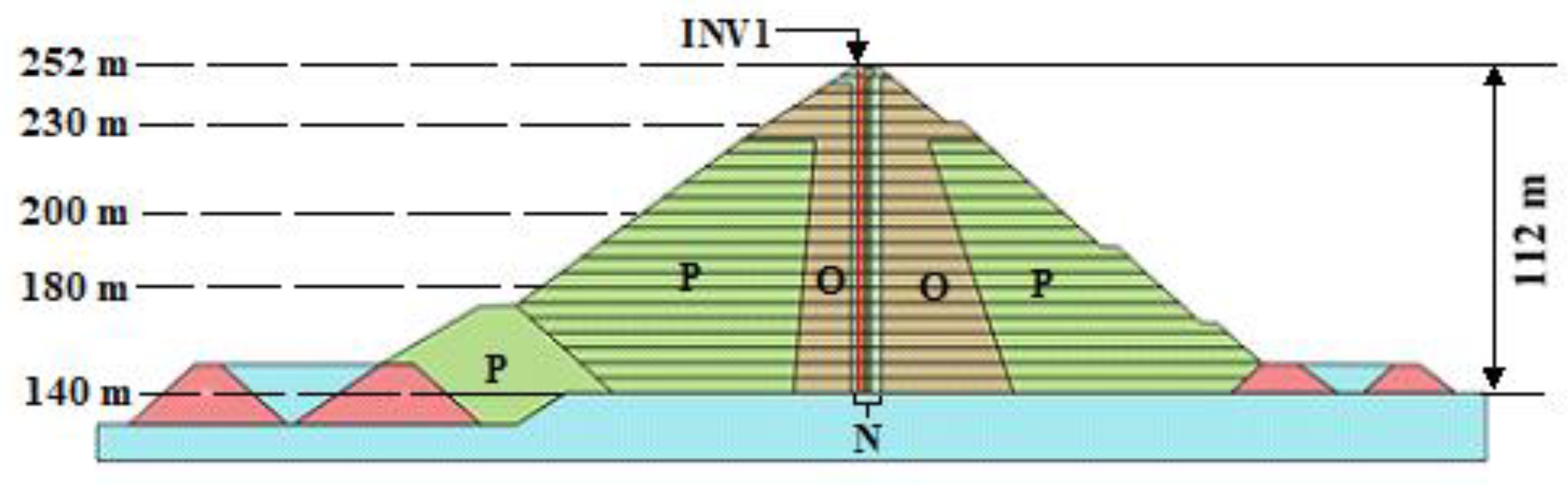
Figure 1 depicts a two-dimensional cross section of the Romaine-2 dam using Plaxis. The height of the dam is 112 m, and it has an asphalt core with a grouted rock foundation. Crushed stones that act as supports with a maximum size of 80 mm surround the core. Next to the support region lies the transition zone (N) composed of crushed stones that have a maximum size of 200 m. The internal shell zone (O) is comprised of particles with a maximum size of 0.6 m, and the external shell zone (P) is made of materials that reach a size of 1.2 m [6]. This investigation only considers the variations that occur in zone P, the section that covers the maximum portion of the Romaine-2 dam. Data from the vertical inclinometer INV01 located upstream (4.6 m to the left of the central axis) was used to construct the error function. The INV01 measurements used in this study represent the displacements during construction without the impoundment effects.
Constitutive laws relate external factors to the responses of a rockfill material governed by its internal constitution. Fundamentally, they describe the stress–strain characteristics of the soil. Mohr-Coulomb, Duncan-Chang, and Hardening soil are some of the main constitutive models applied in rockfill scenarios. The Mohr-Coulomb approach in general considers seven soil properties, whereas the Duncan-Chang and Hardening soil models involve 10 and 12 parameters, respectively. Numerous studies indicate that the Hardening soil method can accurately represent a wider set of geotechnical problems compared to the other two [9]. However, this study considers the Mohr-Coulomb approach because of its small number of required parameters. Nonetheless, it is possible to achieve a satisfactory level of accuracy with the Mohr-Coulomb with which to model the present scenario, and thus avoid the use of more complex methods [10].
The differences between the measured displacement values and those predicted by the numerical model in Plaxis are considered as errors. A simple error/objective function that incorporates this idea could be defined using the least squares method, and in the matrix form it is given by
where xmeas is a measured vector composed of measurements performed at different locations of the dam, and xcalc is a calculated vector that contains simulated displacement values at locations identical to those of the measured ones. An alternate generalized version of the above equation that considers an additional weighted term is given by
Various strategies could be applied to define the weighted term W (diagonal matrix) in Equation (2), depending upon the type of error. The effects due to a fault in the instrument or because of human factors, such as an error introduced by the procedure applied for extracting measurements, are two examples of error types. These aspects could be included in the function through W. In order to estimate such discrepancies between the measured and the simulated values, the maximum likelihood approach is a preferred choice [11]. The following equation describes the maximum likelihood method, which has a structure similar to that of Equation (2).
Cx is usually referred to as the covariance matrix, where the error structure of the instrument, or any prior information pertaining to the measurements, is plugged into the error/objective function. As observed in Figure 2, the measured plot indicates a significant amount of fluctuations, leading to a zigzag pattern. These fluctuations could be attributed to numerous factors that affect the inclinometers, including external temperature, calibration issues, and the manner in which they are handled and installed. To reduce the oscillations and obtain a smoother measurement curve, this work defines Cx in Equation (3) as:
where .
In the above equation, xmeasMean is the mean of the measured value, xmeasActual is the value recorded at a specific location by the inclinometer, and represents the standard deviation observed in the measured values. K is an integer constant in the range 1–3.
3. Review of Evolutionary and Population-Based Methods
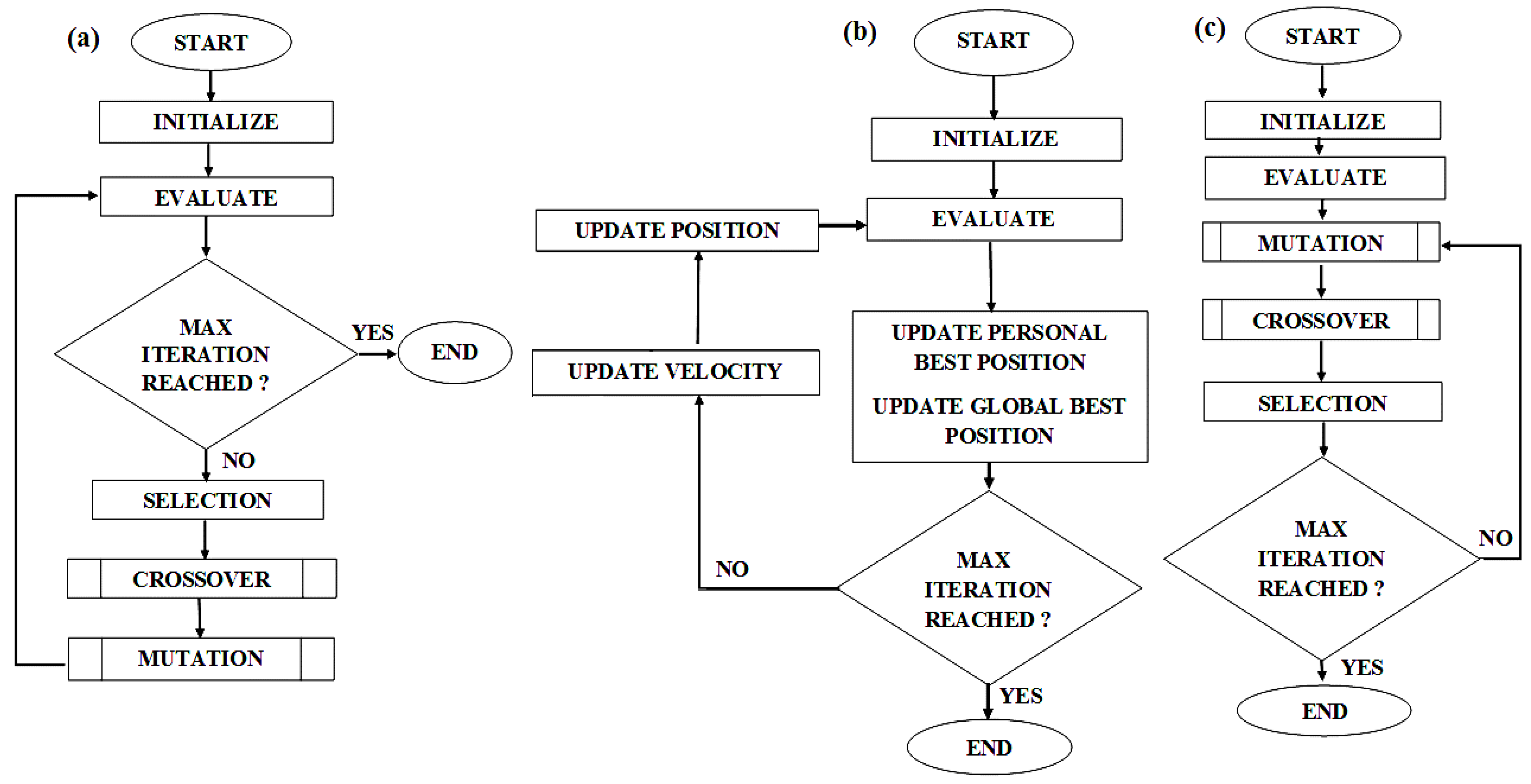
Traditional deterministic algorithms such as the quasi-Newton methods [4] are favored when a function is differentiable and convex. This ensures rapid convergence towards the optimum (minimum) solution. However, in many real-world engineering problems, there is no prior information about the overall system behavior. In addition, the requirement of gradient computation, and in some cases the need for a Hessian matrix, further complicates the application of such approaches. In the event when an objective function lacks continuity, the algorithms may even fail to converge. Under such circumstances, evolutionary and population-based strategies, also known as non-deterministic methods, are a preferred choice because the requirement of continuity in the objective function is not essential. Evolutionary/population-based methods are zeroth order techniques that use function values to perform their estimates. They offer additional benefits, including the ability to overcome local minima and seek a global optimum, the ability to deal with multiple objective functions, and their treatment of constraints is simple. The approach applied by non-deterministic methods involves the automatic discovery of regularities or unique features in the search space. These discoveries are further exploited in the form of a decomposition of the problem through the combination of pieces of the promising solutions found and by slightly perturbing these solutions. A downside to these algorithms is the high number of function evaluations associated with them. The following discussions highlight three non-deterministic strategies used in this work to perform the inverse analysis. Figure 3 presents the steps involved in the three algorithms.
3.1. Genetic Algorithm
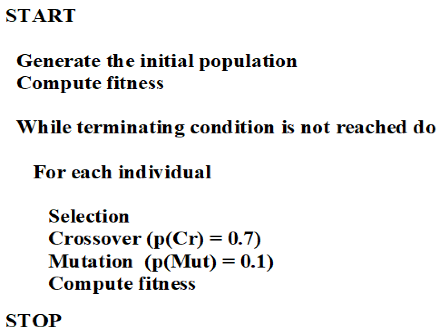
Genetic algorithm (GA) is an adaptive heuristic search algorithm first proposed by John Holland [12]. The GA mimics Darwinian evolution [13]. As in the natural selection of the evolution process, a GA simulates the survival of the fittest phenomenon, where the fittest individuals are selected to produce offspring for the next generation. A GA presents a robust mechanism that exploits a random search to solve optimization problems. The fundamental steps associated with a GA are: (1) initialization of the population in the search space; (2) selection; (3) a crossover operation; and (4) a mutation operation. A population of Np with a dimension d (the number of parameters) is generated randomly by considering the specified bounds of each parameter. This serves as the first generation. Subsequently, each chromosome (individual) is evaluated using an objective function and ranked; a lower functional value implies a higher rank. Based on the ranks, parent chromosomes for the next set of operations in the GA are selected. The crossover method then swaps a sequence of two chosen chromosomes (two individuals) from the population based on a crossover probability to create two offspring. The idea here is to emulate what occurs in nature, where the good parts of old chromosomes (parents/old individuals) are passed onto new chromosomes (offspring/new individuals) with the hope that the latter could be better. In the present scenario, a single point midsection crossover approach is applied, in which the swap occurs only at the midpoint of each participating chromosome; the crossover probability is defined as 0.7. Mutation randomly flips (alters) individual parts of a chromosome; the rate at which it is applied is dependent on the mutation probability, defined here as 0.1. The purpose of mutation is to prevent the algorithm from getting stuck at a local optimum. Once all the offspring have been generated or when the second generation is ready, the chromosomes are evaluated again using the objective function and the cycle is repeated, as shown in Figure 3a and Figure 4. References [14,15,16] provide recent advances in this area.
3.2. Particle Swarm Optimization
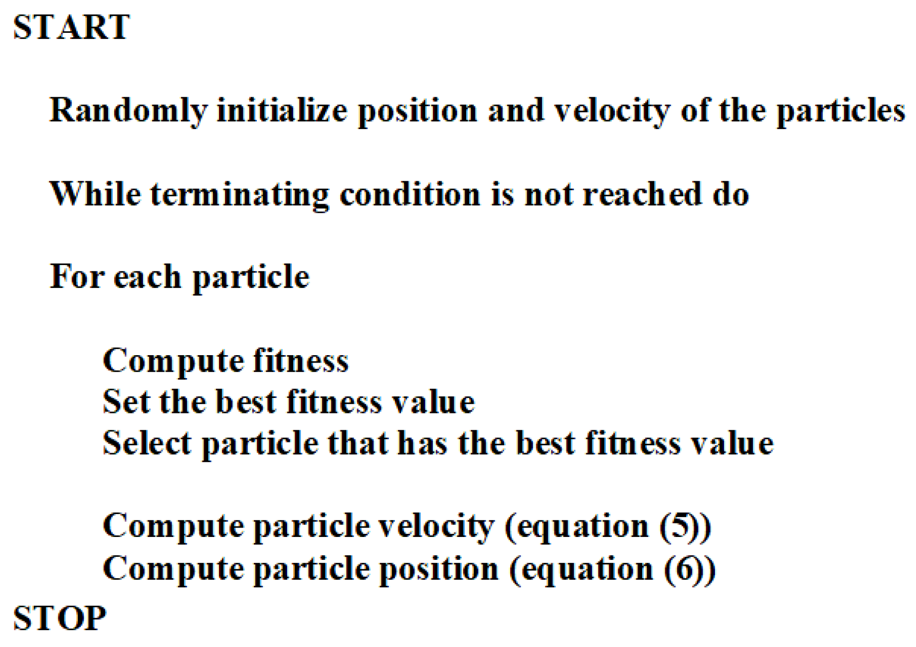
Eberhart and Kennedy introduced the particle swarm optimization (PSO) algorithm in the mid-nineties [17]. The PSO is a population-based search algorithm inspired by the social behaviors of animals or insects, for instance, the case of bird flocking. The main difference between PSO and the evolutionary strategies is in how each possible solution or particle in the population (swarm) is manipulated [18]. Evolutionary operators such as crossover and mutation are not considered in this approach. Instead, the position of a particle (individual) in a PSO is modified based on the particle’s velocity, its previous best position identified individually thus far, and the previous best positions observed by the remaining particles. Here, velocity and position are the attributes of each particle. This method attempts to replicate the simple behavior of an individual imitating its own success, as well as that of neighboring individuals. When considered in a collective manner comprising all the particles, such behavior leads to the discovery of optimal regions in search spaces with high dimension. Figure 3b and Figure 5 illustrate the steps involved in this strategy, and the updates in the velocity and position of the particles are described in Equations (5) and (6), respectively.
with xi(0) ~ U(xmin, xmax).
vi(n) is the velocity of particle i at iteration number n, similarly, xi(n) represents the position of particle i at n; C1 and C2 denote positive constants usually referred to as cognitive and social factors, respectively, and Rand1() and Rand2() are random values in the range [0,1]. U() signifies the bounds of the particles. The best position of particle i since the first iteration and the best position discovered by any of the particles so far are expressed by Pi and PN, respectively. Ω is a relaxation factor that helps in convergence, assigned a value of 0.8. C1 in the present context is set to 1.50 and C2 also has a value of 1.50. In the PSO, the population (swarm) is initialized randomly (within specified bounds), and subsequently each particle is evaluated using an objective function and the particle position to determine the best individual position and the global best position. Once the termination criterion has been verified and if no further iterations are required, the velocities and positions of all the particles are updated using the above relations.
3.3. Differential Evolution
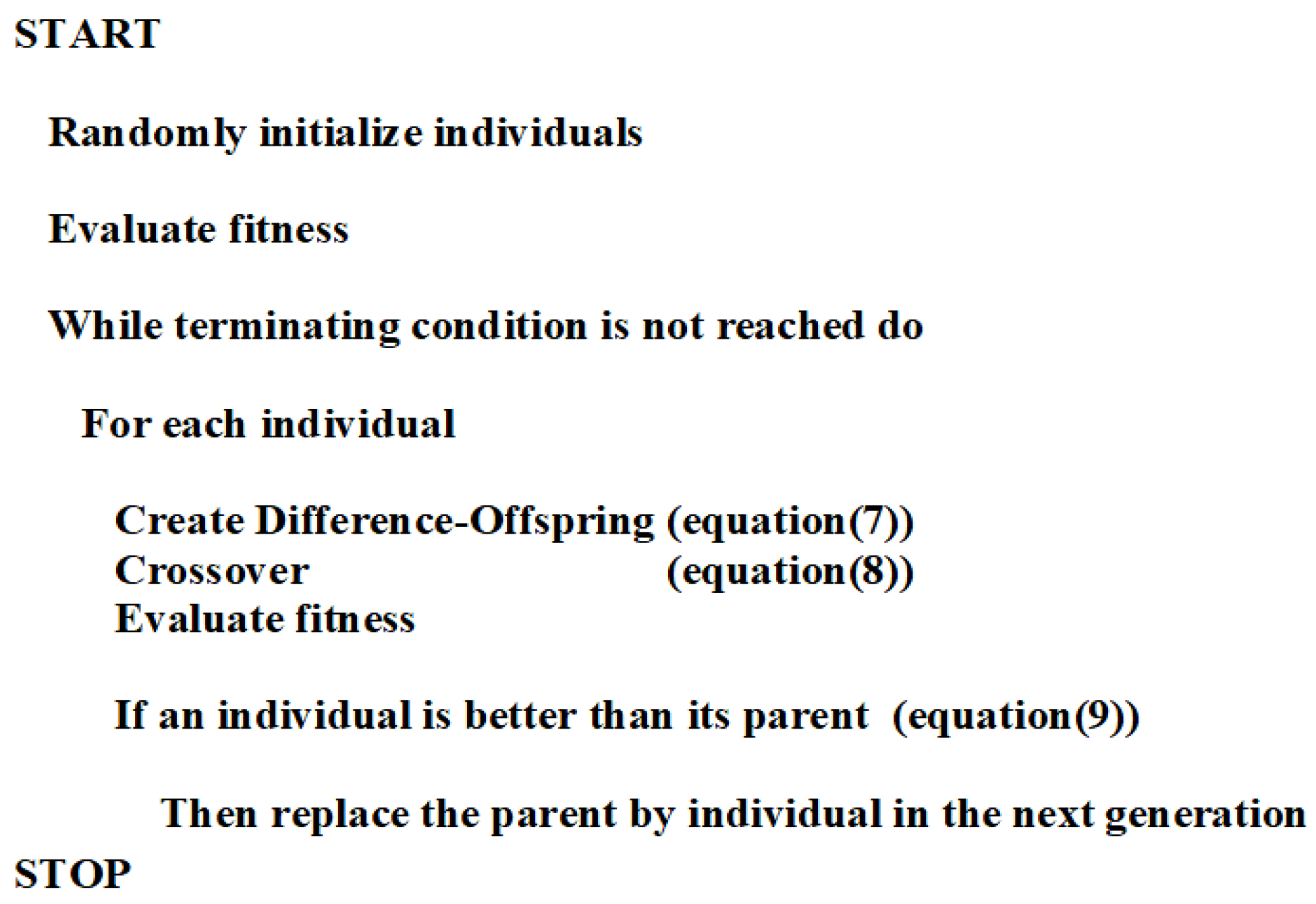
Differential evolution (DE) is similar to the GA, as it also belongs to the family of evolutionary algorithms and it applies mutation and crossover operators [19,20,21]. Developed by Kenneth Price and Rainer Storn, DE involves vector-based operations. Figure 3c and Figure 6 present the procedures applied in this strategy. Unlike the GA, the manipulations here do not occur at a specific section or an individual part of a chromosome. Instead, in DE all the vectors (individuals) are considered. For instance, Equation (7) explains the case of mutation where three distinct vectors are first randomly sampled from the population. Subsequently, the difference between the two vectors (from the set of three) is scaled using F to perturb the third vector in order to create a mutant vector (Pν,G). Similarly, for the crossover shown in Equation (8), either the mutant or the parent vector (Xν,G) is picked as a trial vector (Uν,G) based on the crossover rate (Cr), and no swapping of a section of the vector is involved as prevalent in GA. Finally, in the selection process, the parent vector is replaced if the trial vector delivers an objective function value that is less than that obtained by the parent vector; otherwise, the former is retained. The population size remains constant after each generation.
In the above relations, G denotes the generation, the index r represents different vectors (individuals) from the population, obj is the objective function, and ν indicates distinct base vectors. The control parameters F and Cr are assigned the values of 0.9 and 0.5, respectively. Recent trends in DE are provided in [16,22,23].
4. The Surrogate-Assisted Non-Deterministic Algorithm
Compared to the classical approaches, non-deterministic methods are more robust and can better deal with the moderate noise and multi-modality present in a search space. However, the large number of function calls associated with non-deterministic techniques combined with finite element evaluations at every call can significantly increase the computational cost. Surrogate modeling is an effective mechanism to address this issue, as expensive simulations can be replaced with inexpensive surrogate models [24]. Polynomial regression, neural networks, Kriging, radial basis function, and support vector machines are the main examples that have widely been applied to generate surrogates. This work restricts itself to the polynomial regression approach because the procedure is both simple and sufficient to address a problem involving five parameters. Figure 7 shows the coupling between a surrogate model and a non-deterministic optimizer; the cycle begins with population initialization and evaluation using the error function. The following subsections describe the polynomial regression fundamentals, present the implementation of the surrogate model for the Romaine-2 dam, and explain how the model was integrated with non-deterministic algorithms.
4.1. Polynomial Regression Model
A regression model identifies the relationship between a dependent and one or more independent variables [25]. In this investigation, the estimated displacements along the INV01 inclinometer are the dependent variables, and the set of five parameters: the shear modulus (G), Poisson coefficient (ν), friction angle (φ), cohesion (c), and specific weight (γ) of the material/soil represent the independent variables. Assuming that the true displacement at a point in the dam (over INV01) due to the influence of vector X composed of the set of independent variables is y, the relationship between the two is defined as:
where ϵ is an error term and f(X)denotes the response. In the real world, f(), in a search space, is unknown, and this necessitates the use of some form of approximation. A simple approach that performs this task is linear regression, which can be expressed in the following manner:
where β0 and βi are the coefficients, m is the dimension (five in the present scenario), and implies the individual parameters. The regression coefficients are calculated by minimizing the residual sum of squares , where n is the number of observations. In situations where there is nonlinearity involved in the design space, linear regression models may not give satisfactory results. Polynomial regression can be a suitable option in such scenarios; it succeeds by extending the ideas applied to fitting a linear regression model. Instead of combining input variables linearly, they are combined by raising them to degrees greater than one, as shown below.
Equation (12) depicts the case of a second-order polynomial model with β0, βi and βij denoting the coefficients; the input variables are represented by xi and xj. The number of coefficients to be estimated increases as the order of the polynomial increases, which in turn requires more sample points and adds to the complexity. Instabilities and unwanted fluctuations may also arise, all of which are major drawbacks of polynomial regression. This work does not delve further into the limitations; however, neural networks have proven to be an effective approach for problems that contain a large number of input variables and display highly nonlinear behavior. [26] provide a good insight into model approximation methods, and try to relate the experimental design, choice of model, number of dimensions and sample points using different examples. Scikit-learn, an open-source machine-learning library in Python, has been used to implement the polynomial-based surrogate model.
4.2. Surrogate Model of Rockfill Dams
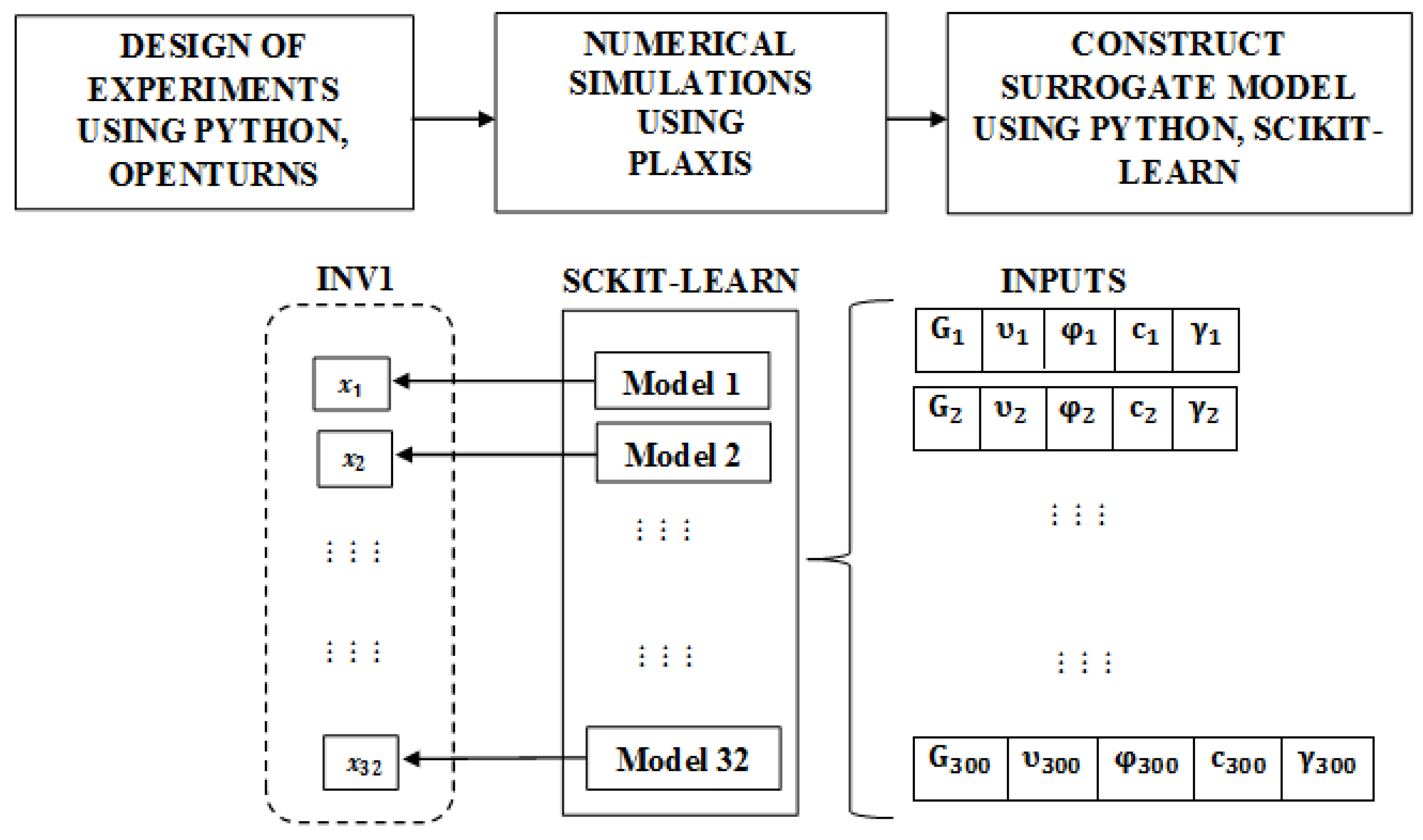
The execution of computer codes is time-consuming, hence identifying the inputs that have the potential to influence results the most is important. The design of experiments attempts to address this aspect by providing a sampling plan for relevant inputs in the design space. This phase forms the first stage of the surrogate modeling process, as shown in Figure 8. This work uses the open-source library OpenTURNS to perform sampling. Special techniques are considered to ensure that the input points are spread evenly throughout the design space without sacrificing efficiency, including the Monte Carlo (MC) method, the Hammersley, Halton, Faure, and Sobol sequences (family of low-discrepancy sequences), and Latin hypercube sampling (LHS) [27].
Over the years, MC methods have become a standard approach for computer-based simulations, and they have been applied successfully in a wide range of problems. However, such techniques are based on random sampling, which may lead to the clustering of sample (input) points, resulting in extraneous and expensive computational runs. Clustering occurs because the points generated randomly lack uniformity and do not always occupy the spaces between already-sampled points. Quasi Monte Carlo (QMC) techniques, also known as low-discrepancy sequences (LDSs) and LHS, are better equipped to generate uniform point distribution. The variance reduction LHS method has been effective in numerous examples, specifically involving lower dimensions (n < 20). Depending on the problem, modified designs of LHS, using optimal space-filling criteria such as the minimax, maxmin approach and the minimum spanning tree strategy, may show some improvement in LHS efficiency. QMC involves deterministic sequences with no random components; the points are generated in a manner that rigorously imposes the concept of uniform coverage of the sampling space. Among the sequences in this category, Sobol LDSs are the most effective, and this work considers them to generate the input parameters for zone P, as shown in Table 1. In a relatively low dimension, studies have demonstrated that the QMC method displays lower discrepancy and higher efficiency when compared with the MC and standard LHS methods [28]. Our investigations in [29] highlight the standard deviation patterns involving different sample sizes using Sobol and LHS for the Romaine-2 problem. The table below presents the different parameter bounds for zone P. Zones O and N have the constant values as specified; for more details refer to [6,10]. These estimates provided a good approximation of the dam’s behavior.
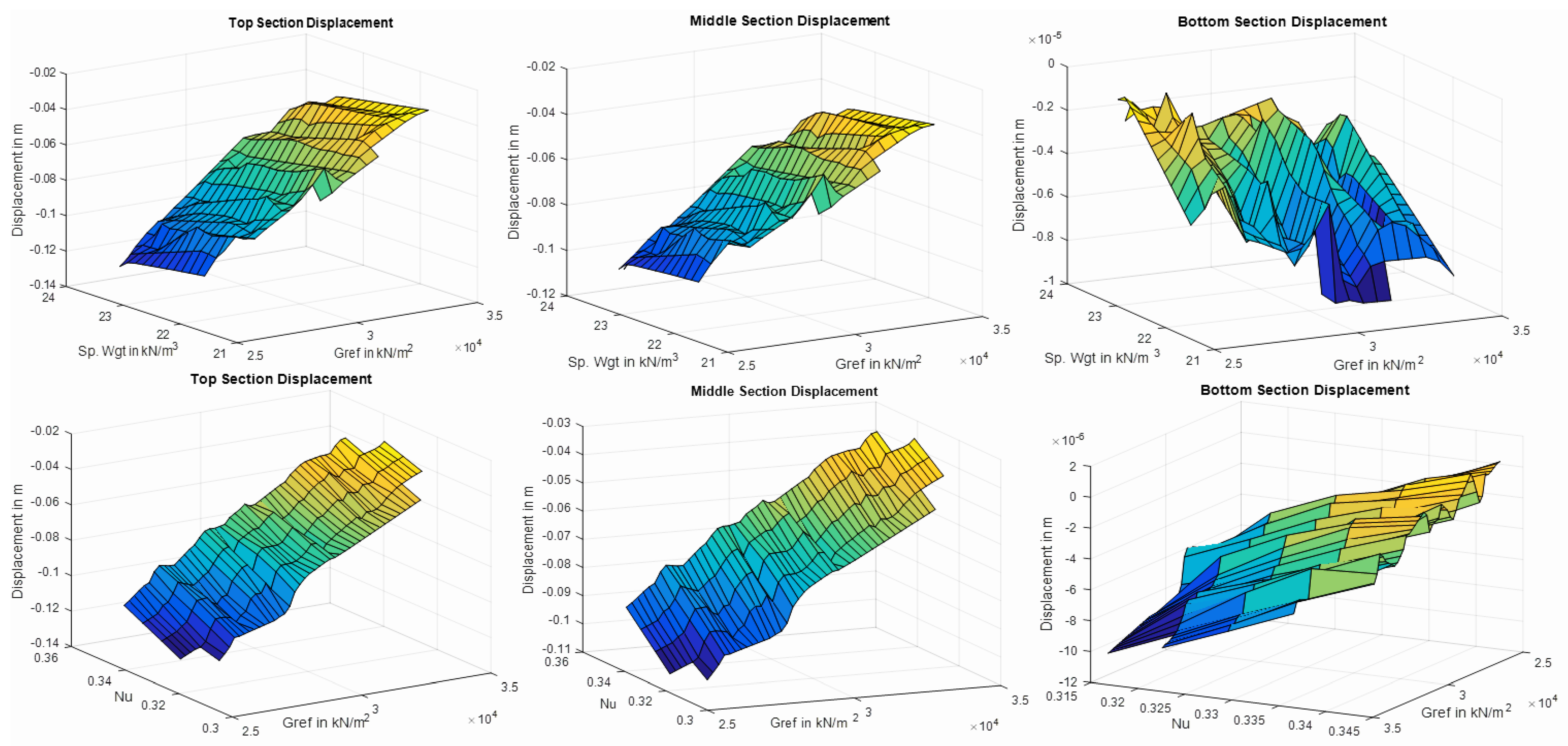
In order to create the surrogate model, 300 sample sets (in Zone P) were generated, where an individual set is comprised of five parameters, each having a value that lies within the specified bounds. The study in [29] indicated that 300 samples are adequate to provide a good representation of the dam’s response (a portion of this sample is provided in Appendix A). Every sample for zone P, along with the parameters for zones O and N, were then used to simulate and solve the Romaine-2 problem in Plaxis, and the corresponding displacements along the coordinates of INV01 were recorded. Figure 9 provides the surface plots of the simulated displacement values displaying the troughs and crescents. The top, middle, and bottom sections are situated at altitudes of 242 m, 190 m, and 144 m, respectively. For additional details, refer to Section 2 and Figure 1.
Using the set of 300 input data and the corresponding displacement values at 32 locations along INV01 (refer to Figure 8), a polynomial regression model was created with the help of the Sckit-learn library. An analysis was also performed to ascertain the polynomial order that provides the most accurate results. Table 2 presents a comparative chart of the polynomial order used and the observed root mean squared error. Obviously, the model of order three provides results that most closely resemble the displacement behavior of the Romaine-2 dam. This model was then used in conjunction with the non-deterministic algorithms to perform the inverse analysis.
5. Simulation Results
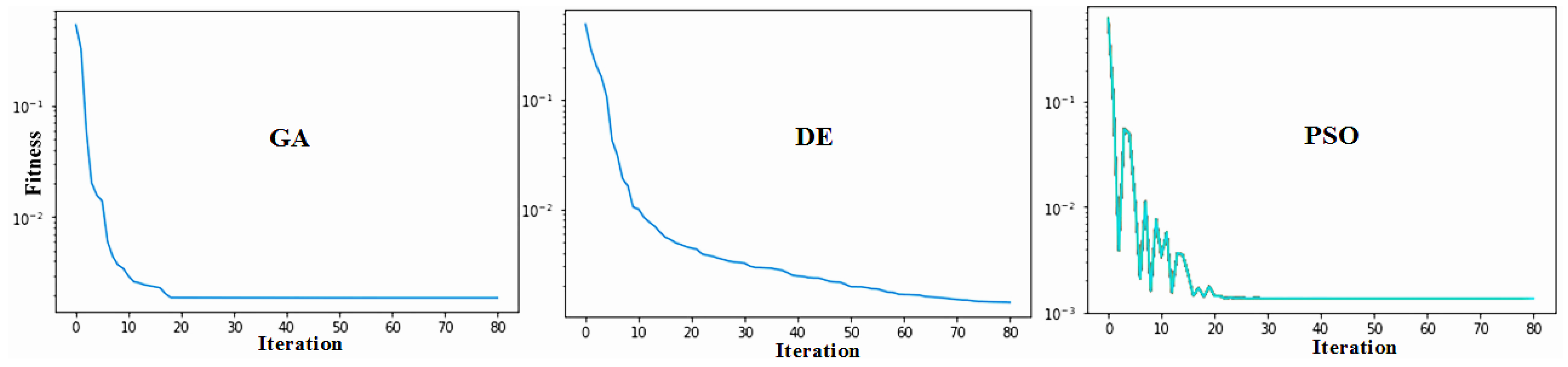
This section presents the inverse analysis outcomes for the Romaine-2 dam problem, using particle swarm optimization (PSO), a genetic algorithm (GA), and differential evolution (DE) approaches. Section 4 described the simulation flow involving these algorithms and the surrogate model, and Section 3 presented the various parameters associated with the algorithms. A trial-and-error approach was performed initially, to estimate the parameters for the algorithms. In order to evaluate the three methods in the present scenario, the population size and the iteration count were varied to analyze the individual convergences. Once they were ascertained, the iteration/generation count was fixed at 80, and the population size for PSO and DE was set to 50, whereas for the GA it was 200. The rationale here is to have an iteration count beyond which no substantial improvement in the convergence is observed in the three cases, and to have a population that achieves this goal without sacrificing efficiency or accuracy. With these objectives, the respective computer programs were executed 10 times (using a 32 GB RAM, Intel-i7 processor compute machine) for each algorithm to determine if there was any significant deviation from the expected convergence behavior and the results. The simulations did not display any major shift from the general trend; the following plots and Table 3 present the observed convergences and the analysis results (the average of all runs), respectively. Figure 10 shows the convergence trend in the three algorithms.
From the above details, it is evident that the PSO and DE provide better fitness values compared to the GA, and that the same two algorithms render similar results. In addition, the GA requires a larger population size compared to the PSO and DE to perform the same analysis. In terms of convergence rate, the GA and the PSO require fewer iterations to reach the optimum fitness value compared to DE. However, there are more parameters to tune in the PSO, whereas there are only two in the GA and in DE. Figure 11 presents a comparison between the simulated displacement using the optimal values found with DE and the displacement recorded by the inclinometer at INV01 (refer to Section 2 for the location of INV01). The significant differences between the results in the higher elevations could be attributed to errors that arise due to extreme variation in temperatures (weather/environment effects) encountered by the inclinometers. Furthermore, the instruments are not always calibrated accurately, which introduces additional sources of errors.
6. Conclusions
The presence of uncertainties has always posed a challenge in the design of rockfill dams, and traditional approaches are not very effective in resolving them. Recent advances in computing power and in the ability of modern instruments to collect data (often in real-time) from rockfill dams have made techniques based on optimization and statistical methods much more attractive. These procedures provide a more realistic picture of a system. The purpose of this research was to present a framework involving optimization and statistical techniques that could be applied to rockfill dams. In the process, this paper investigated the potential of different non-deterministic algorithms, defined a suitable error function (objective function), prescribed a simple approach to construct a surrogate model to reduce the computation cost and a sampling technique to generate such a model. The ideas discussed here can easily be extended to any rockfill dam with known specifications and where displacement data are available.
To demonstrate the effectiveness of the framework, a real-world example was considered, the Romaine-2 dam with its multiple zones carrying different materials. Displacement measurements derived from a vertical inclinometer situated close to the dam core were used to define the error function. In addition, to reduce the oscillations observed in the instrument readings, a correction factor that smooths them was used in the error function. A low-discrepancy sequence in the form of a Sobol procedure was applied to generate uniformly distributed parameter samples. The use of polynomial regression to develop the surrogate model in the present case was recommended, and an analysis that identifies the appropriate order was presented. In order to perform the inverse analysis, three non-deterministic algorithms—the PSO, the GA, and DE—were developed and coupled with the surrogate model. A detailed study was performed to determine the various parameters associated with the three methods, as well as the most suitable population size for each case. This investigation provides a comparison of the three algorithms in the inverse analysis process. The results indicate that in the present scenario, the PSO and DE outperform the GA. Table 1 and Table 3 present an interesting insight: the estimated shear modulus and friction angle values are closer to the assigned upper limits in P, whereas the specific weight is close to the assigned lower limit. The Poisson coefficient estimate is closer to the average of the two bounds.
For future work, an investigation that considers all the zones would help to provide a better understanding of dam behavior. In addition, an analysis that incorporates complex constitutive models, such as the Duncan-Chang and Hardening soil, could be useful. This study is limited to the inclinometer situated in section PM560; analyses involving inclinometers located in other regions of the dam could also provide valuable information. The framework presented here can also be extended to other dams.
Author Contributions
Conceptualization, R.D., A.S.; methodology, R.D.; writing—original draft preparation, R.D.; writing-program scripts, R.D.; writing—review, A.S.; supervision, A.S.; funding acquisition, A.S. All authors have read and agreed to the published version of the manuscript.
Funding
This research was supported by the Natural Sciences and Engineering Research Council of Canada and Hydro-Quebec. Their financial support is gratefully acknowledged.
Institutional Review Board Statement
Not applicable.
Informed Consent Statement
Not applicable.
Data Availability Statement
All data during the study appear in the submitted paper and also the necessary references.
Acknowledgments
The authors express their gratitude to Marc Smith from Hydro-Québec for his valuable comments and suggestions.
Conflicts of Interest
The authors declare that they have no known competing financial interest or personal relationships that could have appeared to influence the work reported in this paper.
Appendix A. Zone P Parameter Set
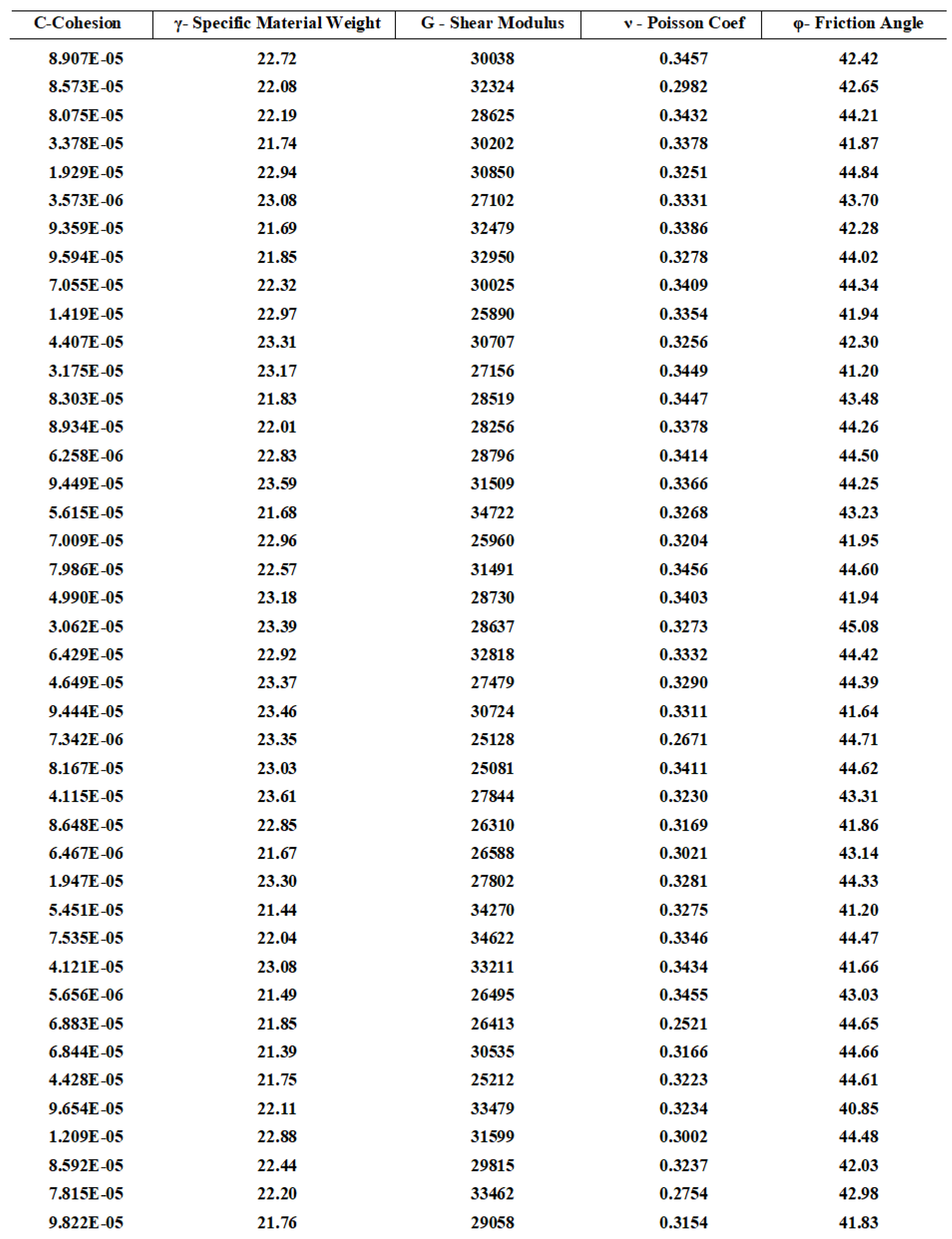
Figure A1 provides only a section of the parameter set generated for zone P. The Sobol LDS procedure was used to generate all the sample points; more details are given in Section 4 and Table 1. As highlighted earlier, 300 samples were produced for the five parameters within the defined ranges.
Figure A1.
Sample points generated by the Sobol LDS approach for zone P. Units: Cohesion—kN/m2; Sp. Material Weight—kN/m3; Friction angle—Degree; Shear modulus—kN/m2.
Figure A1.
Sample points generated by the Sobol LDS approach for zone P. Units: Cohesion—kN/m2; Sp. Material Weight—kN/m3; Friction angle—Degree; Shear modulus—kN/m2.

References
- Holtz, R.D.; Kovacs, W.D.; Sheahan, T.C. An Introduction to Geotechnical Engineering; Pearson: London, UK, 2011. [Google Scholar]
- Bowles, J.E. Foundation Analysis and Design; MacGraw-Hill: Sussex, UK, 1988. [Google Scholar]
- Clough, R.W.; Woodward, R.J. Analysis of Embankment Stresses and Deformations. J. Soil Mech. Found. Div. 1967, 93, 529–549. [Google Scholar] [CrossRef]
- Nocedal, J.; Wright, S.J. Numerical Optimization, 2nd ed.; Springer: New York, NY, USA, 2006. [Google Scholar]
- Coello CA, C.; Lamont, G.B.; Van Veldhuizen, D.A. Evolutionary Algorithms for Solving Mul-Ti-Objective Problems; Springer: Berlin/Heidelberg, Germany, 2007. [Google Scholar]
- Smith, M. Rockfill Settlement Measurement and Modelling of the Romaine-2 Dam during Construction. In Proceedings of the 25th Congress, International Commission on Large Dams, ICOLD, Stavanger, Norway, 15–20 June 2015; Volume 98, pp. 468–485. [Google Scholar]
- Brinkgreve, R.B.J.; Engin, E.; Swolfs, W.M. Plaxis 2D Manual; PLAXIS Inc.: Delft, The Netherlands, 2017. [Google Scholar]
- Baudin, M.; Dutfoy, A.; Iooss, B.; Popelin, A.L. Open Turns: An Industrial Software for un-Certainty Quantification in Simulation. In Handbook of Uncertainty Quantification. arXiv 2015, arXiv:1501.05242. [Google Scholar]
- Schanz, T.; Vermeer, P.; Bonnier, P. The Hardening Soil Model: Formulation and Verification. In Beyond 2000 in Computational Geotechnics; CRC Press: Boca Raton, FL, USA, 2019; pp. 281–296. [Google Scholar]
- Hamed, A.A. Predictive Numerical Modeling of the Behavior of Rockfill Dams. Master’s Thesis, École de Technologie Supérieure, Montreal, QC, Canada, 2016. [Google Scholar]
- Ledesma, A.; Gens, A.; Alonso, E.E. Estimation of Parameters in Geotechnical Backanalysis—I. Maximum Likelihood Approach. Comput. Geotech. 1996, 18, 1–27. [Google Scholar] [CrossRef] [Green Version]
- Holland, J.H. Adaptation in Natural and Artificial Systems; MIT Press: Cambridge, MA, USA, 1992. [Google Scholar]
- Reeves, C.R.; Rowe, J.E. Genetic Algorithms: Principles and Perspectives: A Guide to GA Theory; Springer: Berlin/Heidelberg, Germany, 2006. [Google Scholar]
- Wang, Z.; Sobey, A. A Comparative Review between Genetic Algorithm Uses in Composite Optimi-Zation and the State-of-the-Art in Evolutionary Computation. Compos. Struct. 2020, 233, 111739. [Google Scholar] [CrossRef]
- Liu, J.; Liu, Y.; Shi, Y.; Li, J. Solving Resource-Constrained Project Scheduling Problem via Genetic Algorithm. J. Comput. Civ. Eng. 2020, 34, 04019055. [Google Scholar] [CrossRef]
- Slowik, A.; Kwasnicka, H. Evolutionary Algorithms and Their Applications to Engineering Problems. Neural Comput. Appl. 2020, 32, 12363–12379. [Google Scholar] [CrossRef] [Green Version]
- Chan, F.T.; Tiwari, M.K. Swarm Intelligence, Focus on Ant and Particle Swarm Optimization; I-Tech Education and Publishing: Rijeka, Croatia, 2007. [Google Scholar]
- Cao, Y.; Zhang, H.; Li, W.; Zhou, M.; Zhang, Y.; Chaovalitwongse, W.A. Comprehensive Learning Particle Swarm Optimization Algorithm With Local Search for Multimodal Functions. IEEE Trans. Evol. Comput. 2019, 23, 718–731. [Google Scholar] [CrossRef]
- Price, K.; Storn, R.M.; Lampinen, J.A. Differential Evolution: A Practical Approach to Global Opti-Mization; Springer: Berlin/Heidelberg, Germany, 2006. [Google Scholar]
- Das, R.; Oliveira, F.B.; Guimaraes, F.G.; Lowther, D.A. The Optimal Design of HTS Devices. IEEE Trans. Magn. 2014, 50, 249–252. [Google Scholar] [CrossRef]
- Das, S.; Suganthan, P.N. Differential Evolution: A Survey of the State-of-the-Art. IEEE Trans. Evol. Comput. 2010, 15, 4–31. [Google Scholar] [CrossRef]
- Marek, M.; Kadlec, P. Another Evolution of Generalized Differential Evolution: Variable Number of Dimensions. Eng. Optim. 2020, 1–20. [Google Scholar] [CrossRef]
- Nandi, S.; Janga Reddy, M. Comparative Performance Evaluation of Self-Adaptive Differential Evolution with GA, SCE and DE Algorithms for the Automatic Calibration of a Computationally Intensive Distributed Hydrological Model. h2oj 2020, 3, 306–327. [Google Scholar]
- Queipo, N.V.; Haftka, R.T.; Shyy, W.; Goel, T.; Vaidyanathan, R.; Tucker, P.K. Surrogate-Based Analysis and Optimization. Prog. Aerosp. Sci. 2005, 41, 1–28. [Google Scholar] [CrossRef] [Green Version]
- Jin, R.; Chen, W.; Simpson, T.W. Comparative Studies of Metamodelling Techniques under Multi-Ple Modelling Criteria. Struct. Multidiscip. O 2001, 23, 1–13. [Google Scholar] [CrossRef]
- Keane, A.; Forrester, A.; Sóbester, A. Engineering Design via Surrogate Modelling: A Practical Guide; American Institute of Aeronautics and Astronautics: West Sussex, UK, 2008. [Google Scholar]
- Damblin, G.; Couplet, M.; Iooss, B. Numerical Studies of Space-Filling Designs: Optimization of Latin Hypercube Samples and Subprojection Properties. J. Simul. 2013, 7, 276–289. [Google Scholar] [CrossRef] [Green Version]
- Das, R.; Soulaïmani, A. Global Sensitivity Analysis in the Design of Rockfill Dams. In Proceedings of the Sustainable and Safe Dams around the World, Ottawa, ON, Canada, 9–14 June 2019; Apple Academic Press: Cambridge, MA, USA, 2019; pp. 950–962. [Google Scholar]
- Kucherenko, S.; Albrecht, D.; Saltelli, A. Exploring Multi-Dimensional Spaces: A Comparison of Latin Hypercube and Quasi Monte Carlo Sampling Techniques. arXiv 2015, arXiv:1505.02350. [Google Scholar]
Figure 1.
2D cross-section model of the Romaine-2 dam in Plaxis. Different zones of the dam are highlighted by letters. The vertical inclinometer INV1 is found in section PM560.
Figure 1.
2D cross-section model of the Romaine-2 dam in Plaxis. Different zones of the dam are highlighted by letters. The vertical inclinometer INV1 is found in section PM560.

Figure 2.
Measurements recorded by INV01 prior to the start of impoundment, denoted by the dotted line. These denote horizontal movements; a negative value indicates upstream movement.
Figure 2.
Measurements recorded by INV01 prior to the start of impoundment, denoted by the dotted line. These denote horizontal movements; a negative value indicates upstream movement.

Figure 3.
Flow diagrams of the algorithms considered. (a) GA, (b) PSO, and (c) DE represent the different steps associated with each of the three non-deterministic algorithms.
Figure 3.
Flow diagrams of the algorithms considered. (a) GA, (b) PSO, and (c) DE represent the different steps associated with each of the three non-deterministic algorithms.

Figure 4.
Pseudocode of genetic algorithm considered.

Figure 5.
Pseudocode of particle swarm optimization algorithm.

Figure 6.
Pseudocode of differential evolution algorithm.

Figure 7.
The cycle associated with the surrogate-assisted non-deterministic approach.

Figure 8.
Steps involved in generating a surrogate model of a rockfill dam. Thirty two evenly distributed locations along the inclinometer were considered for the analysis. A set of five parameters was used to generate the 300 input points. These inputs were used to create the regression models for the 32 locations using the Sckit-learn package and the actual displacement values at these locations.

Figure 9.
Displacements at different sections of the dam along INV01. Specific weight, shear modulus, and Poisson coefficient were considered to plot the results. Surface plot representation at different elevations here provide an insight into the nature of the optimization problem at hand.
Figure 9.
Displacements at different sections of the dam along INV01. Specific weight, shear modulus, and Poisson coefficient were considered to plot the results. Surface plot representation at different elevations here provide an insight into the nature of the optimization problem at hand.

Figure 10.
Convergences observed in the analysis using three different algorithms: the GA, DE, and the PSO.
Figure 10.
Convergences observed in the analysis using three different algorithms: the GA, DE, and the PSO.

Figure 11.
Measurements recorded at INV01 by the inclinometer are denoted by the dotted line. The solid line represents the simulated displacement using the optimal parameter values obtained with DE.
Figure 11.
Measurements recorded at INV01 by the inclinometer are denoted by the dotted line. The solid line represents the simulated displacement using the optimal parameter values obtained with DE.


Table 1.
Parameter values in different dam zones.
| P | N | O | |||
|---|---|---|---|---|---|
| Parameters | Upper Limit | Lower Limit | Units | ||
| Shear Modulus | 35,000 | 25,000 | 170,000 | 110,000 | kN/m2 |
| Friction Angle | 45.15 | 40.85 | 47 | 45 | Degree |
| Cohesion | 0 | 0 | 0 | 0 | kN/m2 |
| Poisson Coefficient | 0.3465 | 0.234 | 0.33 | 0.22 | |
| Sp. Material Weight | 23.625 | 21.375 | 23.7 | 22.5 | kN/m3 |
Table 2.
The polynomial order used in the regression model and the corresponding root mean squared error.
Table 2.
The polynomial order used in the regression model and the corresponding root mean squared error.
| Order | RMSE |
|---|---|
| 1 | 0.001597 |
| 2 | 0.000166 |
| 3 | 0.00018 |
| 4 | 0.000152 |
| 5 | 0.000205 |
Table 3.
Values obtained using three different algorithms for the parameters in zone P using the inverse analysis procedure. The fitness value is the error function calculated for the entire population.
Table 3.
Values obtained using three different algorithms for the parameters in zone P using the inverse analysis procedure. The fitness value is the error function calculated for the entire population.
| Algorithm | G(kN/m2) | γ(kN/m3) | φ | v | c | Fitness Value |
|---|---|---|---|---|---|---|
| DE | 3.500 × 10⁴ | 2.138 × 101 | 4.515 × 101 | 3.146 × 10⁻¹ | 0.000 | 0.001 |
| GA | 3.345 × 10⁴ | 2.143 × 101 | 4.193 × 101 | 3.206 × 10⁻¹ | 2.442 × 10⁻⁶ | 0.003 |
| PSO | 3.500 × 10⁴ | 2.138 × 101 | 4.515 × 101 | 3.147 × 10⁻¹ | 0.000 | 0.001 |
Publisher’s Note: MDPI stays neutral with regard to jurisdictional claims in published maps and institutional affiliations. |
© 2021 by the authors. Licensee MDPI, Basel, Switzerland. This article is an open access article distributed under the terms and conditions of the Creative Commons Attribution (CC BY) license (https://creativecommons.org/licenses/by/4.0/).
Share and Cite
MDPI and ACS Style
Das, R.; Soulaimani, A. Non-Deterministic Methods and Surrogates in the Design of Rockfill Dams. Appl. Sci. 2021, 11, 3699. https://0-doi-org.brum.beds.ac.uk/10.3390/app11083699
AMA Style
Das R, Soulaimani A. Non-Deterministic Methods and Surrogates in the Design of Rockfill Dams. Applied Sciences. 2021; 11(8):3699. https://0-doi-org.brum.beds.ac.uk/10.3390/app11083699
Chicago/Turabian StyleDas, Rajeev, and Azzedine Soulaimani. 2021. "Non-Deterministic Methods and Surrogates in the Design of Rockfill Dams" Applied Sciences 11, no. 8: 3699. https://0-doi-org.brum.beds.ac.uk/10.3390/app11083699
Note that from the first issue of 2016, this journal uses article numbers instead of page numbers. See further details here.