
Constructing 3D Underwater Sensor Networks without Sensing Holes Utilizing Heterogeneous Underwater Robots


Electronic and Electrical Convergence Department, Hongik University, Sejong 2639, Korea
Appl. Sci. 2021, 11(9), 4293; https://0-doi-org.brum.beds.ac.uk/10.3390/app11094293
Submission received: 22 April 2021
/
Revised: 5 May 2021
/
Accepted: 7 May 2021
/
Published: 10 May 2021
(This article belongs to the Special Issue Advances in Robot Path Planning)
Abstract
:This article handles building underwater sensor networks autonomously using multiple surface ships. For building underwater sensor networks in 3D workspace with many obstacles, this article considers surface ships dropping underwater robots into the underwater workspace. We assume that every robot is heterogeneous, such that each robot can have a distinct sensing range while moving with a distinct speed. The proposed strategy works by moving a single robot at a time to spread out the underwater networks until the 3D cluttered workspace is fully covered by sensors of the robots, such that no sensing hole remains. As far as we know, this article is novel in enabling multiple heterogeneous robots to build underwater sensor networks in a 3D cluttered environment, while satisfying the following conditions: (1) Remove all sensing holes. (2) Network connectivity is maintained. (3) Localize all underwater robots. In addition, we address how to handle the case where a robot is broken, and we discuss how to estimate the number of robots required, considering the case where an obstacle inside the workspace is not known a priori. Utilizing MATLAB simulations, we demonstrate the effectiveness of the proposed network construction methods.
1. Introduction
Sensor networks can perform various autonomous tasks in dangerous and harsh environments. In the case where each sensor has mobility, sensor network can perform environmental monitoring [1,2,3], area coverage [4,5,6,7], formation control [8,9,10], target tracking [11,12], or intruder detection [13,14,15,16].
This article solves the coverage problem using multiple mobile sensors in an underwater cluttered environment. A mobile sensor needs to avoid underwater obstacles while it moves, since we consider 3D underwater environments with many obstacles. Underwater mobile sensors are deployed in the workspace, to perform collaborative monitoring and data collection tasks. For complete monitoring of the cluttered workspace, it is required to build sensor networks such that no sensing hole exists in the workspace.
In underwater environments, optic, electromagnetic, or acoustic sensors have been used for wireless communication [17,18]. But, building sensor networks in underwater environments is difficult, since communication range is rather short [19,20,21].
As a method to build underwater sensor networks autonomously, this article considers surface ships dropping underwater robots into the underwater 3D workspace. Here, each robot can move and has sensing/communication abilities. Since Global Positioning Systems (GPS) cannot be used to localize an underwater robot, this article introduces network building approaches to generate underwater sensor networks, while localizing every robots in the networks.
As a ship arrives at the sea surface of the designated workspace, it begins dropping underwater robots while not moving at the site. Once multiple robots are dropped, they autonomously move into the unknown 3D cluttered workspace until no sensing hole exists in the workspace. As a robot moves in a cluttered workspace, it needs to avoid obstacles while maintaining the network connectivity with other robots.
Many papers handled how to make multiple robots perform area coverage in 2D environments [4,5,8,22,23]. To build a sensor network in an unknown 2D workspace, the reference [2] made a single robot explore the workspace while deploying static sensor nodes. One restriction of this approach is that the robot must be large enough to carry all sensor nodes. Also, the robot must have enough power to explore the 2D workspace completely, since a sensor node has no mobility. the references [6,7] used Voronoi tessellations to make all robots spread in order to increase network coverage based on distributed information from their neighbors. The authors of [8] considered deploying a swarm of robots into an unknown 2D environment to remove all sensing holes in the environment. The authors of [8] handled the case where each robot has bearing-only sensors measuring the bearing to its neighbor in its local coordinate frame. Cluttered environments were not considered in the papers addressed in this paragraph.
Our paper is distinct from other papers addressed in the previous paragraph, since our paper considers the coverage problem in 3D workspace with many obstacles. Since a robot moves in a cluttered workspace, it needs to avoid obstacles while building the sensor network.
As far as we know, only a few papers handled coverage path planning for 3D space. In [24], different deployment strategies for 2D and 3D communication architectures for UnderWater Acoustic Sensor Networks (UW-ASNs) were proposed. For deploying underwater sensors, the reference [24] introduced a sensor which is anchored to the sea bottom and is equipped with a floating buoy that can be inflated by a pump. The buoy pulls the sensor towards the ocean surface. The depth of the sensor can then be regulated by adjusting the length of the wire that connects the sensor to the anchor. However, this deployment approach cannot be used for covering a deep sea. Also, collection of these sensors is not trivial, since a sensor is anchored to the sea bottom. Moreover, the deployment strategy in [24] does not assure that all coverage holes are removed after the deployment.
In this paper, we consider a robot which can freely move in 3D underwater environments. Under the proposed deployment strategy, all robots are deployed so that no sensing holes exist in the workspace. Suppose that a coverage mission of the underwater network is done. In this case, we need to gather the robots, so that they can be deployed for coverage of another space. By controlling the buoyancy of each robot, we can easily make each robot move to the sea surface. Then, a ship can collect the robots easily.
The references [25,26] handled 3D coverage path planning (i.e., path planning process for enabling full coverage of a given 3D space by one or multiple robots). The goal of such planning is to provide nearly full coverage, minimizing the occurrence of visiting an identical area multiple times. However, the references [25,26] did not address how to deploy autonomous sensors, so that the 3D workspace is continuously monitored by the deployed sensors. In our paper, we develop coverage control so that once the robots are located at their designated target positions, then the 3D workspace is continuously monitored by the deployed robots.
In practice, a robot may not be identical to another robot. For instance, some robots may not move as fast as other robots, since their hardware systems are partially broken during their operations. Hence, we assume that every robot moves with a distinct speed. Moreover, a robot may have a distinct sensing range with another robot. Hence, this article assumes that every robot is heterogeneous, such that each robot can have a distinct sensing range while moving with a distinct speed. This article thus handles a scenario where heterogeneous robots are deployed in unknown underwater environments.
Since obstacles can block the communication link between robots, each robot is controlled while maintaining the network connectivity in obstacle-rich environments. The proposed coverage methods work by moving a single robot at a time to spread out the 3D sensor network, until the 3D workspace is fully covered without sensing holes.
The surface ships dropping robots can use GPS to localize themselves. However, GPS cannot be used for localization of a robot. This article assumes that a robot can calculate the relative location of its neighboring robot using local sonar sensors. In underwater environments, sonar sensors are preferred, since sonar signal can travel a longer distance, compared to electromagnetic wave [18]. The proposed coverage methods result in underwater sensor networks without sensing holes, while localizing all robots.
As far as we know, this article is novel in enabling multiple heterogeneous robots to build underwater sensor networks in a 3D cluttered environment, while satisfying the following conditions:
- remove all sensing holes.
- network connectivity is maintained.
- localize all underwater robots.
This paper further addresses how to handle the case where a robot is broken. Also, we address how to conjecture the number of robots required, considering the case where an obstacle inside the 3D workspace is unknown a priori. Utilizing MATLAB simulations, we demonstrate the effectiveness of the proposed coverage methods.
The article is organized as follows: Section 2 introduces the preliminary information of this article. Section 3 introduces the 3D coverage methods utilizing multiple heterogeneous robots. Section 4 shows the MATLAB simulations of the proposed 3D coverage methods. Section 5 presents the discussion on the paper. Section 6 discusses conclusions.
2. Preliminary Information
2.1. Problem Statement
This article solves the space coverage problem using multiple robots in underwater environments. For complete monitoring of the given 3D workspace, it is required to build sensor networks such that no sensing hole exists in the given workspace.
Initially, all robots are carried by surface ships. Here, each robot has both sensing and communication abilities. As a ship arrives at the sea surface of the workspace, it begins dropping robots while not moving at the site.
The dropped robots move autonomously until the 3D workspace is fully covered by sensors of the robots. The obstacles in the workspace are unknown to each robot, and every robot moves based on local interaction with its neighboring robot. Our coverage methods result in underwater sensor networks without sensing holes, while localizing all robots. Section 3 discusses the 3D coverage methods using multiple robots.
2.2. Assumptions and Notations
Using the notations in graph theory [27], a weighted directed graph G is a set , in which is the node set and is the directed edge set. The weight of every directed edge, say , is . A directed path is a sequence of directed edges.
Suppose that we have S surface ships in total. Let denote the s-th surface ship where . Each surface ship carries robots in total.
As a ship arrives at the sea surface of the workspace, it begins dropping robots while not moving at the site. Let denote the i-th robot dropped by . Since carries robots, we have . The ship drops robots in the following order: .
Suppose that each robot has both Ultra-Short BaseLine acoustic positioning (USBL) and depth sensors. USBL sensors can be used to derive both the range and the azimuth of a signal source. USBL sensors can also be used for mutual communication, i.e., a transmitter can send data to a receiver. Each USBL sensor can work as a transmitter as well as a receiver. For instance, one can access the information on commercial USBL sensors in the following website: https://www.ixblue.com/products/usbl-positionning-system (accessed on 10 May 2021).
Let represent the detection (sensing) range of . Also, let represent the communication range of . Let detect-communicate range be defined as
Let of a robot define a sphere with radius , whose center is located at . Let of a robot indicate the boundary of the of the robot.
Let denote the 3D coordinates of where . If , then can sense . Also, can send a communication signal to .
On the of a robot , Q points are evenly generated. These points represent the points where the sensing ray of can reach.
As an example, we discuss generating points on a of a robot. (This generation method is utilized in Section 4.) Let us rotate one vector by about the z-axis. The matrix presenting the rotation is
Thereafter, we rotate by about the y-axis. The matrix presenting the rotation is
The resulting vector after two rotations is
The vector represents the relative position of a point on the of , with respect to . As we add to , we obtain the 3D coordinates of a point on the of . Note that and are chosen from 18 values, respectively. Therefore, points are derived on of .
Let denote a straight line segment connecting two robots and . We say that is safe once it does not intersect an obstacle. This implies that a robot avoids colliding with an obstacle, as it travels along .
A freePoint of denotes a point among Q points of , such that a straight line segment connecting and the point does not intersect obstacles. In practice, freePoints can be detected by active sonar sensors. A robot has active sonars, which can detect an obstacle close to the robot [28].
The authors of [28] considered the case where the active sonars are positioned, so that the viewing angle of the sonars is 200 degrees. In our paper, we need to install active sonars surrounding the robot. In this way, the sonars can cover the space surrounding the robot. As a sonar ray does not meet an obstacle, the ray is associated to a freePoint of the robot.
A frontierPoint of a robot denotes a freePoint of , which is outside the of any other robot. As , one obtains dense frontierPoints on a . Let frontierSurface denote the set of frontierPoints as .
A frontierSurface is on the border between a space covered by all s and a space covered by no . If every robot has no frontierSurface, then all robots’ s cover the open space completely.
Recall that denotes the i-th robot which is dropped by the ship (). Each robot stores and expands the traversible graph, say . Each vertex in indicates a deployed robot. Every directed edge, say , is established as the following conditions are met:
- is safe.
- .
Using the above definition, implies that can detect . Also, can send a communication signal to . is accessible using USBL sensors.
Suppose that a new robot, say , is deployed in , so that this new robot and a robot, say , in satisfy the following two conditions for establishing a directed edge.
- is safe.
- .
In this case, a new directed edge is established from to . Then, and merge to generate the bigger graph . In this way, can expand to contain a robot which is dropped by a ship where .
In the case where is not connected to , and expand independently to each other. Once is connected to , they merge to generate the bigger graph .
Utilizing the notation of , avoids collision while traversing an edge in . This implies that is a safe topological map for .
The weight of every directed edge, say , is . is accessible using USBL sensors and is set as . The weight of every edge in is used to let find the path in .
We say that two robots and are neighbors in the case where . Let denote a neighbor of .
We assume that a ship dropping robots can localize itself using GPS. In summary, every robot satisfies the below assumptions:
- (A1)
- Using the local sonar sensor of a robot n, n is able to calculate the relative location of its neighbor robot .
- (A2)
- A robot n is able to access , the detect-communicate range, of its neighbor robot .
- (A3)
- A robot n is able to calculate the relative location of a frontierPoint in .
2.3. Each Robot Uses USBL and Depth Sensors to Enable Assumptions (A1) and (A2)
Suppose that a robot n transmits a signal to another robot, say . The bearing of the signal is measured by the USBL of m. The signal bearing is measured by the USBL of m, which contains an array of transducers. The transceiver head normally contains three or more transducers separated by a baseline of 10 cm or less. A method called “phase-differencing” within this transducer array is used to calculate the signal direction. The equation for bearing measurement is
Here, . Furthermore, indicates the j-th element in . In (5), indicates the bearing measurement noise. In (5), define the angle of a complex number, say .
Suppose that a robot n transmits a signal to another robot, say . Then, m replies with its own acoustic pulse. This return pulse is detected by n. The time from the transmission of the initial acoustic pulse until the reply is detected is measured by the USBL system of n and is converted into a range. This is feasible, since n has the reference system to measure the signal speed in underwater environments. This range estimation is then shared by both n and m.
The equation for range measurement between n and m is
Here, indicates the range measurement noise.
Note that m has depth sensors to measure its depth. The depth of m is measured using
Here, indicates the depth measurement noise. Also, indicates the third element in . We define
Then, the relative position of n with respect to m is
USBL sensors can be used to transmit information from a transmitter to a receiver. Hence, the relative position information in (9) can be shared by both m and n. Moreover, information of m and n can be shared by two robots. Thus, Assumptions (A1) and (A2) hold.
We next calculate the number of communication pings required, so that two neighboring robots m and n can share the relative position information. The bearing measurement in (5) requires a single communication ping from n to m. The range measurement in (6) further requires a return pulse from m to n. Then, the calculated range measurement is sent from n to m. Also, the bearing measurement in (5) is sent from m to n. In total, four communication pings are required, so that two neighboring robots m and n can share the relative position information.
2.4. Each Robot Uses Active Sonars to Enable Assumption (A3)
Recall that a frontierPoint of a robot n denotes a freePoint of n, which is outside the of any other robot. A robot n can detect an obstacle close to it using its local active sonar sensors. A robot has active sonars, which can sense an obstacle close to the robot [28]. Thus, a robot can calculate the relative location of its freePoint.
Moreover, n can derive the relative location of its neighbor robot using Assumption (A1). Note that n has neighbors. Hence, communication pings are required, so that n and every robot in can share the relative position information.
Furthermore, using Assumption (A2), n can access the detect-communicate range of its neighbor in . communication pings are required for this access. In summary, communication pings are required, so that n can access both the relative position and the detect-communicate range of its every neighbor in .
Thus, n can find a freePoint, which is outside the of any other robot. In other words, n is able to calculate the relative location of a frontierPoint in . Hence, Assumption (A3) is derived. Note that communication pings are required to calculate the relative location of a frontierPoint in .
3. Coverage Methods Utilizing Multiple Heterogeneous Robots
This section handles the following problem: Consider surface ships dropping multiple heterogeneous robots. Build 3D sensor networks without sensing holes, while localizing all robots. While each robot moves, it satisfies the following aspects: obstacle avoidance, and network connectivity are preserved.
To solve the above problem, this article proposes the coverage methods (Algorithm 1) as follows. Initially, all robots are dropped by a surface ship on the sea surface of the 3D workspace. Then, every robot is controlled one after one sequentially, such that as we locate more robots at their designated target positions, an unsensed open space reduces gradually. The proposed coverage algorithm works by moving a single robot at a time to spread out the sensor network, starting from an initial site and spreading out to cover the workspace completely.
Suppose a robot reaches its designated target position (see Algorithm 1). Thereafter, the robot activates its local sonar sensors to sense its surroundings. To build a connected network, a robot moves into an unsensed open space within distance units. As a robot reaches its designated target position , the robot activates its local sonar sensors with range .
| Algorithm 1 Coverage methods using a ship . |
|
In Algorithm 1, every robot is controlled one after one sequentially. Initially, activates its active sonar sensors to sense an obstacle close to the robot. Thus, can calculate the relative location of its freePoint. Thereafter, frontierPoints of are generated. Since is the robot which is deployed for the first time, it has no neighbors when it generates frontierPoints. Therefore, no communication pings are required to calculate the relative location of a frontierPoint in .
Whenever a new robot, say n, is dropped by a ship, n moves until arriving at the nearest frontierPoint. The robot n then activates its local sonar sensors to sense its surroundings. FrontierPoints of n are generated accordingly. Note that communication pings are required to calculate the relative location of a frontierPoint in . Repeat this until every robot is positioned at its designated target position.
Recall that robots are dropped in the following order: . Consider the case where just activated its local sonar sensors to sense its surroundings. The robot finds the nearest robot, say m, with a frontierPoint. The directed breadth-first search can be used for finding m. The time complexity of the directed breadth-first search is , since every edge will be explored in the worst case.
One frontierPoint on m is then chosen as . Based on the directed breadth-first search, travels along a directed path, say P, in to arrive at m. Recalling the notation of , P is a safe path for . Furthermore, the length of every straight line segment of P is shorter than .
As arrives at a robot in the path P, can move towards the next robot in the path P under Assumption (A1). GPS is not required for this local maneuver. In order to traverse the path P, utilizes local interaction with a robot in P. As arrives at a robot, say , in P, lets access the next robot in P. This information sharing is possible under Assumption (A1).
As arrives at the last robot in the path P, can move towards under Assumption (A3). After arrives at , activates its local sonar sensors to sense its surroundings.
Once activates its local sonar sensors, several frontierPoints inside the of are deleted. This deletion is possible based on local interaction of .
We explain the deletion process in detail. Suppose that a point in is inside the of . Since the relative distance between and a point in is , is a neighbor to . Under Assumption (A1), calculates the relative location of .
Suppose that calculates the relative location of . The relative vector from to a point in is derived by adding the below two vectors, which are available based on Assumptions (A1) and (A3):
- 1
- the vector from to the point in .
- 2
- the vector from to .
As activates its local sonar sensors, several frontierPoints inside the of are deleted. Recall that communication pings are required to calculate the relative location of a frontierPoint in .
Then, broadcasts the deletion of frontierPoints to every other robot which can communicate with using multi-hop communication. Here, multi-hop communication is feasible using USBL of each robot.
This broadcast of requires communication pings, since there are nodes in . Using Algorithm 1, increases from 1 to . Therefore, the number of broadcast pings is .
Also, transmits a signal to the ship via multi-hop communication using USBL, so that the ship can deploy the next robot . finds the nearest frontierPoint. Then, travels along until arriving at the frontierPoint. This repeats until in Algorithm 1.
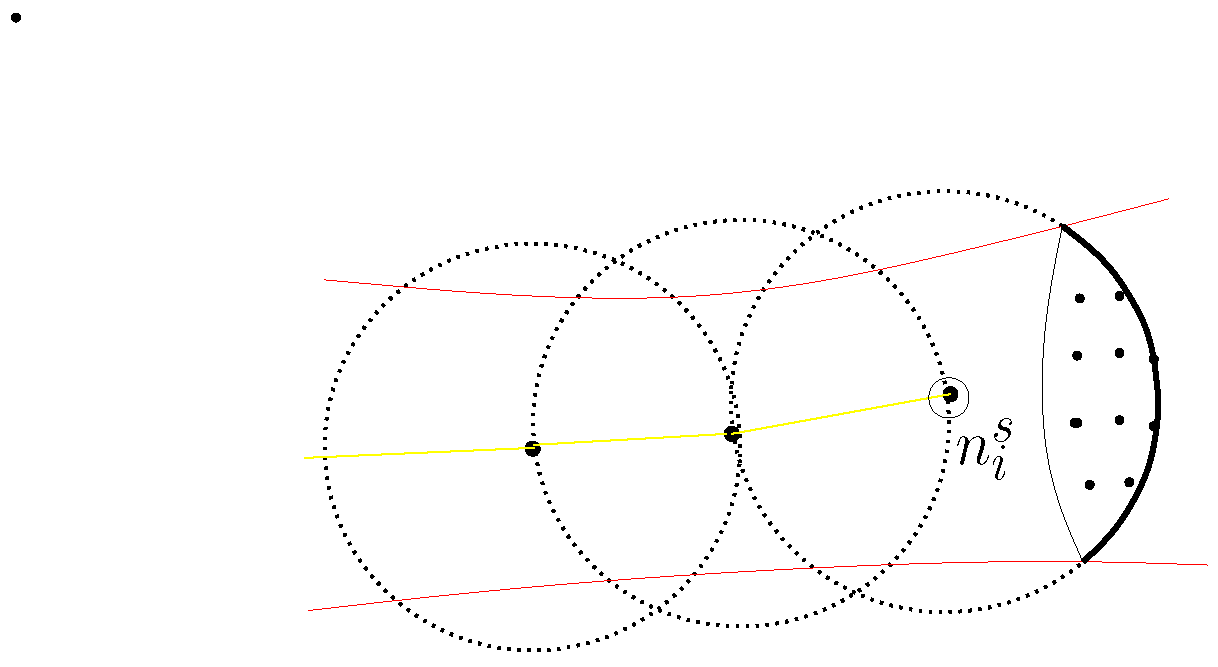
Figure 1 illustrates the case where heads towards . In this figure, is illustrated as a sphere. travels along a narrow passage in Figure 1. Red curves indicate the obstacle boundaries, and the path of is illustrated with yellow line segments. The large dots indicate the robots which are already at their target positions. of every robot is illustrated as a sphere. FrontierPoints are depicted as points on one robot’s .
3.1. Analysis
Algorithm 1 ends when or finds no frontierPoint. If , then there is no remaining robot in the ship . Acknowledge that all sensing holes disappear only when is sufficiently large. Based on simulations, Section 4.1 presents how to estimate the number of robots required for covering a 3D workspace, considering the case where an obstacle inside the workspace is not known a priori.
In Algorithm 1, a robot travels along a directed path in until arriving at . The next theorem proves that can find at least one directed path from to . Recall that is the first robot dropped by the ship .
Theorem 1.
Consider the situation where all robots move under Algorithm 1. A robot can find at least one directed path from to .
Proof.
In Algorithm 1, finds the nearest robot, say m, with a frontierPoint by applying the directed breadth-first search on . Then, one frontierPoint on m is chosen as the target position, say , of .
Since is a frontierPoint, it exists on of m. Since m is found by applying the directed breadth-first search, there exists a directed path from to m.
We next prove that there exists a directed path from m to . Since a frontierPoint is a freePoint, the straight line segment connecting m and is safe. exists on of m. Hence, there exists a directed edge from to .
We proved that there exists a directed path from to . Also, we proved that there exists a directed path from to . Thus, there exists a directed path from to , such that the path contains . We proved that there exists a directed path from to . □
The next theorem proves that and all robots along the directed path are localized. While travels along the path, it is connected to . In addition, avoids collision during the maneuver.
Theorem 2.
Consider the situation where all robots move under Algorithm 1. While a robot moves along the directed path in until meeting , is connected to . During the maneuver, avoids collision with obstacles. Also, and all robots along the directed path are localized.
Proof.
travels along the directed path in until arriving at . Let define the order of robots along the path until arriving at . Here, is , since is the first robot dropped by the ship . After arrives at (), moves toward . In addition, after arrives at , moves toward .
While travels along an edge from to , avoids collision, since is safe for a robot. In addition, is connected to utilizing the notation of . Furthermore, is connected to , since the directed path is found using the directed breadth-first method. Hence, is connected to during the maneuver.
Recall that every frontierPoint is a freePoint. Thus, while travels along an edge from to , avoids collision. Furthermore, is connected to . Utilizing the similar argument as in the previous paragraph, is connected to during the maneuver.
We discuss how to localize all robots using Assumption (A1). is , since is the first robot dropped by the ship . Thus, we localize using .
Also, the 3D coordinates of are the sum of the following two coordinates:
- 1
- the 3D coordinates of .
- 2
- the relative position of with respect to .
Here, the relative position of with respect to is available using Assumption (A1). Using deduction, we localize for all .
We next address how to localize . The 3D coordinates of are the sum of the following two coordinates:
- 1
- the 3D coordinates of .
- 2
- the relative position of , with respect to .
Here, the relative position of with respect to is available using Assumption (A3). This theorem is proved. □
In Theorem 3, it is proved that after Algorithm 1 is done, contains all robots dropped by the ship . Also, all robots in are localized.
Theorem 3.
Consider the situation where all robots move under Algorithm 1. After Algorithm 1 is done, contains all robots dropped by . Also, all robots in are localized.
Proof.
Utilizing Theorem 2, is connected to , while travels along the directed path to . As arrives at , is connected to . Note that doesn’t move at all under Algorithm 1.
Utilizing deduction, all robots are connected to . As i varies from 1 to under Algorithm 1, all robots dropped by are located at their target positions and contains all these robots.
We next prove that all robots in are localized. On contrary, suppose that a robot, say , is not localized. Since contains all robots dropped by , there exists a directed path from to using Theorem 1. Using the similar arguments as in the last two paragraphs of proof for Theorem 2, all robots along the path are localized. Thus, is localized. We proved that all robots in are localized. □
Theorem 4 proves that if one can’t find a frontierSurface, then the obstacle-free space is covered by all s completely, such that no coverage hole exists.
Theorem 4.
If we can’t find a frontierSurface, then all cover the obstacle-free space completely, such that no coverage hole exists.
Proof.
Using the transposition rule, the below statement is proved: if an obstacle-free space, which is outside a , exists, then we can find a frontierSurface.
Suppose that an obstacle-free space, which is outside a , exists. Let O indicate this uncovered obstacle-free space. Then, at least one robot, say , has a frontierSurface intersecting O. Using Theorem 3, contains under Algorithm 1. Hence, we can find this frontierSurface using . □
Theorem 4 proved that once the 3D network is completely generated using Algorithm 1, then no sensing hole remains.
In Algorithm 1, moves along the directed path in until meeting . Let represent the robots on the path. Here, is . After arrives at (), heads towards . In addition, after arrives at , heads towards .
3.2. Handling Broken Robot or Network Delay
After the network is completely built, a robot may be broken. In this case, sensing holes may appear due to the broken robot. In this case, a frontierPoint of a robot, say , can be detected using its local sensor. Suppose that a new robot, say , is deployed from a ship to replace the broken robot. Based on Assumption (A3), each frontierPoint of can be located using the local sensor of . One frontierPoint on is then chosen as a target position, say . Based on , travels along the directed path to reach the target position. In this way, replaces the broken robot.
Algorithm 1 does not require synchronization among the robots. Suppose that a robot, say , reached its target position. It then transmits a signal to the ship via multi-hop communication using USBL, so that the ship can deploy the next robot, say . It is inevitable that network delay occurs in multi-hop communications.
This article assumes that a robot can communicate with other robots via multi-hop communication using USBL. However, using multi-hop communication, time delay may occur during data transfer.
Algorithm 1 is robust to network delay due to data transfer. Suppose that it takes seconds until finds the directed path to the nearest frontierPoint based on . The robot begins moving only after it finds a directed path to the found frontierPoint. In addition, no robot moves while moves. Hence, Algorithm 1 works regardless of how long the delay is.
Note that while a robot travels along the path to the nearest frontierPoint, other robots stand still. Hence, the speed of a moving robot doesn’t make effects on Algorithm 1. In the case where a robot moves slower than other robots, it may take longer to make the robot reach its associated frontierPoint. Since only a single robot moves at a time, a robot’s speed doesn’t disturb the process of Algorithm 1.
It can be argued that the proposed coverage methods run slow, since we make a single robot move at a time. However, we can speed up the coverage process by increasing the speed of each robot. This speed up is possible, since the speed of a moving robot doesn’t make effects on Algorithm 1. Moreover, we can speed up the network building process by letting multiple surface ships drop multiple robots simultaneously.
4. MATLAB Simulation Results
We verify the performance of Algorithm 1 with MATLAB simulations. The sampling interval is second. We use , and consider a given workspace with a known size in meters. This implies that the workspace has as its x-coordinate range, y-coordinate range, or z-coordinate range. Note that obstacles are unknown a priori.
In Algorithm 1, a robot moves along a directed path to reach its target position. Designing path following controls is not within the scope of this paper. In simulations, the dynamics of are given by
where presents the sampling interval in discrete-time systems. Also, presents the velocity of at sample-step k. The dynamic model in (10) is commonly used in multi-robot systems [10,33,34]. Let denote the maximum speed of . Considering heterogeneous robots, is possible.
The controllers for are designed in discrete-time systems. Let W indicate the next waypoint that will encounter as travels along the directed path to its target position . Let indicate the coordinates of W.
Let . is controlled to move towards . If , then (10) is set as
If and , then heads towards the next waypoint after . If and , then (10) is set as
This leads to
We consider two ships in total, i.e., . Using the simulation in the workspace without obstacles (Section 4.1), we can estimate the number of required robots as 32. Hence, we conjecture that robots are not sufficient to cover the workspace. We hence use 50 robots in the Simulation section.
Each ship contains 25 robots in total. The position of one ship carrying robots is in meters. In other words, are located at initially. The position of another ship carrying robots is in meters. In other words, are located at initially.
We consider heterogeneous robots as follows. Each robot may move with distinct speed, while having distinct USBL sensors. In the case where i mod 3 is zero, is 100 m, and the maximum speed is m/s. In the case where i mod 3 is one, is 50 m, and the maximum speed is m/s. In the case where i mod 3 is two, is 75 m, and the maximum speed is m/s.
In practice, there exists sonar sensing noise and external disturbance. Considering these practical aspects, a robot may not be located at its target position accurately. As we localize using the 3D coordinates of (Algorithm 1), we added a Gaussian noise with mean 0 and standard deviation 1 m to each element in the 3D coordinates of . In this way, is not accurately located at .
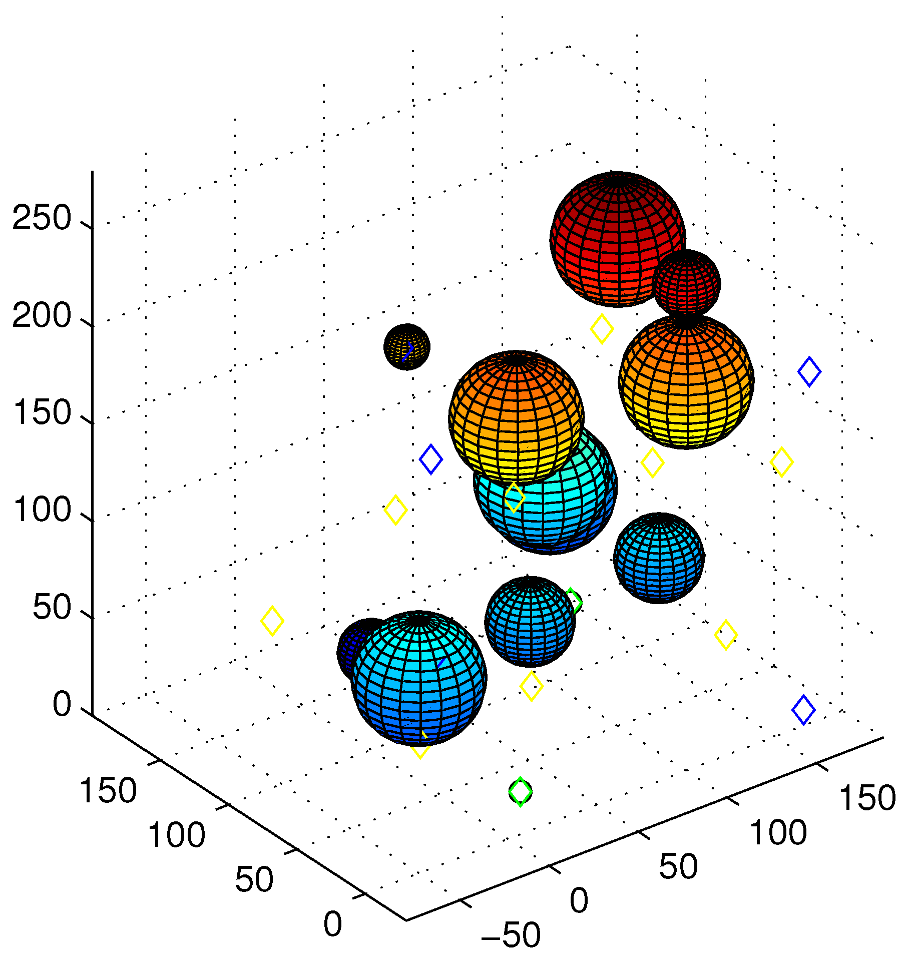
Figure 2 shows the final sensor configuration after the robots are deployed to cover the 3D workspace with a known size in meters. 966 s are spent to cover the workspace completely. Using MATLAB simulations, 7 s are spent to build the complete network without sensing holes. Among 50 robots, 18 robots move to cover the workspace. Yellow diamonds indicate robot positions dropped from , and blue diamonds indicate robot positions dropped from . The position of a ship is marked with a circle. In the figure, spheres indicate obstacles in the environment.
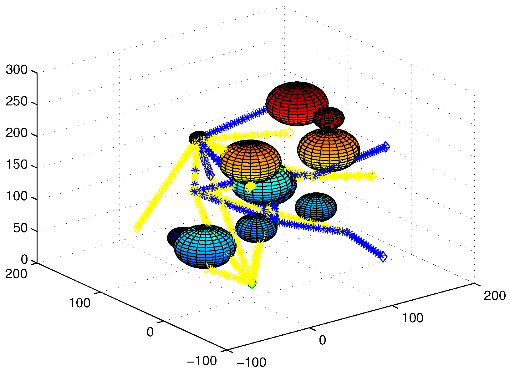
Considering the scenario in Figure 2, Figure 3 shows the sensor network that is built utilizing our 3D coverage methods. In Figure 3, the path of a robot that is dropped from the ship at is marked with yellow asterisks. Also, the path of a robot that is dropped from the ship at is marked with blue asterisks.
4.1. Estimate the Number of Robots Required
Next, we address how to estimate the number of robots required for covering a 3D workspace, considering the case where an obstacle inside the workspace is not known a priori. To estimate the number of robots, we simulate Algorithm 1, while setting no obstacles in the environment. We set no obstacles in the simulation, since we estimate the number of robots, in the case where an obstacle inside the workspace is not known a priori.
Figure 4 shows the sensor configuration, as Algorithm 1 is used to simulate the robot maneuvers for covering the 3D workspace with a known size in meters. See that there is no obstacle in the simulated environment.
In Figure 4, the path of a robot that is dropped from the ship at is marked with yellow asterisks. Also, the path of a robot that is dropped from the ship at is marked with blue asterisks. Using MATLAB simulations, 14 s are spent to build the complete network without sensing holes.
32 robots are dropped in the simulations, and the position of a robot is depicted with a green circle in Figure 4. Using the simulation in the workspace without obstacles, we can estimate the number of required robots as 32.
5. Discussions
In Algorithm 1, a robot moves along a directed path to reach its target position. A robot, which can be an AUV with acceleration constraints, can follow the path using path following controls in [29,30,31,32]. As a robot moves along a path, it must avoid collision with moving obstacles, such as other vehicles or animals. Various reactive collision avoidance methods [35,36,37] can be integrated with the proposed path planner, so that a robot can avoid collision with abrupt obstacles.
6. Conclusions
As a method to build underwater sensor networks in a cluttered underwater environment, this article considers surface ships dropping robots into the sea. Multiple robots move autonomously to build 3D sensor networks, while avoiding collision with unknown obstacles. The 3D coverage algorithm works by deploying a single robot at a time to spread out networks, until the open space is fully covered. Moreover, this article discusses how to handle broken robots, as well as how to estimate the number of robots required, considering the case where an obstacle inside the workspace is not known a priori.
Utilizing MATLAB simulations, we demonstrate the effectiveness of the proposed network construction methods. As our future works, we will do experiments to verify the proposed methods utilizing real underwater robots.
Funding
This work was supported by the National Research Foundation of Korea (NRF) grant funded by the Korea government (MSIT) (No. 2019R1F1A1063151).
Conflicts of Interest
The author declares no conflict of interest.
References
- Akyildiz, I.; Su, W.; Sankarasubramaniam, Y.; Cayirci, E. A survey on sensor networks. IEEE Commun. Mag. 2002, 40, 102–114. [Google Scholar] [CrossRef] [Green Version]
- Batalin, M.A.; Sukhatme, G.S. Coverage, exploration and deployment by a mobile robot and communication network. IEEE Commun. Mag. 2004, 26, 181–196. [Google Scholar] [CrossRef]
- Felemban, E.; Shaikh, F.K.; Qureshi, U.M.; Sheikh, A.A.; Qaisar, S.B. Underwater Sensor Network Applications: A Comprehensive Survey. Int. J. Distrib. Sens. Netw. 2015, 11, 896832. [Google Scholar] [CrossRef] [Green Version]
- Smith, B.; Howard, A.; McNew, J.; Egerstedt, M. Multi-Robot Deployment and Coordination with Embedded Graph Grammars. Auton. Robot. 2009, 26, 79–98. [Google Scholar] [CrossRef]
- Cortés, J.; Martínez, S.; Karatas, T.; Bullo, F. Coverage control for mobile sensing networks. IEEE Trans. Robot. Autom. 2004, 20, 243–255. [Google Scholar] [CrossRef]
- Siligardi, L.; Panerati, J.; Kaufmann, M.; Minelli, M.; Ghedini, C.; Beltrame, G.; Sabattini, L. Robust Area Coverage with Connectivity Maintenance. In Proceedings of the 2019 International Conference on Robotics and Automation (ICRA), Montreal, QC, Canada, 20–24 May 2019; pp. 2202–2208. [Google Scholar]
- Stergiopoulos, Y.; Kantaros, Y.; Tzes, A. Connectivity-aware coordination of robotic networks for area coverage optimization. In Proceedings of the 2012 IEEE International Conference on Industrial Technology, Athens, Greece, 19–21 March 2012; pp. 31–35. [Google Scholar]
- Ramaithitima, R.; Whitzer, M.; Bhattacharya, S.; Kumar, V. Sensor coverage robot swarms using local sensing without metric information. In Proceedings of the 2015 IEEE International Conference on Robotics and Automation (ICRA), Seattle, WA, USA, 26–30 May 2015; pp. 3408–3415. [Google Scholar]
- Franchi, A.; Masone, C.; Grabe, V.; Ryll, M.; Bülthoff, H.H.; Giordano, P.R. Modeling and Control of UAV Bearing Formations with Bilateral High-level Steering. Int. J. Robot. Res. 2012, 31, 1504–1525. [Google Scholar] [CrossRef]
- Luo, S.; Kim, J.; Parasuraman, R.; Bae, J.H.; Matson, E.T.; Min, B.C. Multi-robot rendezvous based on bearing-aided hierarchical tracking of network topology. Ad Hoc Netw. 2019, 86, 131–143. [Google Scholar] [CrossRef]
- Dehnavi, S.M.; Ayati, M.; Zakerzadeh, M.R. Three dimensional target tracking via Underwater Acoustic Wireless Sensor Network. In Proceedings of the 2017 Artificial Intelligence and Robotics (IRANOPEN), Qazvin, Iran, 9 April 2017; pp. 153–157. [Google Scholar]
- Kim, J. Three-dimensional multi-robot control to chase a target while not being observed. Int. J. Adv. Robot. Syst. 2019, 16, 1729881419829667. [Google Scholar] [CrossRef]
- Kim, J. Cooperative Exploration and Protection of a Workspace Assisted by Information Networks. Ann. Math. Artif. Intell. 2014, 70, 203–220. [Google Scholar] [CrossRef]
- Kim, J. Capturing intruders based on Voronoi diagrams assisted by information networks. Int. J. Adv. Robot. Syst. 2017, 14, 1–8. [Google Scholar] [CrossRef]
- Kim, J.; Maxon, S.; Egerstedt, M.; Zhang, F. Intruder Capturing Game on a Topological Map Assisted by Information Networks. In Proceedings of the 2011 50th IEEE Conference on Decision and Control and European Control Conference, Orlando, FL, USA, 12–15 December 2011; pp. 6266–6271. [Google Scholar]
- Kim, J. Intruder capture algorithms considering visible intruders. Int. J. Adv. Robot. Syst. 2019, 16, 1729881419846739. [Google Scholar] [CrossRef]
- Spagnolo, G.S.; Cozzella, L.; Leccese, F. Underwater Optical Wireless Communications: Overview. Sensors 2020, 20, 2261. [Google Scholar] [CrossRef] [PubMed]
- Wu, T.C.; Chi, Y.C.; Wang, H.Y.; Tsai, C.T.; Lin, G.R. Blue Laser Diode Enables Underwater Communication at 12.4 Gbps. Sci. Rep. 2017, 7, 1–10. [Google Scholar]
- Liu, J.; Wang, Z.; Cui, J.H.; Zhou, S.; Yang, B. A Joint Time Synchronization and Localization Design for Mobile Underwater Sensor Networks. IEEE Trans. Mob. Comput. 2016, 15, 530–543. [Google Scholar] [CrossRef]
- Misra, S.; Ojha, T.; Mondal, A. Game-Theoretic Topology Control for Opportunistic Localization in Sparse Underwater Sensor Networks. IEEE Trans. Mob. Comput. 2015, 14, 990–1003. [Google Scholar] [CrossRef]
- Han, G.; Zhang, C.; Shu, L.; Rodrigues, J.J.P.C. Impacts of Deployment Strategies on Localization Performance in Underwater Acoustic Sensor Networks. IEEE Trans. Ind. Electron. 2015, 62, 1725–1733. [Google Scholar] [CrossRef]
- Jadbabaie, A.; Lin, J.; Morse, A.S. Coordination of groups of mobile autonomous agents using nearest neighbor rules. IEEE Trans. Autom. Control 2003, 48, 349–368. [Google Scholar]
- McNew, J.M.; Klavins, E. Locally interacting hybrid systems with embedded graph grammars. In Proceedings of the 45th IEEE Conference on Decision and Control, San Diego, CA, USA, 13–15 December 2006; pp. 6080–6087. [Google Scholar]
- Pompili, D.; Melodia, T.; Akyildiz, I.F. Three-dimensional and two-dimensional deployment analysis for underwater acoustic sensor networks. Ad Hoc Netw. 2009, 7, 778–790. [Google Scholar] [CrossRef]
- Lin, Y.; Ni, C.; Lei, N.; David Gu, X.; Gao, J. Robot Coverage Path planning for general surfaces using quadratic differentials. In Proceedings of the 2017 IEEE International Conference on Robotics and Automation (ICRA), Singapore, 29 May–3 June 2017; pp. 5005–5011. [Google Scholar]
- Galceran, E.; Carreras, M. Planning coverage paths on bathymetric maps for in-detail inspection of the ocean floor. In Proceedings of the 2013 IEEE International Conference on Robotics and Automation, Karlsruhe, Germany, 6–10 May 2013; pp. 4159–4164. [Google Scholar]
- Douglas, B.W. Introduction to Graph Theory, 2nd ed.; Prentice Hall: Chicago, IL, USA, 2001. [Google Scholar]
- Calado, P.; Gomes, R.; Nogueira, M.B.; Cardoso, J.; Teixeira, P.; Sujit, P.B.; Sousa, J.B. Obstacle avoidance using echo sounder sonar. In Proceedings of the OCEANS 2011 IEEE, Santander, Spain, 6–9 June 2011; pp. 1–6. [Google Scholar]
- Peng, Z.; Wang, J.; Wang, J. Constrained Control of Autonomous Underwater Vehicles Based on Command Optimization and Disturbance Estimation. IEEE Trans. Ind. Electron. 2019, 66, 3627–3635. [Google Scholar] [CrossRef]
- Peng, Z.; Wang, J.; Han, Q. Path-Following Control of Autonomous Underwater Vehicles Subject to Velocity and Input Constraints via Neurodynamic Optimization. IEEE Trans. Ind. Electron. 2019, 66, 8724–8732. [Google Scholar] [CrossRef]
- Shen, C.; Shi, Y.; Buckham, B. Path-Following Control of an AUV: A Multiobjective Model Predictive Control Approach. IEEE Trans. Control Syst. Technol. 2019, 27, 1334–1342. [Google Scholar] [CrossRef]
- Suarez Fernandez, R.A.; Parra, R.E.A.; Milosevic, Z.; Dominguez, S.; Rossi, C. Nonlinear Attitude Control of a Spherical Underwater Vehicle. Sensors 2019, 19, 1445. [Google Scholar] [CrossRef] [Green Version]
- Ji, M.; Egerstedt, M. Distributed Coordination Control of Multi-Agent Systems While Preserving Connectedness. IEEE Trans. Robot. 2007, 23, 693–703. [Google Scholar] [CrossRef]
- Kim, J.; Kim, S. Motion control of multiple autonomous ships to approach a target without being detected. Int. J. Adv. Robot. Syst. 2018, 15, 1–8. [Google Scholar] [CrossRef]
- Chakravarthy, A.; Ghose, D. Obstacle avoidance in a dynamic environment: A collision cone approach. IEEE Trans. Syst. Man Cybern. 1998, 28, 562–574. [Google Scholar] [CrossRef] [Green Version]
- Van den Berg, J.; Guy, S.J.; Lin, M.; Manocha, D. Reciprocal n-Body Collision Avoidance. Robot. Res. Springer Tracts Adv. Robot. 2011, 70, 3–19. [Google Scholar]
- Kim, J. Control laws to avoid collision with three dimensional obstacles using sensors. Ocean Eng. 2019, 172, 342–349. [Google Scholar] [CrossRef]
Figure 1.
heads towards . Red curves indicate obstacle boundaries, and the path of is illustrated with yellow line segments. The large dots indicate the robots which are already at their target positions. FrontierPoints are depicted as points on one robot’s .
Figure 1.
heads towards . Red curves indicate obstacle boundaries, and the path of is illustrated with yellow line segments. The large dots indicate the robots which are already at their target positions. FrontierPoints are depicted as points on one robot’s .

Figure 2.
The final sensor configuration after the robots are deployed to cover the 3D workspace. Among 50 robots, 18 robots move to cover the workspace. Yellow diamonds indicate robot positions dropped from , and blue diamonds indicate robot positions dropped from . The ship position is marked with a circle. Spheres indicate obstacles in the environment.

Figure 3.
Considering the scenario in Figure 2, this figure shows the sensor network that is built under our 3D coverage methods. The path of a robot that is dropped from the ship at is marked with yellow asterisks. Furthermore, the path of a robot that is dropped from the ship at is marked with blue asterisks.

Figure 4.
The sensor configuration after the robots are simulated to cover the 3D workspace without obstacles. 32 robots are dropped in total, and the position of a robot is depicted with a green circle. The path of a robot that is dropped from the ship at is marked with yellow asterisks. Also, the path of a robot that is dropped from the ship at is marked with blue asterisks. Using the simulation in the workspace without obstacles, we can estimate the number of required robots as 32.

Publisher’s Note: MDPI stays neutral with regard to jurisdictional claims in published maps and institutional affiliations. |
© 2021 by the author. Licensee MDPI, Basel, Switzerland. This article is an open access article distributed under the terms and conditions of the Creative Commons Attribution (CC BY) license (https://creativecommons.org/licenses/by/4.0/).
Share and Cite
MDPI and ACS Style
Kim, J. Constructing 3D Underwater Sensor Networks without Sensing Holes Utilizing Heterogeneous Underwater Robots. Appl. Sci. 2021, 11, 4293. https://0-doi-org.brum.beds.ac.uk/10.3390/app11094293
AMA Style
Kim J. Constructing 3D Underwater Sensor Networks without Sensing Holes Utilizing Heterogeneous Underwater Robots. Applied Sciences. 2021; 11(9):4293. https://0-doi-org.brum.beds.ac.uk/10.3390/app11094293
Chicago/Turabian StyleKim, Jonghoek. 2021. "Constructing 3D Underwater Sensor Networks without Sensing Holes Utilizing Heterogeneous Underwater Robots" Applied Sciences 11, no. 9: 4293. https://0-doi-org.brum.beds.ac.uk/10.3390/app11094293
Note that from the first issue of 2016, this journal uses article numbers instead of page numbers. See further details here.