Article

Optimal Integration of Photovoltaic Sources in Distribution Networks for Daily Energy Losses Minimization Using the Vortex Search Algorithm

by
Alejandra Paz-Rodríguez
1,
Juan Felipe Castro-Ordoñez
1,
Oscar Danilo Montoya
2,3,* and
Diego Armando Giral-Ramírez
4
1
Ingeniería Eléctrica, Universidad Distrital Francisco José de Caldas, Bogotá D.C. 11021, Colombia
2
Facultad de Ingeniería, Universidad Distrital Francisco José de Caldas, Bogotá D.C. 11021, Colombia
3
Laboratorio Inteligente de Energía, Universidad Tecnológica de Bolívar, Cartagena 131001, Colombia
4
Facultad Tecnológica, Universidad Distrital Francisco José de Caldas, Bogotá D.C. 11021, Colombia
*
Author to whom correspondence should be addressed.
Submission received: 20 April 2021 / Revised: 5 May 2021 / Accepted: 11 May 2021 / Published: 13 May 2021

Abstract

:
This paper deals with the optimal siting and sizing problem of photovoltaic (PV) generators in electrical distribution networks considering daily load and generation profiles. It proposes the discrete-continuous version of the vortex search algorithm (DCVSA) to locate and size the PV sources where the discrete part of the codification defines the nodes. Renewable generators are installed in these nodes, and the continuous section determines their optimal sizes. In addition, through the successive approximation power flow method, the objective function of the optimization model is obtained. This objective function is related to the minimization of the daily energy losses. This method allows determining the power losses in each period for each renewable generation input provided by the DCVSA (i.e., location and sizing of the PV sources). Numerical validations in the IEEE 33- and IEEE 69-bus systems demonstrate that: (i) the proposed DCVSA finds the optimal global solution for both test feeders when the location and size of the PV generators are explored, considering the peak load scenario. (ii) In the case of the daily operative scenario, the total reduction of energy losses for both test feeders are 23.3643% and 24.3863%, respectively; and (iii) the DCVSA presents a better numerical performance regarding the objective function value when compared with the BONMIN solver in the GAMS software, which demonstrates the effectiveness and robustness of the proposed master-slave optimization algorithm.

1. Introduction

Electric power systems are composed of four sectors: generation, transmission/sub-transmission, distribution, and commercialization; the transmission and distribution networks are in charge of connecting the generation and consumption points over hundreds or thousands of kilometers [1]. In general, electric power transmission and distribution networks differ in the voltage levels at which they operate, which implies transmission voltages greater than 220 kV, between 57 and 220 kV for sub-transmission, and less than 57 kV for distribution [2]. However, the predominant voltage energy distribution level in Colombia ranges between 11.4 and 13.8 kV, respectively [3]. These electric networks present differences in their characteristics since the transmission usually uses meshed systems, and the distribution uses radial characteristics [4,5]. Due to these differences in electrical energy losses, the transmission levels are between 1.5% and 2% of the energy generated in peak hours, while the energy distribution can vary between 6% and 18%. The above-mentioned implies that, in the worst case, 18% of the distribution level energy is transformed into heat in the resistance lines and transformers in the distribution mainly [3,6]. Given the high levels of losses in the energy distribution, it is necessary to quantify them to determine an optimal solution to this problem [7].
There are different methods to reduce losses; for example, by reconfiguring the network using the binary gravitational search algorithm based on the algebraic graph theory [8]. Other examples include, through energy storage systems [9], and using particle swarm meta-heuristic optimization and genetic algorithms, with the inclusion of a static distribution compensator D-STATCOM that provides reactive power [7], and through the location and optimal size of distributed generation [8].
This article aims to reduce losses in distribution networks using the localization and the optimal size of PV systems, i.e., PV generators, in distribution systems with 33 and 69 nodes [6,10]. For this analysis, the generators inject active power according to their typical behavior during hours of solar radiation. Furthermore, the characteristic demand curve of the distribution networks is presented in this study. Due to the growing interest in solar energy for its benefits to the clear contribution of the trimming of CO2, in recent years, there has been an increase in research regarding this renewable energy, which focuses on issues associated with optimization, performance, and solar systems cells, among others, as mentioned in [11]. It means that the field of application of solar energy includes a wide variety of energy solutions, such as carrying out studies to reduce power and energy losses that integrate energy sources of renewable generation. For this, it is of vital importance to resort to metaheuristic techniques through algorithms. These algorithms use advantages that vary according to the implemented numerical optimization methods, which are adaptable algorithms to any problem. This variety allows finding a space solution that reduces losses [12] and costs of the distributed generation [13], which is because the algorithm provides the information necessary to determine the optimal solution.
The study of losses is a complex mixed integer nonlinear programming problem (MINLP). The MINLP structure of the optimization problem complicates the possibility of finding a globally optimal solution due to the non-convex shape of the solution space [14]. Therefore, a hybrid discrete-continuous modification of the vortex search algorithm (DCVSA) is proposed as a solution. So, it is necessary to use the unconventional method known as successive approximations (SA) [15] to evaluate the power flow problem. The DCVSA algorithm works through an optimization strategy that consists of a master stage responsible for determining the optimal location and size of the PV systems. In the same way, it considers that the location part belongs to the discrete segment and the size belongs to the continuous section, and a slave stage constantly evaluates the flow of energy through SA.
In short, carrying out a detailed review of the specialized literature, it was evident that, so far, there is no modification of the DCVSA to reduce energy losses based on the location and optimal size of the PV systems, which represents a research opportunity for this article. In this sense, Table 1 presents the information related to some of the methods recently used to reduce energy losses in distribution systems from 2012 to 2021.
From now on, the organization of the document is the following. Section 2 presents the problem formulation corresponding to the mathematical model, which involves the respective equation of the objective function and the restrictions. Section 3 explains and operates the solution methodology and its discrete-continuous hybrid coding and, additionally, presents the electrical parameters of the case studies (33 and 69 node systems), the demand loops, and the generation of a PV system. In Section 4, the reader can find a review and validation of the DCVSA algorithm concerning the specialized literature; the results obtained reducing energy losses are shown and compared. Section 5 presents the main conclusions and possible future works derived from this research, followed by acknowledgments and references.

2. MINLP Model

The integration of PV systems with the optimal location and dimensioning in distribution systems is a problem of the MINLP [14]. In the MINLP, the objective function is responsible for minimizing energy losses considering restrictions such as the power balance in the system, limits voltage at the nodes, characteristic demand curve, and generation limits of a PV system in 24 h. The MINLP model, as recommended in [6], will be developed in the complex domain for the sake of simplicity concerning the optimization approach that uses the DCVSA algorithm.

2.1. Objective Function

The objective function considered in this work corresponds to the minimization of energy losses in all the lines for the study period, which Equation (1) represents.
min E loss = r e a l i ϵ N j ϵ N h ϵ H Y i h Y i j V j h * Δ h
where E loss represents the energy losses, V i h is the bus voltage i in time h, V j h is the complex voltage for bus j in period h, Y i j is the complex admittance matrix that links the nodes i and j. It is necessary to clarify that N is the set that contains all the nodes of the system, H is the set that holds all the evaluated periods, and ( . ) * is the complex conjugate operator.

2.2. Restrictions

The optimal location problem and sizing of PV systems to minimize energy losses must accomplish different restrictions. Equation (2) describes the power balance that occurs in the distribution system.
S i h s + S i h p v S i h d = V i h j ϵ N Y i j V j h * , i , j ϵ N & h ϵ H
where S i h s is the complex power of the slack node connected to bus i in period h, S i h p v is the complex power of the PV system connected to bus i in period h, and S i h d is the complex power node demanded i in the term time h.
The second restriction corresponds to the voltage of each one of the system’s nodes and is described by Equation (3).
V min V i h V max , i ϵ N & h ϵ H
where V min and V max represent the lower and upper voltage bounds for each system node in different periods.
The third restriction refers to the generation capacity of a PV system and is described by Equation (4).
z i P min p v P i p v z i P max p v , i ϵ N
where
z i ϵ 0 , 1 , i ϵ N
z i describes the binary variable of the problem associated with the location of the PV systems; if z i = 1 , this represents the installation of a PV system in node i. Otherwise, z i = 0 , P min p v and P max p v are the minimum and maximum active power limits that a PV system can inject, and P i p v is the active power injected by a system PV in node i. It considers that the PV systems will only have an active power injection; therefore, for this model Q i p v = 0 [14].
Finally, Equation (6) describes the maximum number of PV systems set up in the distribution system.
i ϵ N z i N p v
where N p v is the maximum number of PV systems to install.
The MINLP model proposed for this case study allows evaluating the effect of active power injection in reducing energy losses through PV systems considering 24 h where both the demand and the generation of a system PV change hour by hour. However, due to the complexity of the MINLP model, it is necessary to use meta-heuristic optimization techniques [32], such as the DCVSA algorithm, which the next section details.

3. Materials and Methods

In this section, the proposed solution methodology is presented, which considers a master-slave strategy, where a DCVSA version of the algorithm is used in the master stage, which is in charge of defining the location and optimal size of the PV systems. In the slave stage, SA uses a multi-period power flow method responsible for solving the power flow equations for the generation data of a PV system assigned in the master stage. It, thus, determines energy losses for the study period. Below, each phase of the methodology is presented.

3.1. Vortex Search Algorithm (VSA)

The VSA is a solution based on a meta-heuristic approach that allows optimization of problems such as MINLP, whose operating principle is based on the search for vortices that adaptively change in size. It has two stages; the explorer stage is in charge of looking for a solution space, and the exploiting phase is in a load of evaluating the answers to find the optimal one within the solution space.
This algorithm can model through hyper-ellipses enclosed one after another; the first solution space of the explorer stage defines a hyper-ellipse whose center is the first answer to the problem [33]. For the case under study, the dimension proposed is six; since it establishes a maximum of three possible PV systems, whose vectors must contain three different locations. These locations correspond to the nodes where the PV system localizes and three sizes according to their capacity. x min and x max represent the minimal and maximum value of the vector and are value between 2 and N, with N being the maximum number of nodes in the network, where the minimum and maximum value of the PV system capacity is given between 0 and 2000 kW, as stated in [6]. Therefore, Equation (7) helps to find the center of the hyper-ellipse.
μ 0 = x 1 min + x 1 max 2 , x 2 min + x 2 max 2 , x 3 min + x 3 max 2 , x 4 min + x 4 max 2 , x 5 min + x 5 max 2 , x 6 min + x 6 max 2
Furthermore, it has a set of neighboring solutions C i t ( x ) where i corresponds to the position of the potential solution and t represents the current iteration of the algorithm, which initializes at 0. Said solutions within the solution space, defined by dimension six, are randomly generated using a Gaussian distribution, represented by Equation (8).
C i t ( x ) = p x | μ , Σ = 1 2 π d | Σ | e x p 1 2 x μ T Σ 1 x μ
where d represents the dimension, x is the solution vector d × 1 of a random value, μ is the vector d × 1 of the sample mean, and Σ is the covariance matrix. If the value of the diagonal elements of Σ are equal and those outside the diagonal are zero, then the resulting shape of the distribution will be a hyper-ellipse; therefore, the value of Σ can be calculated using equal variances with zero covariance, as presented in Equation (9).
Σ = σ 2 · [ I ] d × d
where σ represents the variance of the distribution, and I represents the identity matrix of dimension d × d . Equation (10) calculates the initial standard departure σ 0 of the distribution.
σ 0 = max x 1 max , x 2 max , x 3 max , x 4 max , x 5 max , x 6 max min x 1 min , x 2 min , x 3 min , x 4 min , x 5 min , x 6 min 2
where σ 0 is also considered the initial radius r 0 of the outer hyper ellipse, that is, the first solution space [34]. As a first step, by multiplying the initial radius by Equation (12), this solution space is expanded to obtain complete coverage.
The set of neighboring solutions obtained and contained in C i t ( x ) , verified within the algorithm and taking into account the lower and upper limits set in μ 0 , are defined by Equation (11).
C i t ( x ) = C i t ( x ) , x min x x max x min + x max x min r a n d , otherwise
where r a n d is a function that generates a random number between 1 and 0 with a normal distribution; after it verifies the limits, at this point, the exploiter stage comes into operation. It selects the most optimal response within the solution space of C i t obtained in (11) so that it is the new center μ of the hyper-ellipsoid [35].
Subsequently, in the hyper-ellipsoid, the effective radius is reduced to r t , so it must readjust the new radio to suit the process of searching for neighboring solutions through the inverse incomplete gamma function during each iteration. Equation (12) represents the incomplete gamma function.
Γ a = 0 x e t t a 1 · d t + x e t t a 1 · d t , a > 0 , x 0
In MATLAB, g a m m a i n c i n v ( g i n i v ) is the inverse incomplete gamma function, which computes the opposite of the incomplete gamma function concerning the integration limit x as g a m m a i n c i n v ( x , a ) . For the case under study, x = 0.1 and a ϵ [ 0 , 1 ] where Equation (13) explains a.
a = t r t max
where t max is the maximum number of iterations, and t r is a number that initializes equal to the maximum number of iterations but decreases by one unit as the iteration concludes. On the other hand, it is defined that t max can vary depending on the size of the system, which implies that the variation of a will change in the steps determined by t max . According to the above, Equation (14) defines the new radius of the new hyper-ellipsoid.
r t = 1 x · g a m m a i n c i n v ( x , a ) · x max x min 2
From the new radius r t [36], a new set of solutions is generated stored in C i t ( x ) , which implies that the value of the ensemble of neighboring solutions will be closer and closer as the radius decreases by each iteration.
Finally, the process of calculating the new radius, new center, and new solution spaces will successively repeat until it accomplishes one out of two termination conditions; if it reaches the maximum number of proposed iterations t max or if, after some consecutive iterations τ , it reaches the maximum number of sequential iterations τ m a x in which the center of the hyper-ellipsoid remains constant.

3.2. Hybrid Discrete-Continuous Vortex Search Algorithm (DCVSA) Encoding

The case study proposed in this article implemented a DCVSA version, where the structure of Equation (15) sets a solution space.
C i t = n , 2 , . . . , k | P min p v , P max p v , . . . , q
where i corresponds to the position of the potential solution and t to the current iteration. Furthermore, k represents a number of a random node, n the number of the last node in the system, and q a random number between P min p v and P max p v .
The candidate solutions of the solution space are divided into two parts. The first part represents the discrete variables of the problem since they are the nodes that can install the PV systems, while the second part depicts the continuous variables since they are the generation capacity that PV systems may have.
According to the above, and considering the restrictions of the MINLP model, the DCVSA algorithm will work as follows:
In its slave stage, the algorithm will solve the power flow from the SA method to identify the energy losses described in Equation (16). Figure 1 presents the solution diagram for the power flow problem using the SA method.
E l o s s = r e a l i ϵ N j ϵ N h ϵ H V i h Y i j V j h * Δ h
In its master stage, with hybrid coding, DCVSA will explore and exploit the solution space to identify the optimal location and dimensioning to reduce energy losses. Algorithm 1 represents the computational logic to implement the DCVSA based on the structure proposed in [7].
Algorithm 1: Implementation of the DCVSA algorithm for the optimal location and dimensioning of PV systems in distribution networks.
Applsci 11 04418 i001

3.3. Case Studies: Distribution Systems

The problem of optimal location and sizing of PV systems to reduce energy losses was raised and validated in the 33-node system, shown in Figure 2, and in the 69-node system, shown in Figure 3. These figures show the radial configuration of the distribution systems, whose base parameters are V b a s e = 12.66 kV and S b a s e = 1000 kVA taken at the slack node. For each one, the installation of three PV systems with a capacity of 0–2000 kW was considered.
The electrical parameters of connection between active and reactive power nodes, resistance, and reactance of the systems are shown [14]. Likewise, it is necessary to mention that these systems are urban distributions that feed industrial users as they have a single main generator that supplies a demand of 3.715 MW and 2.300 MVAr at peak hours in the 33-node system and 3.802 MW and 2.694 MVAr in the method of 69 nodes.
Table 2 demonstrates the variation in active power that a PV system can inject and the characteristic demand for the study proposed in this article.
According to Table 2, the pick load scenario occurs at hour 19, while the PV system will have variable generation from 8:00 a.m. to 7:00 p.m. The data of the percentage of consumption and energy availability for the PV system can be found in [14].

4. Results

The results of the cases under study were obtained for the optimal location and dimensioning of PV systems. They consider the behavior of a PV system and the characteristic demand of the systems for the reduction of energy losses. The DCVSA algorithm was modified and implemented with the SA method to solve the power flow. These results were obtained from MATLAB software, in version 2020b, the validation of which was executed on a PC with an Intel (R) Core (TM) i7-7700 CPU @ 3.60 GHz processor and memory 32.0 GB installed RAM running on a version of Windows 10 Pro.

4.1. Reduction of Power Losses in Peak Hours

Taking into consideration that the specialized literature reports the power losses for the peak hour, hour 19, Table 3 and Table 4 present the results for the study cases informed by the different methods, including the proposed DCVSA method.

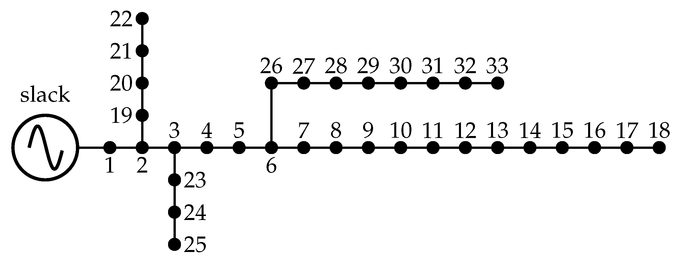
4.1.1. Distribution System of 33 Nodes

For the 33-node system, when there is no type of generation by a PV system, the power loss at the rush hour is 210.9876 kW. Considering the inclusion of three PV systems that inject active power into the system for this value, the power loss reduction is quantified for each method, as shown in Table 3. The value of power losses is directly affected by the location and capacity of each of the PV systems. The power demanded in the nodes where the PV systems are installed decreases thanks to the renewable generation provided; thus, the maximum loss reduction can be found through optimization techniques.
From the results obtained from the numerical validation carried out with the methods presented in Table 3, it states that:
The best method for solving the power loss reduction problem through the location and optimal generation size is MOHTLBOGWO, whose solution is the discrete vector of 13 , 24 , 30 as the location at the node of the generation and 0.9960 , 0.9380 , 0.8520 MW of installed capacity for a reduction in percentage losses of 65.8226%.
The results obtained by the DCVSA demonstrate the effectiveness of the proposed algorithm since it achieves the reduction of losses of the CBGA-VSA and DSCA-SOCP methods with a solution vector of nodes 13 , 24 , 30 and installed power of 0.8018 , 1.0913 , 1.0536 MW to achieve a percentage reduction of 65.5026% in power losses.
The DCVSA method proposed in this document presents a reduction in power losses of 65.5026% for the peak hour, with a total injection of the active power of 2.9476 MW. This result obtains a higher reduction in power losses than 86% of the methods presented in Table 3.
The power loss reduction of the proposed algorithm concerning the lower power loss reduction presented by HSA is higher by 29.8144%. Likewise, it represents that the DCVSA power loss reduction is 0.32% lower than the method with the highest power loss reduction presented by MOHTLBOGWO.

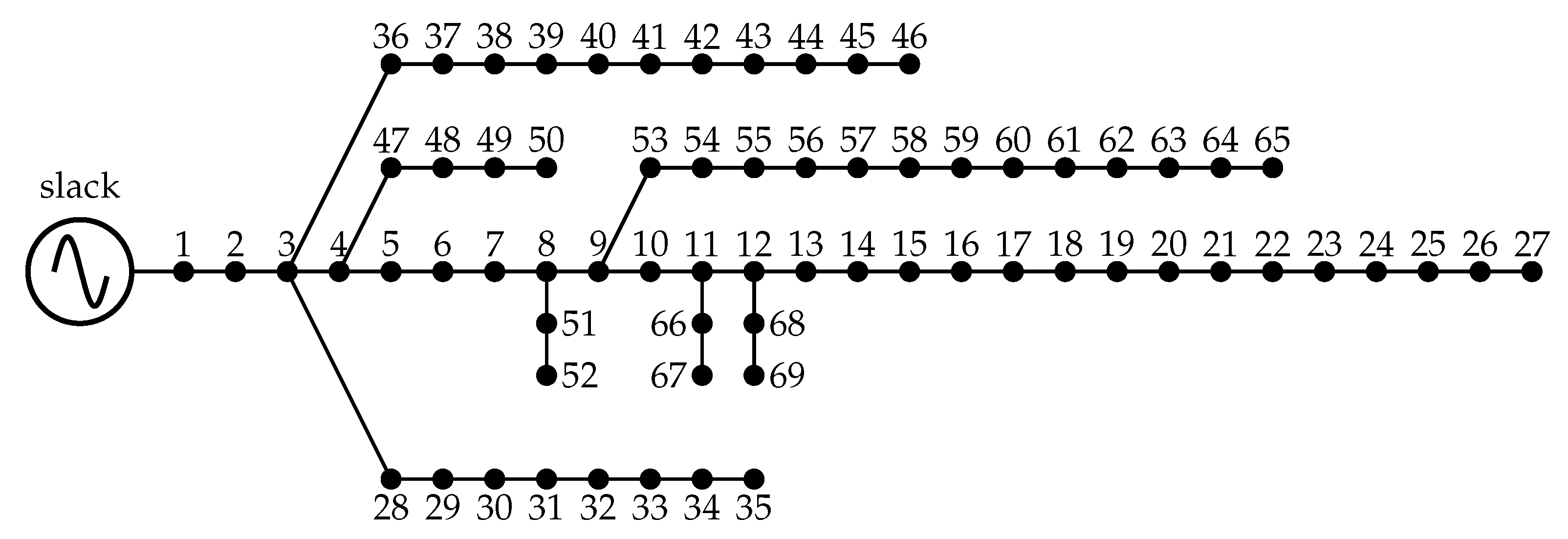
4.1.2. Distribution System of 69 Nodes

In the 69-node system, when there is no type of generation by a PV system, the power losses at peak hour are 224.9519 kW. Through this power, it is possible to quantify the reduction in power losses of each of the methods reported by the specialized literature, as shown in Table 4.
The results of the numerical validation shown in Table 4 state that:
Unlike the 33-node system, there are four methods among the most efficient for reducing power losses, with a location vector of 11 , 18 , 61 , of which one is the method proposed in this article. The reduction percentage of the power, the MSSA, DCVSA, CBGA-VSA, and DSCA-SOCP methods present 69.1455%, with the difference that the first proposes a total of 2.624 MW of installed power for the PV systems, while the three other systems rise to 2.6259 MW.
The DCVSA method proposed in this article presents a reduction in power losses for the peak hour of 69.1455% with a power injection in the nodes 11 , 18 , 61 of 0.5268 , 0.3801 , 1.7190 MW. This result presents a higher reduction in power losses than 84% of the methods represented in the comparative Table 4.
It validates the performance of the proposed algorithm concerning the presented lower reduction in power losses, which, unlike the 33-node system, is not HSA but PMC, which implies that the DCVSA is 9.8654% better.

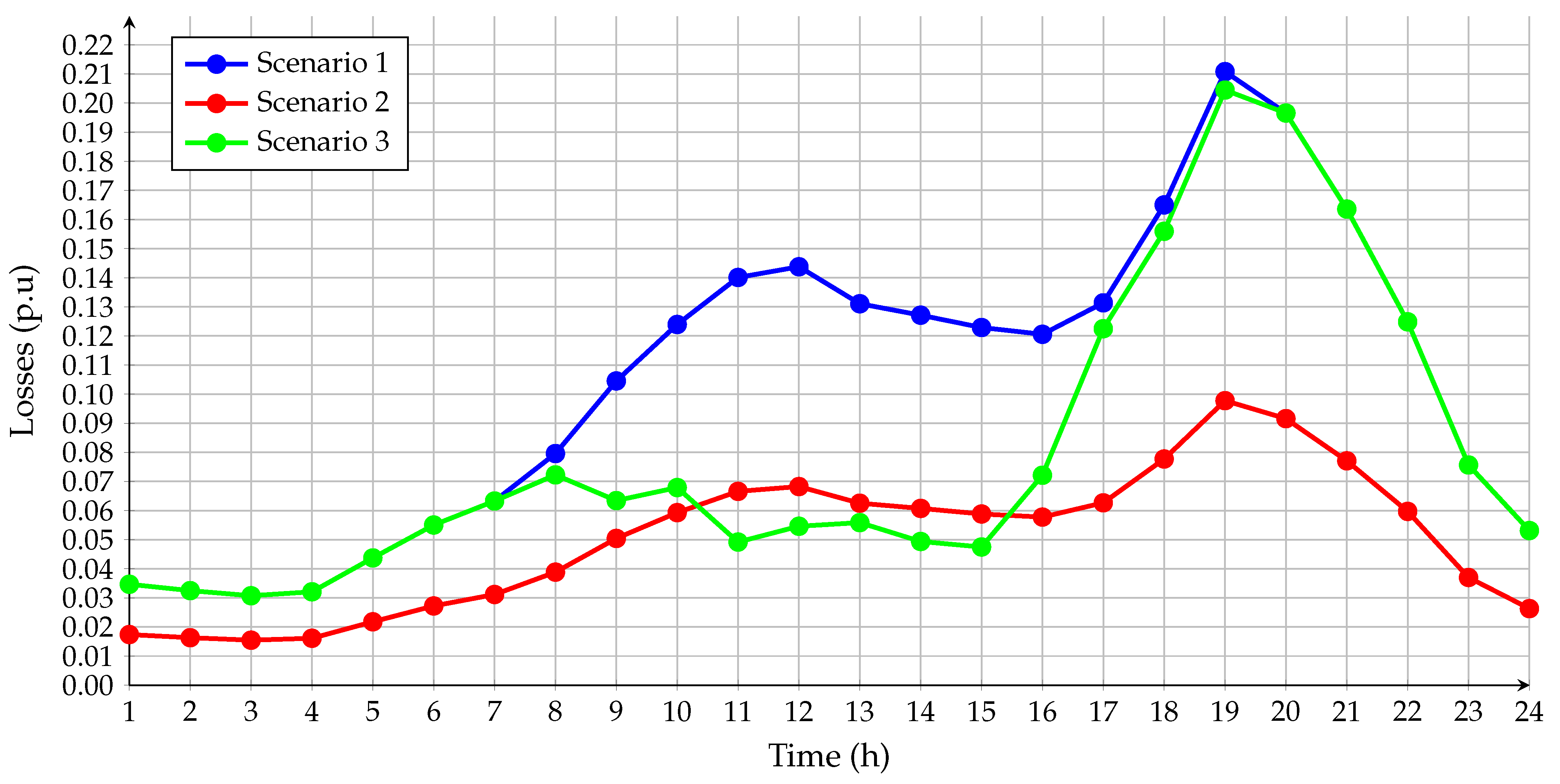
4.2. Reduction of Energy Losses for 24 h

Once the MINLP model and the DCVSA solution method proposed in this article are validated, the results of the energy loss reduction are analyzed for 24 h. Table 2 shows the characteristic demand curve and the variation in the generation of the PV system. In that sense, for the 33-node and 69-node systems, three scenarios are proposed in Table 5.
As shown in Table 5, the first scenario evaluates energy losses when there is no generation from a PV system. The second scenario considers a constant PV system of 1 p.u during 24 h. The third scenario is the closest to reality, as it poses a variable PV system with the characteristic curve of energy availability presented in Table 2.

4.2.1. Distribution System of 33 Nodes

Figure 4 shows the results obtained for the scenarios set out in Table 5, in this test system, with a solution vector in terms of location of 14 , 24 , 30 and sizing of 1.1332 , 1.5824 , 1.5531 MW. In the hours in which there is active power generation (7:00–20:00) by the PV systems, it shows a reduction in energy losses, while in the hours where there is no injection of active power (1:00–7:00 and 20:00–24:00), scenario (3) is similar to the behavior obtained in scenario (1).
On the other hand, from 11:00–15:00, scenario (3) presents a higher reduction in energy losses than scenario (2). It indicates that for that period, the most beneficial thing is not to inject 100% of the capacity of the PV systems; therefore, there must be a balance between the energy generated and the demand. If this balance does not occur, the PV systems will contribute energy losses through the electric current injected into the system by I 2 R .
Table 6 shows the results of the energy losses for the three scenarios proposed in the 33-node system. These results were obtained through the sum of the power losses for each hour of the day. With the DCVSA algorithm, when considering the up-and-down behavior of the PV systems concerning scenario (1), a reduction in energy losses of 23.3643% was obtained. It is also possible to analyze that scenario (2) has a decrease of energy losses of 52.1867 % regarding scenario (1); however, this result is hypothetical since the production availability of PV systems is not ideal and only considers those hours where there is solar radiation.

4.2.2. Distribution System of 69 Nodes

Figure 5 shows the results obtained for the scenarios set out in Table 5, in this test system, with a solution vector in terms of location of 17 , 61 , 64 and sizing of 0.7735 , 2.0000 , 0.5835 MW. It displays that, as in the 33-node system, in the hours in which there is active power generation (7:00–20:00) by the PV systems, there is a reduction in energy losses. Meanwhile, in the hours where there is no active power injection generated (1:00–7:00 and 20:00–24:00), scenario (3) has similar behavior scenario (1).
On the other hand, as in the 33-node system, from 11:00–15:00, scenario (3) presents a higher reduction in energy losses than scenario (2). Due to searching for the optimal energy reduction vector, it may be oversized for those hours since the capacity of the PV system changed according to the demand hour by hour. This may not be beneficial because the losses could increase beyond expected— not as the demand increased but as a surplus generation.
Table 7 shows the results of energy losses for the three scenarios proposed. With the DCVSA algorithm, a reduction in energy losses of 24.3863% was obtained when considering the up-and-down behavior of the PV systems concerning scenario (1). It is also possible to analyze that scenario (2) had a reduction in energy losses of 54.8861 % regarding scenario (1); however, this result is hypothetical because, as mentioned above, the production availability of PV systems is not ideal.

4.2.3. Comparative Analysis for Reducing Energy Losses with GAMS

To validate the reduction of energy losses proposed in scenario (3) and the proposed algorithm, a comparative analysis using the GAMS software and its BONMIN solver was carried out to solve the exact mathematical model given by Equations (1)–(6) [37]. According to the above, for the systems of 33 and 69 nodes, Table 8 and Table 9 present the solution vectors of the PV systems results obtained for scenario (3) with the GAMS-BONMIN method and the DCVSA method proposed in this article.
From Table 8, it is evident that, for the 33-node system, the GAMS-BONMIN method presents a percentage of reduction of energy losses of 18.8808% concerning scenario (1), which shows it is inferior to the proposed method. The DCVSA represents an efficiency increase of 4.4835% since the solution vector considers 14 , 24 , 30 as the nodes to install the PV systems and 1.1332 , 1.5824 , 1.5531 MW as their installed capacity.
On the other hand, in Table 9, the comparison of the two methods can be observed again, but this time for the system of 69 nodes, where the GAMS-BONMIN method with the proposed solution vector achieves a reduction in energy losses of 23.0151%. For this system, DCVSA obtains a reduction in energy losses 1.3712% greater than the GAMS-BONMIN method. The difference in the decrease of energy losses for the 69-node system is not that wide since the location of the PV systems is very similar; only node 5 for GAMS-BONMIN changes to node 17 for DCVSA, and the difference in installed power is 0.286 MW higher for the DCVSA method.

4.3. Additional Comments

The results of Section 4.2, for the 33-node system, were obtained after running the DCVSA algorithm with an average response of 1679.1267 seconds. Likewise, in this test system, the average response time was 4771.6179 seconds. The maximum difference in energy losses was 12.4286 kWh/day considering the characteristic demand curve and the generation variation of a PV system for both networks. This maximum difference can improve by increasing the sampling and the number of iterations for the DCVSA; since for systems, such as the 69-node, and those with more branches, having a higher number of variables results in a slower convergence.
Regarding the response of the solution vectors for the 33-node system to reduce power and energy losses, it states that the location for reducing power losses was 13 , 24 , 30 . In the same way, it denotes that the position for decreasing energy losses was 14 , 24 , 30 , where the total installed power for PV systems is 2.9467 MW and 4.2687 MW, respectively. This means that the overall installed capacity required to reduce energy losses over a period of 24 h cannot be measured only taking into account the peak hour since an increase of 30.9686% is necessary concerning the total required during the 24 h.
Likewise, in the 69-node system, it is outstanding to mention that the location nodes of the PV systems were different for the power and energy cases since in the first, it was 11 , 18 , 61 , and in the second, it was 17 , 61 , 64 . On the other hand, it displays that the capacity of the installed power to reduce losses in hour 19 was 2.6258 MW. Furthermore, for the decrease of energy losses, it was 3.3569 MW, which indicates that the installation of PV systems considering 24 hours a day should increase by 21.7785%.

5. Conclusions

The injection of the maximum capacity of PV systems is not an optimal solution for reducing losses in distribution systems. On the contrary, under some scenarios, wastes may present an increase. Thus, it is necessary to propose optimization strategies that allow the decrease of losses, the optimal location, and the measurement of PV systems. This study addresses the loss reduction problem by implementing the MINLP model and the DCVSA meta-heuristic solution method.
As input, first, the demand curve and the PV generation available for 24 h were characterized. This analysis considered the drop of power losses for the peak hour and the decrease of power losses for the total period. The peak hour analysis evidences the efficacy of the DCVSA method developed concerning the specialized literature. The assay of energy losses for the overall period proves the effectiveness of the DCVSA method developed for GAMS-BONMIN.
The proposed DCVSA algorithm reduced power losses by 65.5% and 69.15% for 33-node and 69-node systems. From the analysis of energy losses, DCVSA reduced them by 23.36% and 24.39% for the 33-node and 69-node systems, respectively. The execution times and the maximum difference in energy losses presented in the simulations denote the effectiveness and accuracy of the DCVSA and the proposed MINLP model.
Finally, regarding this article, future studies can be derived, such as: (i) the inclusion of other systems that provide renewable energy to distribution networks (i.e., wind and geothermal generation), (ii) broadening of the application of methods for reducing power losses, including energy storage systems, focused on energy studies, and (iii) changing the proposed MINLP mathematical model to obtain a convex equivalent that guarantees a unique solution.

Author Contributions

Conceptualization, A.P.-R.; J.F.C.-O.; O.D.M.; and D.A.G.-R.; methodology, A.P.-R.; J.F.C.-O.; O.D.M.; and D.A.G.-R.; investigation, A.P.-R.; J.F.C.-O.; and O.D.M.; writing—review and editing, A.P.-R.; J.F.C.-O.; O.D.M.; and D.A.G.-R. All authors have read and agreed to the published version of the manuscript.

Funding

This research received no external funding.

Institutional Review Board Statement

Not applicable.

Informed Consent Statement

Not applicable.

Data Availability Statement

No new data were created or analyzed in this study. Data sharing is not applicable to this article.

Acknowledgments

This work has been derived from the undergraduate project:“Integración óptima de fuentes fotovoltaicas en sistemas de distribución para disminuir las pérdidas diarias de energía empleando el algoritmo de optimización de búsqueda por vórtices” presented by the students Alejandra Paz Rodríguez and Juan Felipe Castro Ordoñez to the Electrical Engineering Program of the Engineering Faculty at Universidad Distrital Francisco José de Caldas as a partial requirement for the Bachelor in Electrical Engineering.

Conflicts of Interest

The authors declare no conflict of interest.

Nomenclature

Other Symbols
eEuler number.
i,jIndices of nodes in the system.
tCurrent iteration of the algorithm.
t r The maximum number of iterations decreasing by one for each iteration t.
Mathematical Operators
· * Complex conjugate operator.
· T Transpose matrix operator.
· 1 Inverse matrix operator.
Γ Incomplete gamma function.
D d Diagonal of the conjugate matrix V d (V).
g i n i v Inverse incomplete gamma function in MATLAB.
I d × d Identity matrix of dimension d × d .
r a n d Function for a random number between 1 and 0 with normal distribution.
Parameters
ϵ Maximum error of the successive approximations method.
S i h d Complex power demanded at the node i in period h (VA).
S i h p v Complex power of the PV system connected to the bus i in period h (VA).
S i h s Complex power of the slack node connected to the bus i in period h (VA).
μ 0 Initial center of the hyper-ellipsoid.
σ 0 Initial standard deviation of the Gaussian distribution.
τ m a x Maximum number of continued iterations with the center of the hyper-ellipsoid constant.
HSet containing all evaluated periods.
NSet that contains all the nodes of the system.
t max The maximum number of iterations.
dDimension of the solution space.
N p v The highest PV systems install number.
P max p v The PV system maximum active power (W).
P min p v The PV system minimal active power (W).
r 0 Initial radius of the hyper-ellipse.
S b a s e Base power for the case studies (VA).
S d Complex power of the demand nodes (VA).
V max System nodes maximum voltage value (V).
V min System nodes minimal voltage value (V).
V b a s e Base voltage for the case studies (V).
V g Voltage value of the generation nodes (V).
Variables
V i h Bar voltage i in period h (V).
V j h Bar voltage j in period h (V).
Y The matrix admittance that relates the nodes of the system (S).
Y d d Component of the matrix admittance that relates the demand nodes among them (S).
Y d g Component of the matrix admittance that relates the demand nodes with generation nodes (S).
Y i j Complex admittance matrix that relates nodes i and j (S).
Z d d Component of the matrix impedance that relates the demand nodes among them ( Ω ).
μ Vector of dimension d × 1 of the sample mean.
Σ Covariance matrix.
σ Variance of the Gaussian distribution.
τ Number of consecutive iterations.
E loss Value of energy losses in the study period (Wh/day).
kNumber of a random node.
mCounter of the successive approximations method.
qRandom power between P min p v and P max p v (W).
C i t Gaussian distribution for solutions with position i and iteration t.
I d Current value of the demand nodes (A).
P i p v Active power injected by a PV system at node i (W).
r t Radius at iteration t.
V d Voltage value of the demand nodes (V).
xSolution vector of dimension d × 1 of a random value.
x max Maximum amount of the solution vector.
x min Minimum amount of the solution vector.
z i Existence of a PV system at node i.

References

  1. UPME. Reference Expansion Planning Generacion Transmision 2004–2018; Resreport, Unidad de Planeación Minero Energética: Bogotá, Colombia, 2004. [Google Scholar]
  2. Castro-Galeano, J.C.; Cabra-Sarmiento, W.J.; Ortiz-Portilla, J.F. Fault and load flows analysis of electricity transmission and distribution system in Casanare (Colombia). Rev. Fac. Ing. 2017, 26, 7. [Google Scholar] [CrossRef] [Green Version]
  3. Montoya, O.D.; Serra, F.M.; Angelo, C.H.D. On the Efficiency in Electrical Networks with AC and DC Operation Technologies: A Comparative Study at the Distribution Stage. Electronics 2020, 9, 1352. [Google Scholar] [CrossRef]
  4. Grisales-Noreña, L.; Montoya, D.G.; Ramos-Paja, C. Optimal Sizing and Location of Distributed Generators Based on PBIL and PSO Techniques. Energies 2018, 11, 1018. [Google Scholar] [CrossRef] [Green Version]
  5. Montoya, O.D.; Gil-González, W.; Orozco-Henao, C. Vortex search and Chu-Beasley genetic algorithms for optimal location and sizing of distributed generators in distribution networks: A novel hybrid approach. Eng. Sci. Technol. Int. J. 2020, 23, 1351–1363. [Google Scholar] [CrossRef]
  6. Montoya, O.D.; Molina-Cabrera, A.; Chamorro, H.R.; Alvarado-Barrios, L.; Rivas-Trujillo, E. A Hybrid Approach Based on SOCP and the Discrete Version of the SCA for Optimal Placement and Sizing DGs in AC Distribution Networks. Electronics 2020, 10, 26. [Google Scholar] [CrossRef]
  7. Montoya, O.D.; Gil-González, W.; Hernández, J.C. Efficient Operative Cost Reduction in Distribution Grids Considering the Optimal Placement and Sizing of D-STATCOMs Using a Discrete-Continuous VSA. Appl. Sci. 2021, 11, 2175. [Google Scholar] [CrossRef]
  8. Esmaeilian, H.; Fadaeinedjad, R.; Attari, S. Distribution network reconfiguration to reduce losses and enhance reliability using binary gravitational search algorithm. In Proceedings of the 22nd International Conference and Exhibition on Electricity Distribution (CIRED 2013), Stockholm, Sweden, 10–13 June 2013. [Google Scholar]
  9. Krstic, N. Reduction of Energy and Power Losses in Distribution Network Using Energy Storage Systems. In Proceedings of the 2020 55th International Scientific Conference on Information, Communication and Energy Systems and Technologies (ICEST), Niš, Serbia, 10–12 September 2020. [Google Scholar]
  10. Kaur, S.; Kumbhar, G.; Sharma, J. A MINLP technique for optimal placement of multiple DG units in distribution systems. Int. J. Electr. Power Energy Syst. 2014, 63, 609–617. [Google Scholar] [CrossRef]
  11. Reyes-Belmonte, M.A. Quo Vadis Solar Energy Research? Appl. Sci. 2021, 11, 3015. [Google Scholar] [CrossRef]
  12. Catalbas, M.C.; Gulten, A. Circular structures of puffer fish: A new metaheuristic optimization algorithm. In Proceedings of the 2018 Third International Conference on Electrical and Biomedical Engineering, Clean Energy and Green Computing (EBECEGC), Beirut, Lebanon, 24–26 April 2018. [Google Scholar]
  13. Samala, R.K.; Kotapuri, M.R. Hybridization of Metaheuristic Algorithms for Optimal Location and Capacity in Radial Distribution System. In Proceedings of the 2019 2nd International Conference on Power and Embedded Drive Control (ICPEDC), Chennai, India, 21–23 August 2019. [Google Scholar]
  14. Montoya, O.D.; Gil-González, W.; Grisales-Noreña, L. An exact MINLP model for optimal location and sizing of DGs in distribution networks: A general algebraic modeling system approach. Ain Shams Eng. J. 2020, 11, 409–418. [Google Scholar] [CrossRef]
  15. Montoya, O.D.; Gil-González, W. On the numerical analysis based on successive approximations for power flow problems in AC distribution systems. Electr. Power Syst. Res. 2020, 187, 106454. [Google Scholar] [CrossRef]
  16. Moradi, M.; Abedini, M. A combination of genetic algorithm and particle swarm optimization for optimal DG location and sizing in distribution systems. Int. J. Electr. Power Energy Syst. 2012, 34, 66–74. [Google Scholar] [CrossRef]
  17. Injeti, S.K.; Kumar, N.P. A novel approach to identify optimal access point and capacity of multiple DGs in a small, medium and large scale radial distribution systems. Int. J. Electr. Power Energy Syst. 2013, 45, 142–151. [Google Scholar] [CrossRef]
  18. Mohanty, B.; Tripathy, S. A teaching learning based optimization technique for optimal location and size of DG in distribution network. J. Electr. Syst. Inf. Technol. 2016, 3, 33–44. [Google Scholar] [CrossRef] [Green Version]
  19. Kollu, R.; Rayapudi, S.R.; Sadhu, V.L.N. A novel method for optimal placement of distributed generation in distribution systems using HSDO. Int. Trans. Electr. Energy Syst. 2012, 24, 547–561. [Google Scholar] [CrossRef]
  20. Sultana, S.; Roy, P.K. Multi-objective quasi-oppositional teaching learning based optimization for optimal location of distributed generator in radial distribution systems. Int. J. Electr. Power Energy Syst. 2014, 63, 534–545. [Google Scholar] [CrossRef]
  21. Muthukumar, K.; Jayalalitha, S. Optimal placement and sizing of distributed generators and shunt capacitors for power loss minimization in radial distribution networks using hybrid heuristic search optimization technique. Int. J. Electr. Power Energy Syst. 2016, 78, 299–319. [Google Scholar] [CrossRef]
  22. Jamian, J.; Mustafa, M.; Mokhlis, H. Optimal multiple distributed generation output through rank evolutionary particle swarm optimization. Neurocomputing 2015, 152, 190–198. [Google Scholar] [CrossRef] [Green Version]
  23. Gupta, S.; Saxena, A.; Soni, B.P. Optimal Placement Strategy of Distributed Generators based on Radial Basis Function Neural Network in Distribution Networks. Procedia Comput. Sci. 2015, 57, 249–257. [Google Scholar] [CrossRef] [Green Version]
  24. Bayat, A.; Bagheri, A. Optimal active and reactive power allocation in distribution networks using a novel heuristic approach. Appl. Energy 2019, 233–234, 71–85. [Google Scholar] [CrossRef]
  25. Moradi, M.; Abedini, M. A novel method for optimal DG units capacity and location in Microgrids. Int. J. Electr. Power Energy Syst. 2016, 75, 236–244. [Google Scholar] [CrossRef]
  26. Sultana, S.; Roy, P.K. Krill herd algorithm for optimal location of distributed generator in radial distribution system. Appl. Soft Comput. 2016, 40, 391–404. [Google Scholar] [CrossRef]
  27. Nguyen, T.P.; Dieu, V.N.; Vasant, P. Symbiotic Organism Search Algorithm for Optimal Size and Siting of Distributed Generators in Distribution Systems. Int. J. Energy Optim. Eng. 2017, 6, 1–28. [Google Scholar] [CrossRef]
  28. Deshmukh, R.; Kalage, A. Optimal Placement and Sizing of Distributed Generator in Distribution System Using Artificial Bee Colony Algorithm. In Proceedings of the 2018 IEEE Global Conference on Wireless Computing and Networking (GCWCN), Lonavala, India, 23–24 November 2018. [Google Scholar]
  29. Nowdeh, S.A.; Davoudkhani, I.F.; Moghaddam, M.H.; Najmi, E.S.; Abdelaziz, A.; Ahmadi, A.; Razavi, S.; Gandoman, F. Fuzzy multi-objective placement of renewable energy sources in distribution system with objective of loss reduction and reliability improvement using a novel hybrid method. Appl. Soft Comput. 2019, 77, 761–779. [Google Scholar] [CrossRef]
  30. Gholami, K.; Parvaneh, M.H. A mutated salp swarm algorithm for optimum allocation of active and reactive power sources in radial distribution systems. Appl. Soft Comput. 2019, 85, 105833. [Google Scholar] [CrossRef]
  31. Bocanegra, S.Y.; Montoya, O.D. Heuristic approach for optimal location and sizing of distributed generators in AC distribution networks. WSEAS Trans. Power Syst. 2019, 14, 113–121. [Google Scholar]
  32. HassanzadehFard, H.; Jalilian, A. A novel objective function for optimal DG allocation in distribution systems using meta-heuristic algorithms. Int. J. Green Energy 2016, 13, 1615–1625. [Google Scholar] [CrossRef]
  33. Doğan, B.; Ölmez, T. A new metaheuristic for numerical function optimization: Vortex Search algorithm. Inf. Sci. 2015, 293, 125–145. [Google Scholar] [CrossRef]
  34. Gil-González, W.; Montoya, O.D.; Rajagopalan, A.; Grisales-Noreña, L.F.; Hernández, J.C. Optimal Selection and Location of Fixed-Step Capacitor Banks in Distribution Networks Using a Discrete Version of the Vortex Search Algorithm. Energies 2020, 13, 4914. [Google Scholar] [CrossRef]
  35. Doğan, B.; Ölmez, T. Vortex search algorithm for the analog active filter component selection problem. AEU Int. J. Electron. Commun. 2015, 69, 1243–1253. [Google Scholar] [CrossRef]
  36. Saka, M.; Tezcan, S.S.; Eke, I.; Taplamacioglu, M.C. Economic load dispatch using vortex search algorithm. In Proceedings of the 2017 4th International Conference on Electrical and Electronic Engineering (ICEEE), Ankara, Turkey, 8–10 April 2017. [Google Scholar]
  37. Soroudi, A. Power System Optimization Modeling in GAMS; Springer International Publishing: New York, NY, USA, 2017. [Google Scholar]
Figure 1. Flowchart of the proposed power flow method based on successive approximations.
Applsci 11 04418 g001
Figure 2. IEEE radial 33-node test system.
Applsci 11 04418 g002
Figure 3. IEEE radial 69-node test system.
Applsci 11 04418 g003
Figure 4. The behavior of power losses for each hour of the study period in the 33-node system.
Applsci 11 04418 g004
Figure 5. The behavior of power losses for each hour of the study period in the 69-node system.
Applsci 11 04418 g005
Table 1. Methods recently used to reduce energy losses in distribution systems.
AcronymOptimization MethodRef.Year
GAGenetic Algorithm[16]2012
PSOParticle Swarm Optimization[16]2012
LSFSALoss Sensitivity Factor Simulated Annealing[17]2013
TLBOTeaching Learning Based Optimization[18]2014
PMCParallel Monte Carlo[4]2014
HSAHarmony Search Algorithm[19]2014
QOTLBOQuasi-Oppositional Teaching Learning Based Optimization[20]2014
HSA-PABCHarmony Search Algorithm and Particle Artificial Bee Colony Algorithm[21]2014
MINLPMixed-Integer Nonlinear Programming Formulation[10]2014
REPSORank Evolutionary Particle Swarm Optimization[22]2015
RBFNN-PSORadial Basis Function Neural Network and Particle Swarm Optimization[23]2015
AHAAlgorithmic Heuristic Approach[24]2016
GA-IWDGenetic Algorithm and Intelligent Water Drops[25]2016
KHAKrill-Herd Algorithm[26]2016
SOSSymbiotic Organism Search[27]2017
PBIL-PSOPopulation-Based Incremental Learning and Particle Swarm Optimizer[4]2018
ABCAArtificial Bee Colony Algorithm[28]2018
MOHTLBOGWOMulti-Objective Hybrid Teaching–Learning Based Optimization-Grey Wolf Optimizer[29]2019
MSSAMutated Salp Swarm Algorithm[30]2019
CHVSAConstructive Heuristic Vortex Search Algorithm[31]2019
GAMSGeneral Algebraic Modeling System[14]2020
CBGA-VSAChu and Beasley Genetic Algorithm and Vortex Search Algorithm[5]2020
DSCA-SOCPDiscrete Sine Cosine Algorithm and Second-Order Cone Programming[6]2021
Table 2. Characteristic data of demand and generation of a PV system.
HourDemand (p.u)PV System Generation (p.u)HourDemand (p.u)PV System Generation (p.u)
10.42400130.80130.926
20.41080140.78990.851
30.39990150.77740.521
40.40830160.77740.255
50.47440170.80220.035
60.53010180.89260.028
70.566901910.015
80.63260.0490200.96820
90.72020.2490210.88900
100.78050.300220.78320
110.82680.683230.61750
120.83690.835240.52120
Table 3. Location and sizing of PV systems in the 33-node system.
Method P loss (kW)Nodes LocalizationSizing (MW)
MOHTLBOGWO72.1100 13 , 24 , 30 0.9960 , 0.9380 , 0.8520
CBGA-VSA72.7853 13 , 24 , 30 0.8018 , 1.0913 , 1.0536
DSCA-SOCP72.7853 13 , 24 , 30 0.8018 , 1.0913 , 1.0536
MSSA72.7854 13 , 24 , 30 0.8010 , 1.0910 , 1.0530
MINLP72.7862 13 , 24 , 30 0.8000 , 1.0900 , 1.0500
GAMS72.7900 14 , 24 , 30 0.7709 , 1.0969 , 1.0658
HSA-PABC72.8129 14 , 24 , 30 0.7550 , 1.0730 , 1.0680
AHA72.8340 13 , 24 , 30 0.7920 , 1.0680 , 1.0270
QOTLBO74.1008 12 , 24 , 29 0.8808 , 1.0592 , 1.0714
KHA75.4116 13 , 25 , 30 0.8107 , 0.8368 , 0.8410
REPSO76.9100 06 , 14 , 31 1.2274 , 0.6068 , 0.6870
CHVSA78.4534 06 , 14 , 31 1.1846 , 0.6468 , 0.6881
LSFSA82.0300 06 , 18 , 30 1.1124 , 0.4874 , 0.8679
PBIL-PSO91.5000 12 , 15 , 31 0.4035 , 0.5245 , 0.6422
PMC91.6000 12 , 18 , 31 0.4993 , 0.3966 , 0.6744
TLBO104.000 09 , 18 , 31 0.8847 , 0.8953 , 1.1958
SOS104.190 06 , 28 , 29 2.2066 , 0.2000 , 0.7167
PSO105.350 08 , 13 , 32 1.1768 , 0.9816 , 0.8297
GA106.300 11 , 29 , 30 1.5000 , 0.4228 , 1.0714
GA-IWD110.510 11 , 16 , 32 1.2214 , 0.6833 , 1.2135
HSA135.690 16 , 17 , 18 0.5927 , 0.2133 , 0.1913
DCVSA72.7853 13 , 24 , 30 0.8018 , 1.0913 , 1.0536
Table 4. Location and sizing of PV systems in the 69-node system.
Method P loss (kW)Nodes LocalizationSizing (MW)
MSSA69.4077 11 , 18 , 61 0.5260 , 0.3800 , 1.7180
CBGA-VSA69.4077 11 , 18 , 61 0.5268 , 0.3801 , 1.7190
DSCA-SOCP69.4077 11 , 18 , 61 0.5268 , 0.3801 , 1.7190
CHVSA69.4088 11 , 17 , 61 0.5284 , 0.3794 , 1.7186
MINLP69.4090 11 , 17 , 61 0.5300 , 0.3800 , 1.7200
KHA69.5730 12 , 22 , 61 0.4962 , 0.3113 , 1.7354
AHA69.6669 12 , 21 , 61 0.4710 , 0.3120 , 1.6890
QOTLBO71.6345 18 , 61 , 63 0.5334 , 1.1986 , 0.5672
MOHTLBOGWO71.7400 18 , 61 , 62 0.5230 , 1.0000 , 0.7730
GAMS72.0900 12 , 61 , 64 0.8131 , 1.4447 , 0.2896
LSFSA77.1000 18 , 60 , 65 0.4962 , 0.3113 , 1.7354
GA-IWD80.9100 20 , 61 , 64 0.9115 , 1.3926 , 0.8059
TLBO81.0000 25 , 60 , 63 0.7574 , 1.0188 , 1.1784
SOS82.0800 57 , 58 , 61 0.2588 , 0.2000 , 1.5247
PSO83.2000 17 , 61 , 63 0.9925 , 1.1998 , 0.7956
HSA86.6600 63 , 64 , 65 1.6283 , 0.1416 , 0.0149
PBIL-PSO86.9000 26 , 61 , 66 0.1789 , 1.0532 , 0.4209
GA89.0000 21 , 62 , 64 0.9297 , 1.0752 , 0.9925
PMC91.6000 63 , 68 , 69 1.2000 , 0.0577 , 0.3954
DCVSA69.4077 11 , 18 , 61 0.5268 , 0.3801 , 1.7190
Table 5. Scenarios to quantify the reduction of energy losses.
ScenarioCharacteristic
(1)Power losses without PV system
(2)Power losses with constant PV system
(3)Power losses with variable PV system
Table 6. Power losses for 33-node system scenarios.
Scenario E loss (kWh/day)
(1)2508.6343
(2)1199.4596
(3)1922.5098
Table 7. Power losses for 69-node system scenarios.
Scenario E loss (kWh/day)
(1)2664.7952
(2)1202.1918
(3)2014.9508
Table 8. Comparison of energy losses for the 33-node system.
MethodNodes LocalizationSizing (MW) E loss (kWh/day)
GAMS-BONMIN 08 , 24 , 25 1.9082 , 0.8805 , 0.4963 2034.9850
DCVSA 14 , 24 , 30 1.1332 , 1.5824 , 1.5531 1922.5098
Table 9. Comparison of energy losses for the the 69-node system.
MethodNodes LocalizationSizing (MW) E loss (kWh/day)
GAMS-BONMIN 05 , 61 , 64 0.8470 , 1.8750 , 0.3490 2051.4900
DCVSA 17 , 61 , 64 0.7735 , 2.0000 , 0.5835 2014.9508
Publisher’s Note: MDPI stays neutral with regard to jurisdictional claims in published maps and institutional affiliations.

