Revisiting Label Smoothing Regularization with Knowledge Distillation

Abstract

Label Smoothing Regularization (LSR) is a widely used tool to generalize classification models by replacing the one-hot ground truth with smoothed labels. Recent research on LSR has increasingly focused on the correlation between the LSR and Knowledge Distillation (KD), which transfers the knowledge from a teacher model to a lightweight student model by penalizing their output’s Kullback–Leibler-divergence. Based on this observation, a Teacher-free Knowledge Distillation (Tf-KD) method was proposed in previous work. Instead of a real teacher model, a handcrafted distribution similar to LSR was used to guide the student learning. Tf-KD is a promising substitute for LSR except for its hard-to-tune and model-dependent hyperparameters. This paper develops a new teacher-free framework LSR-OS-TC, which decomposes the Tf-KD method into two components: model Output Smoothing (OS) and Teacher Correction (TC). Firstly, the LSR-OS extends the LSR method to the KD regime and applies a softer temperature to the model output softmax layer. Output smoothing is critical for stabilizing the KD hyperparameters among different models. Secondly, in the TC part, a larger proportion is assigned to the uniform distribution teacher’s right class to provide a more informative teacher. The two-component method was evaluated exhaustively on the image (dataset CIFAR-100, CIFAR-10, and CINIC-10) and audio (dataset GTZAN) classification tasks. The results showed that LSR-OS can improve LSR performance independently with no extra computational cost, especially on several deep neural networks where LSR is ineffective. The further training boost by the TC component showed the effectiveness of our two-component strategy. Overall, LSR-OS-TC is a practical substitution of LSR that can be tuned on one model and directly applied to other models compared to the original Tf-KD method.

1. Introduction

Deep learning has been a story of booms of success; yet, as the network becomes deeper and wider, the model consumes more and more computational resources [1,2,3]. There is a trend to use light models with fewer parameters to save memory and accelerate learning and inferring speed [4,5,6,7]. With a carefully designed supernet space and model searching strategy, Neural Architecture Search (NAS) techniques [8,9] can find proper models to fit different requirements (flops, memory). Besides that, efforts are delivered to extract a small model from powerful large ones, e.g., pruning [10], binarization [11], encoding [12], and knowledge distillation [13].

As Figure 1a shows, KD [13] compresses the knowledge from the teacher model, which is a larger model or a set of multiple models, to a single small student model. Besides the traditional classification cross-entropy error (Figure 1b), a Kullback–Leibler (KL)-divergence loss is also penalized between a pre-trained teacher and the student model during the student training time. The KL-divergence is a measure of how two distributions are different from each other. By minimizing KL-divergence loss, a student model can mimic the inter-class relationship of the teacher prediction. Note that the softmax temperature ${\tau }_1$ for the KL-loss in KD is usually larger than one, which is the common choice of traditional cross-entropy loss (${\tau }_0$ = 1). In addition to its many application in model compression, KD is also used to boost network training with multiple models with an identical architecture [14,15] or a single-model self-distillation [16,17,18].

On the other hand, LSR was first proposed by Szegedy et al. [19] to regularize the Inception network on the ImageNet dataset. The traditional classification model calculates the cross-entropy loss between the model output and the one-hot ground truth vector, whereas LSR assigns a small ratio for the logits of the incorrect class and reduces the ratio of the ground truth class from one to a reasonably smaller value (Figure 1c). Since Szegedy et al. [19], LSR has been widely used in image classification [20,21,22], speech recognition [23], and machine translation [24].

Recently, plenty of research stressed the correlation of label smoothing regularization and knowledge distillation [25,26,27,28,29]. Reference [26] showed that LSR is equivalent to penalizing the KL-divergence between a uniform distribution and the model output distribution. Since KD penalizes the KL-divergence of the teacher and student distribution, this uniform distribution in LSR provides a virtual teacher model for KD [27] (Figure 1d). From a Maximum A Posterior (MAP) perspective, Reference [28] interpreted self-knowledge distillation as an instance-specific label smoothing regularization.

Based on the observation of the strong correlation between the KD method and LSR above, Yuan et al. [27] proposed the Teacher-free KD (Tf-KD) method that abandoned the traditional teacher model output. As Figure 1e shows, a manually designed teacher is used with a high proportion $\gamma$ on the correct class. Then, a high-temperature (${\tau }_2$≥ 20) softmax function is applied to smooth this teacher distribution. A different temperature ${\tau }_1$ is also applied to the student model output logits for the KL-loss. Tf-KD is a promising substitution of LSR and an effective alternative to KD methods without extra cost for teacher model training and forward propagation. However, the hyperparameters (temperature ${\tau }_1$, ${\tau }_2$ and proportion $\gamma$) in Tf-KD are model dependent and hard to tune. These shortcomings limit its wide use where LSR is applied conveniently.

The motivation of this work was to overcome the troublesome parameter-tuning issue of Tf-KD and provide a practical teacher-free method. Therefore, we proposed LSR-OS-TC, which improves the generalization of a model with two components: Output Smoothing (OS) and Teacher Correction (TC). We reformulated the LSR method in the KD expression. Instead of manually designing a teacher directly as Tf-KD, we first considered the importance of a softer temperature in KD [13]. The LSR method in KD form (Figure 1d) is generalized to LSR-OS (Figure 1f) by smoothing the model output with a hyperparameter temperature $\tau$ instead of one. Then, to make the uniform distribution teacher more informative, we proposed a Teacher Correction (TC) component for which a constant larger proportion $\gamma$ is assigned for the correct class in the uniform distribution. Unlike the manually designed teacher in Tf-KD, which needs a further hyperparameter ${\tau }_2$ to smooth, our designed distribution with TC is used directly as the teacher for the KL-loss. The TC component abandons the redundant hyperparameter ${\tau }_2$ in Tf-KD.

On the other hand, the traditional KD method stabilizes the gradient by multiplying a factor ${\tau }^2$ with the KL-loss. However, with the theoretical analysis of the KL-loss gradient of LSR-OS-TC, we argue that for a manually designed distribution with teacher correction, the KL-loss needs to be multiplied by $\tau$ instead. We believe this is the reason for the difficulty of Tf-KD parameter tuning.

The proposed methods were evaluated exhaustively on image classification datasets (CIFAR-100, CIFAR-10 [30], and CINIC-10 [31]) with various networks (ResNet [1], PreActResNet [32], and WideResNet (WRN) [33]). We also conducted LSR-OS-TC on a video dataset, GTZAN [34], for music genre classification. The results demonstrated that LSR has little improvement when the network is deep or complicated, whereas LSR-OS and its TC variant can consistently help train different network architectures. The independent effectiveness of LSR-OS and further improvement by TC indicate the effectiveness of our two-component decomposition.

The contributions of this work are summarized as follows:

• By extending label smoothing regularization in KD form with two separate components, LSR-OS-TC provides a reliable substitution to LSR. Specifically, Output Smoothing (OS) extends the LSR in KD form and applies a softer temperature to stabilize the learning. On the other hand, Teacher Correction (TC) assigns a larger proportion to the ground truth class to constitute a more informative teacher.
• Theoretically and experimentally, we analyzed the gradient of KL-loss in the LSR-OS-TC method and offered two tips that are critical for the training performance: multiplying $\tau$ instead of ${\tau }^2$ with the KL-loss and using a lower temperature.
• The experimental results demonstrate that the proposed method LSR-OS-TC outperforms the original LSR and the previous teacher-free method. Overall, LSR-OS-TC is a practical substitution of LSR that can be tuned on one model and directly applied to other models.

2. Related Work

2.1. Multiple Model KD for Boost Training

The Born-Again Network (BAN) [14] trained students parameterized identically to their teacher and outperformed their teachers significantly. The authors used the pre-trained model as a teacher to train a student and set the trained student as the teacher for the next training iteration. However, the recurrent distillation of BAN requires high computation and storage costs.

The deep mutual learning method [15] adopted an ensemble of students to learn collaboratively and showed that the mutual learning strategy performs better than the static teacher–student mode. Furthermore, a larger teacher net can also benefit from this mutual learning. However, aggregating students’ logits to form an ensemble teacher restrains student peers’ diversity, thus limiting the effectiveness of online learning [35]. Their work showed an essential characteristic of KD: the teacher is not necessarily perfect nor accurate. An intermediate teacher that matches the student’s training procedure is comparable to a thoroughly pre-trained teacher [36].

2.2. Single Model KD

Reference [16] proposed a self-distillation method that divides a single network into several sections connected with additional bottlenecks and fully connected layers to constitute multiple classifiers. Then, the knowledge in the deepest classifier of the network is squeezed into the shallower ones. The study of self-distillation is promising; they claimed that the teacher branch improves the shallower sections’ learning features. Luan et al. [37] deepened the shallower section’s bottleneck classifier and applied mutual learning distillation instead of the teacher–student method and achieved better performance. This improvement of MSD indicates that the self-distillation method can be regarded as a DML method of four peers with different low-level weight sharing. We evaluated four-model DML directly and found comparable results. Except with fewer parameters, this self-distillation method [16] can also be regarded as a multi-model KD method as DML. These network remodeling or model ensembling methods [16,38,39] have the limitation of generalization and flexibility.

Furthermore, KD-loss can also regularize the model output consistency of similar training samples, such as augmented data and original data [18], or samples that belong to the same classes [17]. However, the former method relies on the augmentation method’s efficacy, and the latter needs a carefully designed training procedure.

2.3. Label Smoothing with KD

The traditional classification tasks always utilize a one-hot vector as the target. The converged model is prone to over-fitting to the ground-truth label, i.e., a large difference between the largest logit and others. The label smoothing regularization method [19] assigns a small ratio for the incorrect class logits and reduces the ground truth ratio class from one to a reasonably smaller value. Yuan et al. [27] showed the equivalence of LSR and the KL-divergence penalization between a uniform distribution and the model output distribution. It is well known that the uniform distribution has the largest entropy. Thus, LSR will penalize low entropy outputs that are over-confident about the predictions. Visualization of the penultimate layer’s activation [40] shows that LSR makes the representations of the same class training examples closer to each other.

Reference [27] found that KD can be interpreted as a regularization method, and they revealed the relation between KD and LSR. Their proposed Teacher-free KD (Tf-KD) method abandoned the traditional teacher, which was always a model output. They first manually designed the teacher with a high proportion $\gamma$ on the correct class and then applied a high temperature ($\tau$≥ 20) on the KD-loss. The hyperparameters in Tf-KD are model dependent and hard to tune. Our LSR-OS method emphasizes that a proper soft temperature is more critical than the hand-crafted teacher. LSR-OS-TC was tuned on one model and performed consistently on all models. Without conducting the LSR in KD form, Reference [25] helped the training on CIFAR-100 by replacing the uniform distribution in the LSR method directly with the output of a teacher model pre-trained on the ImageNet dataset.

3. Preliminaries

3.1. Label Smoothing Regularization

We considered a standard classification problem. Given a training dataset D = {(x${}^i$, y${}^i$)}${}_{i=1}^N$, where x${}^i$ is the i${}_{th}$ sample from M classes and y${}^i$∈ {1, 2,..., M} is the corresponding label of sample x${}^i$, the parameters $\theta$ of a deep neural network (DNN) that best fit the dataset need to be determined.

The softmax function is employed to calculate the mth class probability from a given model:

$$p_m\left(\tau \right)=\frac{exp(z_m/\tau )}{{\sum }_{i=1}^{M}exp(z_i/\tau )}.$$

(1)

Here, z${}_m$ is the m${}_{th}$ logit output of the model’s fully connected layer. $\tau$ indicates the temperature of the softmax distribution normally set to one in traditional cross-entropy loss, but greater than one in knowledge distillation loss [13]. A larger $\tau$ means a softer probability distribution that reveals more detail than a hard softmax output ($\tau$ = 1).

For M-class classification, the traditional cross-entropy loss of a sample is as follows:

$$L_{CE}(p\left(1\right),q)=-\sum _{m=1}^M{q}_{m}log\left(p_m\left(1\right)\right),$$

(2)

where q${}_m$ is the m${}_{th}$ element of one-hot label vector q. Note that the temperature $\tau$ is set to one. The pipeline is depicted in Figure 1b.

For a training example with one-hot label vector q, the label smoothing regularization method (Figure 1c) [19] replaces q as q${}^{\prime }$:

$$q^{\prime }=(1-\alpha )\times q+\alpha \times u,$$

(3)

where u is a uniform distribution. Then, the cross-entropy loss of LSR is:

$$L_{LSR}(p\left(1\right),q^{\prime })=-\sum _{m=1}^M{q}_m^{\prime }log\left(p_m\left(1\right)\right),$$

(4)

Compared to the traditional cross-entropy loss, minimizing the loss between the model output and smoothed label q${}^{\prime }$ can help the model generalize better on the validation dataset.

3.2. Knowledge Distillation

As Figure 1a shows, a large teacher network is usually trained beforehand in the traditional knowledge distillation method. Then, to transfer the knowledge from the pre-trained teacher model to the student, the Kullback–Leibler (KL)-divergence between their output probabilities is penalized:

$$L_{KL}(p^t\left(\tau \right)\left|\right|p\left(\tau \right))=\sum _{m=1}^M{p}_m^t\left(\tau \right)log(\frac{p_m^t\left(\tau \right)}{p_m\left(\tau \right)}),$$

(5)

where $p^t\left(\tau \right)$ and $p\left(\tau \right)$ are the soft teacher and student distribution obtained from their corresponding model output with Equation (1). The temperature $\tau$ (>1) is a hyperparameter that needs to be tuned. During training, the KD method calculates the sum of the two losses above with a hyperparameter $\alpha$:

$$L_{KD}=(1-\alpha )\times L_{CE}(p\left(1\right),q)+\alpha \times {\tau }^2\times L_{KL}(p^t\left(\tau \right)\left|\right|p\left(\tau \right)),$$

(6)

where ${\tau }^2$ is a factor in ensuring that the relative contribution of the ground-truth label and teacher output distribution remains roughly unchanged [13].

3.3. Teacher-Free Knowledge Distillation

The cross-entropy loss in Equation (4) of LSR can be written as a KD-loss, similar to Equation (6):

$$\begin{array}{cc}\hfill L_{LSR}(p,q)& =L_{CE}(p\left(1\right),q^{\prime })\hfill \\ \hfill & =(1-\alpha )\times L_{CE}(p\left(1\right),q)+\alpha \times L_{KL}\left(u\right|\left|p\left(1\right)\right),\hfill \end{array}$$

(7)

which means that LSR can be regarded as a special case of KD with a uniform distribution teacher and $\tau$ = 1. Based on the above observation, Yuan et al. [27] proposed the Teacher-free Knowledge Distillation (Tf-KD) (Figure 1e) with the following loss function:

$$L_{Tf-KD}(p,q)=(1-\alpha )\times L_{CE}(p\left(1\right),q)+\alpha \times {\tau }^2\times multiplier\times L_{KL}(p^{\prime }\left({\tau }_1\right)\left|\right|p\left({\tau }_2\right)).$$

(8)

where ${\tau }_1$ and ${\tau }_2$ are different hyperparameters. The uniform distribution teacher u in Equation (7) is substituted as below [27]:

$$p_m^{\prime }=\left\{\begin{array}{cc}\gamma ,\hfill & m=c\hfill \\ \frac{1-\gamma }{M-1},\hfill & m\ne c\hfill \end{array}\right.$$

(9)

where c is the correct class and $\gamma$ is the probability of class c. Therefore, a 100% correct teacher is obtained by combining a uniform distribution and the ground truth label information.

Tf-KD is a promising substitution of LSR and an effective alternative of KD methods without extra cost for teacher model training and forward propagation. However, the Tf-KD method may suffer from the multiple hyperparameters: $\alpha$, multiplier, $\gamma$, ${\tau }_1$, and ${\tau }_2$. For different networks, the optimal parameter set may change dramatically. The proportion of two losses needs to be tuned by two parameters ($\alpha$ and multiplier) to guarantee the performance. These troublesome parameter tunings of Tf-KD may cost more computational resources to tune than other traditional KD methods with external knowledge. This disadvantage makes Tf-KD less attractive to researchers.

4. Method

Equation (7) shows the equivalence of LSR and KD. The Tf-KD method utilizes this equivalence mechanically to replace the uniform distribution teacher and many hyperparameters in Equation (8). To extend LSR in KD form more reasonably, we proposed the LSR-OS-TC method, which decomposes Tf-KD into two components organically. We proposed the LSR-OS component (Section 4.1) and amend it with the teacher correction in Section 4.2. Finally, the KL-loss gradient with the influence of temperature $\tau$ is theoretically analyzed in Section 4.3.

4.1. Component 1: Output Smoothing

Reference [13] showed that a soft temperature larger than one is critical for the effectiveness of KD, so we extended the KL-loss to a generalized form and put forward the LSR-OS component:

$$L_{LSR-OS}(p,q)=(1-\alpha )\times L_{CE}(p\left(1\right),q)+\alpha \times {\tau }^2\times L_{KL}\left(u\right|\left|p\left(\tau \right)\right).$$

(10)

The temperature $\tau$ is a critical factor in knowledge distillation methods. Increasing the temperature $\tau$ for the model output in Equation (8) generates a smoother probability distribution. An example of a model prediction is shown in Figure 2a; the predicted class is C8, which has the largest probability portion. The prediction $p_m\left(\tau \right)$ corresponding to the ${\mathit{m}}_{th}$ class is calculated by Equation (1). With $\tau$ increasing, the predicted class value is decreased, and the remaining classes obtain a greater share. The smoothed model output distribution reduces the large confidence values and reveals more details of the smaller ones. It is reasonable to minimize the KL-loss between the uniform distribution teacher and the model output smoothed with a flexibly adjusted temperature than a hard output ($\tau$ = 1) in the original LSR method.

4.2. Component 2: Teacher Correction

Similar to Tf-KD, a manually designed teacher with the true label information can help LSR-OS further. The uniform distribution teacher can be replaced by p${}^{\prime }$. In this paper, the replacement of the uniform distribution is named the teacher correction component. Then, we rewrite the LSR-OS loss with teacher correction as follows:

$$L_{LSR-OS-TC}(p,q)=(1-\alpha )\times L_{CE}(p\left(1\right),q)+\alpha \times \tau \times L_{KL}\left(p\left(\tau \right)\right||p^{\prime }).$$

(11)

As Figure 1g shows, the manually designed teacher soft target of LSR-OS-TC is a smoothing distribution with the correct class information.

The loss function of LSR-OS-TC omits the temperature parameter for the teacher distribution since the teacher distribution is already manually designed. The softmax in Equation (1) is usually applied to the model’s logits output for a model prediction, which is a distribution that indicates the probability for each class. Thus, it is not reasonable to apply a softmax function to the manually designed teacher just for a smoother teacher. A smoother teacher can be obtained by tuning the $\gamma$ in Equation (9) directly. On the other hand, LSR-OS-TC does not need a multiplier or the portion of KL-loss to stabilize different networks. The KL-loss gradient stabilizing factor ${\tau }^2$ in Equation (6) switches to $\tau$. The reason is explained in Section 3.3.

Overall, a simplified version of Tf-KD is proposed: LSR-OS-KD. With a thorough search of the hyperparameters ($\alpha$, multiplier, $\gamma$, ${\tau }_1$, and ${\tau }_2$), Tf-KD may reach similar performance as LSR-OS-TC. However, this fussy parameter searching will make the theoretically convenience of the teacher-free method meaningless. LSR-OS-TC retains the computational benefit of Tf-KD and removes the redundancy settings.

4.3. Gradient Analyses

In the KD method, a factor ${\tau }^2$ on the KL-loss is applied to stabilize the back-prop gradient while $\tau$ is changing. Here, we analyze the KL-loss gradient with $\tau$ in Equation (8) briefly, similar to [13]:

$$\begin{array}{cc}\hfill \frac{\partial L_{KL}(p\left(\tau \right),u)}{\partial z_m}& =\frac{1}{\tau }(p_m\left(\tau \right)-u_m)\hfill \\ \hfill & =\frac{1}{\tau }(\frac{exp(z_m/\tau )}{{\sum }_{i=1}^{M}exp(z_i/\tau )}-u_m).\hfill \end{array}$$

(12)

If the temperature is high with respect to the logits’ magnitude and the logits of the model output have been zero-meaned, Equation (11) simplifies to:

$$\begin{array}{cc}\hfill \frac{\partial L_{KL}(p\left(\tau \right),u)}{\partial z_m}& \approx \frac{1}{\tau }(\frac{1+z_m/\tau }{M}-u_m)\hfill \\ \hfill & =\frac{1}{M\tau }(z_m/\tau -(M{u}_m-1))\hfill \\ \hfill & =\frac{z_m}{M{\tau }^2}.\hfill \end{array}$$

(13)

From the above, the LSR-OS stage penalizes large and confidence logit values [26] in the high-temperature limit. Since the gradient of the KL-loss is scaled by 1/${\tau }^2$, it is necessary to multiply the KL-loss by ${\tau }^2$ to ensure the relative contribution of the two losses (Equation (8)). As Figure 2b shows, the KL-loss drops dramatically with the temperature $\tau$ growing. However, after ${\tau }^2$ is multiplied, the KL-loss is stabilized to a roughly similar magnitude (Figure 2c).

The reader may notice that we used a different temperature value for the second term in Equations (8) and (10). This is because the gradient of LSR-OS with teacher correction acts differently:

$$\begin{array}{cc}\hfill \frac{\partial L_{KL}(p\left(\tau \right),p^{\prime })}{\partial z_m}& =\frac{1}{\tau }(p_m\left(\tau \right)-p_m^{\prime })\hfill \\ \hfill & =\frac{1}{\tau }(\frac{exp(z_m/\tau )}{{\sum }_{i=1}^{M}exp(z_i/\tau )}-p_m^{\prime }).\hfill \end{array}$$

(14)

Similarly, with the high temperature and zero-meaned logit output assumption, Equation (13) simplifies to:

$$\begin{array}{cc}\hfill \frac{\partial L_{KL}(p\left(\tau \right),p^{\prime })}{\partial z_m}& \approx \frac{1}{\tau }(\frac{1+z_m/\tau }{M}-p_m^{\prime })\hfill \\ \hfill & =\frac{1}{M\tau }(z_m/\tau -(M{p}_m^{\prime }-1))\hfill \\ \hfill & =\frac{1/M-p_m^{\prime }}{\tau }.\hfill \end{array}$$

(15)

Note that M$p_m^{\prime }$ − 1 is a non-zero constant. The result of Equation (14) gives us two inferences:

• First, to stabilize the learning of LSR-OS-TC, we need to multiply a factor $\tau$ with the KL-loss term (Equation (10)) instead of ${\tau }^2$, which is the traditional choice of knowledge distillation methods (Equation (6)).
• Second, with an excessively high temperature, the logit loses the participation in the KL-loss gradient. In this case, the KL-loss gradient becomes constant and inoperative. A relatively small temperature $\tau$ is a more reasonable choice.

5. Experiments

In this section, we conducted experiments to evaluate LSR-OS-TC on four datasets for image and audio classification: CIFAR100 [41], CIFAR10 [41], CINIC10 [31], and GTZAN [34]. We focused our experiments on the CIFAR-100 dataset with the most networks and training details. CIFAR-10 and CINIC-10 are ten-class tasks that are easier; thus, the performance differences among different network results are small. Thus, we picked four networks that have a larger performance gap. The GTZAN dataset is a music genre classification task that is different from traditional image recognition. Due to the difference between the STFT spectrogram and a regular image, the frequently used CNN networks like ResNet cannot obtain satisfactory results. The networks nnet1 and nnet2 from Zhang et al. [42] were used as the baseline to evaluate the methods.

For a fair comparison, all results on the same dataset were obtained with the same setting. We implemented the networks and training procedures in PyTorch and conducted all experiments on a single NVIDIA TITAN RTX GPU.

The baseline results are the corresponding networks trained with the regular cross-entropy loss. Besides LSR-OS-TC and the baseline, we also provide the results of LSR [19] and the Tf-KD method. Tf-KD was proposed by Yuan et al. [27], which first manually-designed a teacher distribution and then applied a high temperature ($\tau$≥ 20) on KD-loss. Note that the hyperparameters in Tf-KD are model dependent and hard to tune. We proceeded with several runs to determine the temperature $\tau$, $\alpha$, and $\gamma$ for Tf-KD to guarantee the performance. Our LSR-OS-TC method emphasizes that a proper soft temperature is more critical than a hand-crafted teacher. LSR-OS-TC was tuned with grid search on one model and applied uniformly on all models.

5.1. CIFAR-100

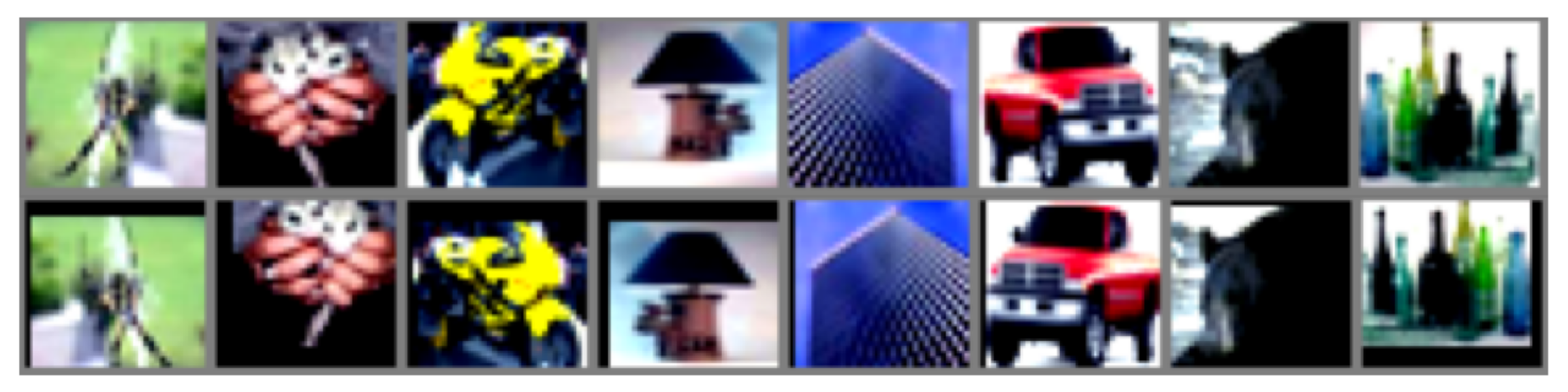
The CIFAR-100 [41] dataset consists of 50,000 training images and 10,000 test 32 × 32 color images in 100 classes, with 600 images per class in total. Some samples are shown in Figure 3. A random horizontal flip and crop with four-pixel zero-padding were carried out for data augmentation in the training procedure. Our experiments’ networks were all implemented strictly as their official papers without modification, including ResNet [1] (ResNet56, ResNet110, ResNet164), PreActResNet [32] (Pre110, Pre164), and WideResNet [33] (WRN-40-4, WRN-28-10).

For all runs, including the baselines, we trained a total epoch of 200, with a batch size of 128. The initial learning rate of 0.1 decreased to 0.0001 with cosine annealing. The SGD optimizer was used with a weight decay of 0.0005, and the momentum was set to 0.9. We adopted the last epoch model’s test set error rate as the reported results because choosing the best epoch results is prone to benefit unstable and oscillating configurations. To make the conclusion more concrete, each shown error rate in

Table 1. Test set error rate comparison on the CIFAR-100 dataset. The “BL” in the table’s column head is short for “baseline”. The results with no improvement compared to the baselines are underlined, and the bold results are the best ones for every network. The relative error rate drop of LSR-OS-TC compared to the baseline is shown in the brackets.

Model	Size	BL	LSR [19]	Tf-KD [27]	LSR-OS	LSR-OS-TC
ResNet56 [1]	0.9M	27.56	27.12	27.25	27.34	27.33 (0.23)
ResNet110	1.7M	25.79	25.48	25.45	25.60	25.43 (0.36)
Pre110 [32]	1.7M	25.63	25.49	25.46	25.42	25.52 (0.11)
ResNet164	1.7M	23.76	23.44	22.76	22.89	22.51 (1.25)
Pre164	1.7M	22.37	22.33	22.01	22.08	22.24 (0.13)
WRN-40-4 [33]	9.0M	20.73	20.96	20.56	20.71	20.52 (0.21)
WRN-28-10	36.5M	19.25	20.08	19.23	19.32	18.96 (0.29)

is the mean of four runs’ results with the identical setting.

5.1.1. Results Comparison

Table 1 shows that LSR works well on shallow networks while struggling to improve deeper networks where the knowledge distillation methods perform much better. For both LSR-OS-TC and Tf-KD, the manually designed teacher is a regularizing term that does not cost extra computational resources. However, Tf-KD needs several runs to confirm the best hyperparameters for every specific model, whereas our method LSR-KD-TC can work consistently on different models with the same parameters. The comparison of Tf-KD and LSR-OS reveals that a softer temperature $\tau$ in the LSR-OS is critical for teacher-free knowledge distillation. The further improvement obtained by LSR-OS-TC indicates the effectiveness of our two-component decomposition.

5.1.2. Training Detail

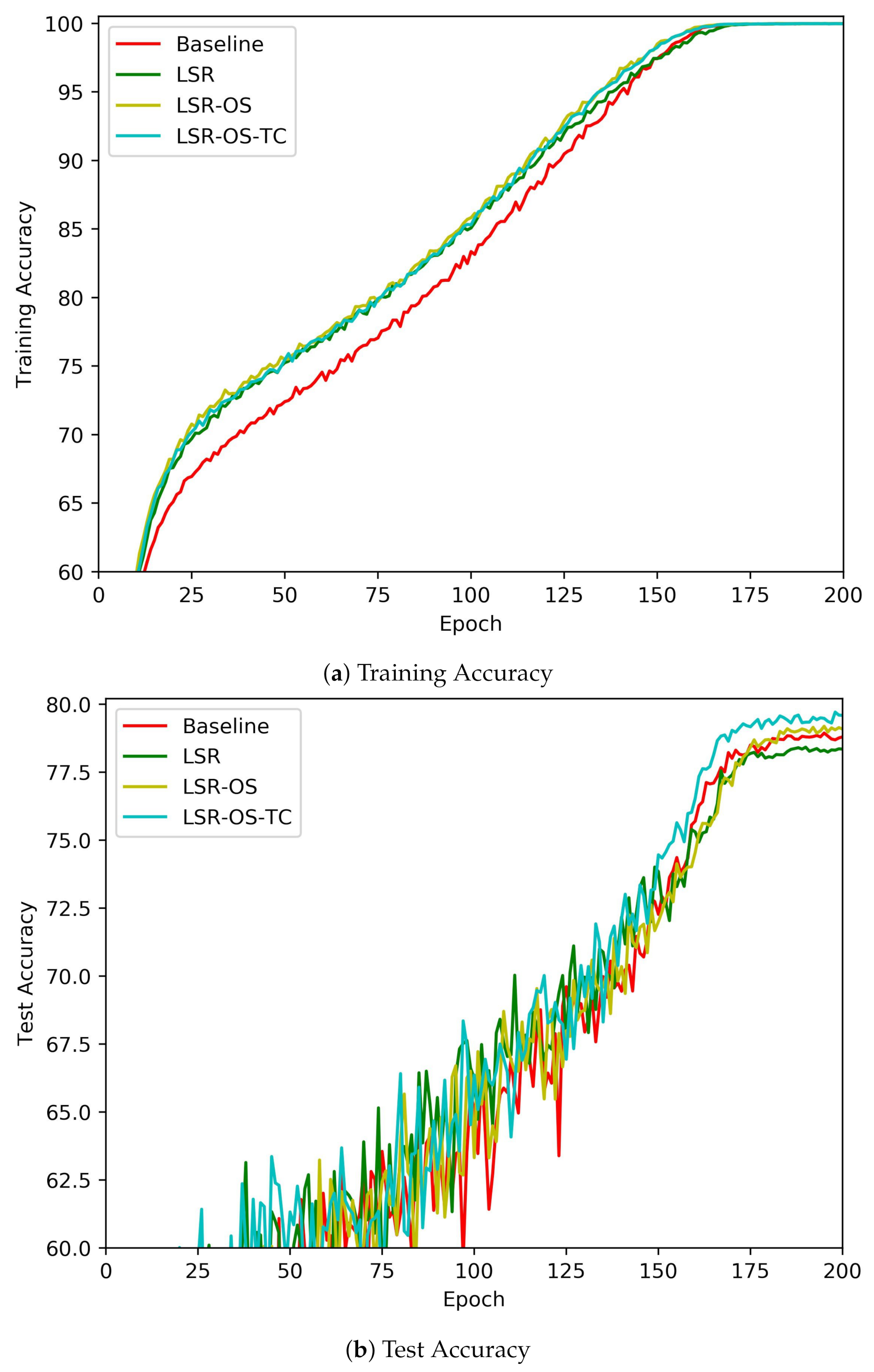
This subsection demonstrates the training curves of the proposed methods on the CIFAR-100 dataset with the WRN-40-4 network [33]. The implementation details are introduced at the beginning of Section 4.1. The accuracy curves on the training and test dataset are visualized in Figure 4. As Figure 4b shows, the LSR failed to improve the baseline test set accuracy on the WRN-40-4 network, whereas LSR-OS succeeded. With the modified teacher, LSR-OS-TC can improve the performance further.

Figure 5a,b illustrates the cross-entropy and KL-divergence loss of the training set, and Figure 5c shows the cross-entropy loss on the test set. Note that for LSR, we utilized the reformulated LSR-OS version with $\tau$ equal to one. The curves in Figure 4 and Figure 5 reveal a wealth of information.

With a stronger regularization effect, KD methods have a higher cross-entropy loss on both the training and test datasets. Figure 4a and Figure 5a show that, although all the regularization methods make the classification cross-entropy loss higher, their training accuracy is increased. This observation demonstrates that the regularization methods even generalize better on the training dataset.

Figure 5a shows the cross-entropy loss of multiple methods. The teacher correction method can effectively reduce the corresponding cross-entropy loss. Figure 5b gives the KL-divergence loss. We computed the KL-divergence between the output and a uniform distribution as LSR without using it in backpropagation for the baseline. Comparing to the baseline, the lower KL-divergence loss of LSR presents the regularization effect. The loss is further reduced on LSR-OS by choosing a softmax temperature larger than one (Figure 1f). LSR-OS-TC further reduces the loss by learning from a clearer teacher than the uniform distribution (Figure 1g).

5.2. CIFAR-10 and CINIC-10

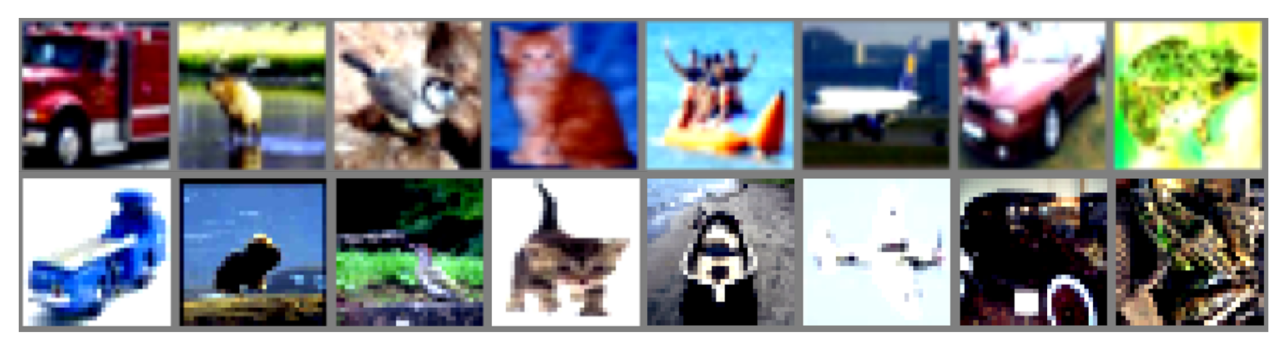
In the CIFAR-10 dataset experiments, the official division of the training data and test data was used, consisting of 50,000 images and 10,000 images, respectively, with a resolution of 32 × 32. As Figure 6 shows, the CINIC-10 dataset is an extended version of CIFAR-10. It contains all images from the CIFAR-10 dataset and derives 210,000 images downsampled to 32 × 32 from the ImageNet dataset. Similar to the CIFAR-100 implementation, a random horizontal flip and crop with four-pixel zero-padding were applied for the training set.

For CIFAR-10 and CINIC-10, we used the same hyperparameters as CIFAR-100 to maintain universality. We believe that there would be better results on both datasets through a more thorough search than we report in this paper.

Table 2. Test set error rate comparison on the CIFAR-10 dataset.

Model	Size	BL	LSR [19]	Tf-KD [27]	LSR-OS	LSR-OS-TC
ResNet20 [1]	0.3M	7.50	7.32	7.46	7.21	7.33 (0.17)
ResNet56	0.9M	5.83	5.98	5.57	5.77	5.41 (0.42)
ResNet164	1.7M	5.16	5.22	5.01	5.21	5.06 (0.10)
WRN-16-8 [33]	11.0M	4.17	3.96	3.85	3.88	3.73 (0.44)

and

Table 3. Test set error rate comparison on the CINIC10 dataset.

Model	Size	BL	LSR [19]	Tf-KD [27]	LSR-OS	LSR-OS-TC
ResNet20 [1]	0.3M	17.26	17.16	16.91	16.94	16.78 (0.48)
ResNet56	0.9M	15.27	15.39	15.12	15.17	15.04 (0.23)
ResNet164	1.7M	13.41	13.61	13.38	13.42	13.31 (0.10)
WRN-16-8 [33]	11.0M	11.52	11.22	11.15	11.13	11.01 (0.51)

show similar improvements to Table 1. The LSR method only helps half of the networks with tiny improvements, whereas our methods perform better. Most networks benefit from our methods. Note that the improvements of ResNet164 on both datasets are marginal. Similarly, on CIFAR-100, no significant improvement was observed on networks Pre110 and Pre164. We argue that the original LSR method on those networks is non-effective, and the tuned Tf-KD does not obtain better performance. Teacher-free knowledge distillation methods based on LSR have their intrinsic limitations, and they do not work universally on arbitrary networks. On those networks that LSR-OS-TC does no show obvious effect, one may try other types of KD methods with external knowledge [14,15,16,38,39]; yet, those methods may consume much more computational resource.

Compared to Table 1, the more underlines in Table 2 and Table 3 indicate a worse performance on CIFAR-10 and CINIC-10. We supposed two reasons: (1) the networks distill less information on 10-class datasets problems; (2) the gap between the test and training error rate on CIFAR-10 and CINIC-10 is lower than on CIFAR-100; then, the KD methods’ generalization effect is not significant.

5.3. GTZAN

GTZAN is a benchmark dataset for music genre classification collected by Tzanetakis and Cook [34]. Ten thousand song excerpts are included in ten genres: blues, jazz, classical, reggae, disco, country, hip hop, metal, pop, and rock. Each song is around 30 s and sampled at 22,050 Hz, 16 bits.

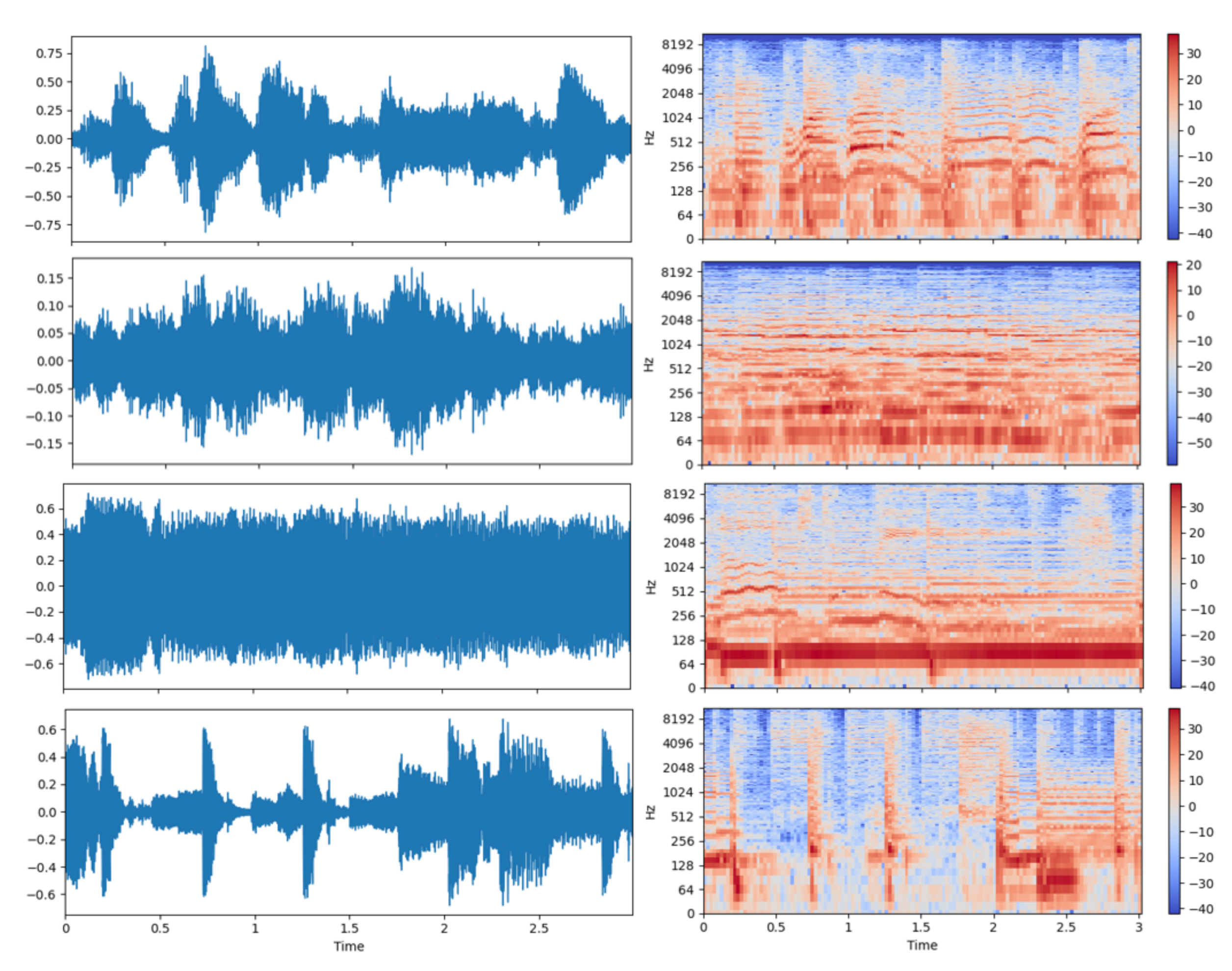
The dataset is split into 8/1/1 training, validation, and test. The number of songs for different genres in the training, validation, and test set is balanced. A 30 s song is cut into three-seconds clips with 50% overlap. Then, the STFT spectrogram on frames of length 1024 with an overlap of 50% is calculated. The final dimension of the three-seconds clip feature is 513 × 129. Some raw audio waves and their extracted STFT features are shown in Figure 7.

The networks nnet1 and nnet2 from Zhang et al. [42] were used as the baseline to evaluate the methods proposed in this paper. We ran a total epoch of 100, with a batch size of 128. The learning rate was set to 0.005. The SGD optimizer was used with a weight decay of 0.0005 and momentum of 0.9. The classification error was used as the measure of the performance, and all the results reported below were averaged over ten runs.

5.3.1. Result Comparison

In

Table 4. Test set error rate comparison on the GTZAN dataset. The column head “Clip” indicates the 3-second fragment results and under “Song” is the averaged total excerpt results.

Model	Size	Baseline		LSR [19]		Tf-KD [27]		LSR-OS		LSR-OS-TC
		Clip	Song	Clip	Song	Clip	Song	Clip	Song	Clip	Song
nnet1 [42]	0.46M	23.58	15.97	22.76	14.82	22.13	14.16	22.21	14.21	21.41 (2.17)	13.45 (2.52)
nnet2 [42]	1.25M	21.53	13.42	21.59	13.56	21.14	13.16	21.25	13.34	21.09 (0.44)	12.93 (0.49)

, we compare our work with other methods on the GTZAN dataset. We report both the single clip and the voted whole excerpt results. The LSR method reduces the nnet1 error rate by 1.15% and fail to improve nnet2. Tf-KD and our method LSR-OS achieve comparable improvement, while LSR-OS is easier to tune. LSR-OS with teacher correction improves both networks further.

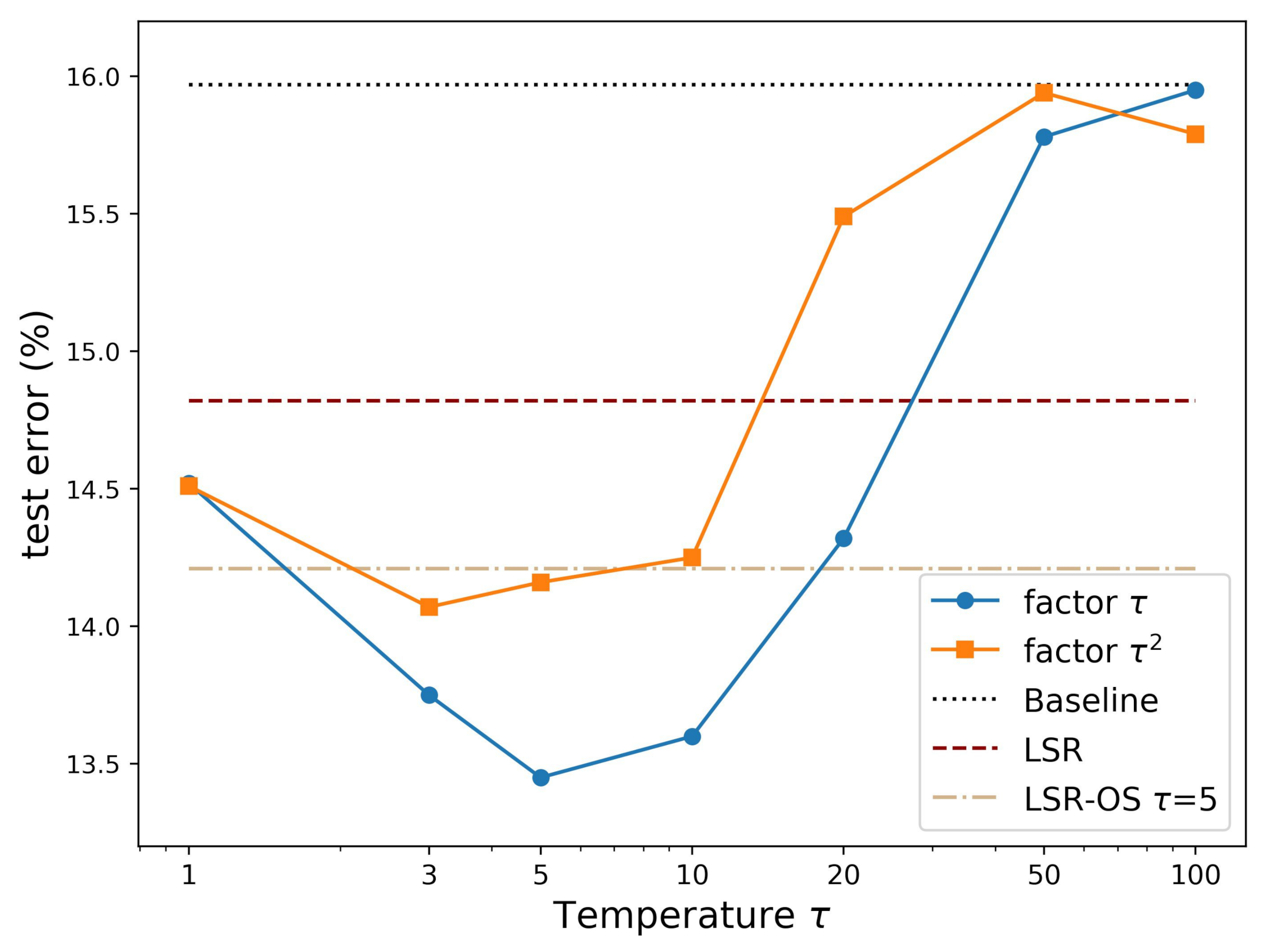
5.3.2. The Influence of Temperature on Teacher Correction

At the end of Section 3.3, we provide two inferences from the gradient conduction of teacher correction KL-loss. The gradient with the change of $\tau$ is stabilized by multiplying a factor $\tau$ with the KL-loss instead of ${\tau }^2$ in the traditional KD methods. On the other hand, the temperature $\tau$ needs to be low because a high temperature will make the gradient a constant related to the teacher distribution p${}^{\prime }$ and independent of the model output (Equation (14)).

Figure 8 confirms our inferences. In the experiments of Figure 8, the teacher correction $\gamma$ is set to 0.25. LSR-OS-TC with factor $\tau$ (blue line) performs significantly better than ${\tau }^2$ (orange line). Meanwhile, if the temperature is too high, the KL-loss would be noneffective, and the error rate is reduced to a similar value as the baseline, which is much worse than the LSR method.

6. Conclusions

Label smoothing is a critical regularization method for classification problems. The equivalence of LSR and knowledge distillation has caught the attention of researchers recently. In this paper, we proposed a simple, but effective teacher-free knowledge distillation method, LSR-OS-TC, without external knowledge or data, specifically LSR-OS-TC with a softer temperature model output and a manually designed teacher. We also analyzed the gradient of KL-loss in the LSR-OS-TC method and stated two matters that need attention for KD methods with manually designed teachers: multiplying $\tau$ instead of ${\tau }^2$ with the KL-loss and using a lower temperature. Experiments showed that LSR-OS-TC can perform consistently among models and datasets with the same hyperparameters. This consistency indicates that LSR-OS-TC can be a reliable substitution of label smoothing regularization. We believe that LSR-OS-TC is applicable to existing classification problems like speech recognition [23] and machine translation [24] directly and improves the performance more than LSR.

References

- He, K.; Zhang, X.; Ren, S.; Sun, J. Deep residual learning for image recognition. In Proceedings of the IEEE Conference on Computer Vision and Pattern Recognition, Las Vegas, NV, USA, 27–30 June 2016; pp. 770–778. [Google Scholar]
- Huang, G.; Liu, Z.; Pleiss, G.; Van Der Maaten, L.; Weinberger, K. Convolutional Networks with Dense Connectivity. IEEE Trans. Pattern Anal. Mach. Intell. 2019. [Google Scholar] [CrossRef] [PubMed] [Green Version]
- Chen, Y.; Li, J.; Xiao, H.; Jin, X.; Yan, S.; Feng, J. Dual path networks. In Proceedings of the Advances in Neural Information Processing Systems, Long Beach, CA, USA, 4–9 December 2017; pp. 4467–4475. [Google Scholar]
- Howard, A.G.; Zhu, M.; Chen, B.; Kalenichenko, D.; Wang, W.; Weyand, T.; Andreetto, M.; Adam, H. MobileNets: Efficient Convolutional Neural Networks for Mobile Vision Applications. arXiv 2017, arXiv:1704.04861. [Google Scholar]
- Sandler, M.; Howard, A.; Zhu, M.; Zhmoginov, A.; Chen, L.C. Mobilenetv2: Inverted residuals and linear bottlenecks. In Proceedings of the IEEE Conference on Computer Vision and Pattern Recognition, Salt Lake City, UT, USA, 18–23 June 2018; pp. 4510–4520. [Google Scholar]
- Howard, A.; Sandler, M.; Chu, G.; Chen, L.C.; Chen, B.; Tan, M.; Wang, W.; Zhu, Y.; Pang, R.; Vasudevan, V.; et al. Searching for MobileNetV3. In Proceedings of the 2019 IEEE/CVF International Conference on Computer Vision (ICCV), Seoul, Korea, 27 October–2 November 2019; pp. 1314–1324. [Google Scholar]
- Ma, N.; Zhang, X.; Zheng, H.T.; Sun, J. Shufflenet v2: Practical guidelines for efficient cnn architecture design. In Proceedings of the European Conference on Computer Vision (ECCV), Munich, Germany, 8–14 September 2018; pp. 116–131. [Google Scholar]
- Liu, H.; Simonyan, K.; Yang, Y. DARTS: Differentiable Architecture Search. arXiv 2019, arXiv:1806.09055. [Google Scholar]
- Tan, M.; Le, Q. EfficientNet: Rethinking Model Scaling for Convolutional Neural Networks. In Proceedings of the 36th International Conference on Machine Learning, Long Beach, CA, USA, 9–15 June 2019; Volume 97, pp. 6105–6114. [Google Scholar]
- Li, H.; Kadav, A.; Durdanovic, I.; Samet, H.; Graf, H.P. Pruning Filters for Efficient ConvNets. arXiv 2016, arXiv:1608.08710. [Google Scholar]
- Rastegari, M.; Ordonez, V.; Redmon, J.; Farhadi, A. Xnor-net: Imagenet classification using binary convolutional neural networks. In Proceedings of the European conference on computer vision, Amsterdam, The Netherlands, 11–14 October 2016; pp. 525–542. [Google Scholar]
- Han, S.; Mao, H.; Dally, W.J. Deep Compression: Compressing Deep Neural Networks with Pruning, Trained Quantization and Huffman Coding. arXiv 2015, arXiv:1510.00149. [Google Scholar]
- Hinton, G.; Vinyals, O.; Dean, J. Distilling the Knowledge in a Neural Network. arXiv 2015, arXiv:1503.02531. [Google Scholar]
- Furlanello, T.; Lipton, Z.C.; Tschannen, M.; Itti, L.; Anandkumar, A. Born Again Neural Networks. arXiv 2018, arXiv:1805.04770. [Google Scholar]
- Zhang, Y.; Xiang, T.; Hospedales, T.M.; Lu, H. Deep Mutual Learning. In Proceedings of the IEEE Conference on Computer Vision and Pattern Recognition (CVPR), Salt Lake City, UT, USA, 18–23 June 2018. [Google Scholar]
- Zhang, L.; Song, J.; Gao, A.; Chen, J.; Bao, C.; Ma, K. Be Your Own Teacher: Improve the Performance of Convolutional Neural Networks via Self Distillation. In Proceedings of the IEEE/CVF International Conference on Computer Vision (ICCV), Seoul, Korea, 27 October–2 November 2019. [Google Scholar]
- Yun, S.; Park, J.; Lee, K.; Shin, J. Regularizing Class-Wise Predictions via Self-Knowledge Distillation. In Proceedings of the IEEE/CVF Conference on Computer Vision and Pattern Recognition (CVPR), Seattle, WA, USA, 14–19 June 2020. [Google Scholar]
- Hendrycks, D.; Mu, N.; Cubuk, E.D.; Zoph, B.; Gilmer, J.; Lakshminarayanan, B. AugMix: A Simple Method to Improve Robustness and Uncertainty under Data Shift. In Proceedings of the International Conference on Learning Representations, Virtual Conference, 26–30 April 2020. [Google Scholar]
- Szegedy, C.; Vanhoucke, V.; Ioffe, S.; Shlens, J.; Wojna, Z. Rethinking the Inception Architecture for Computer Vision. In Proceedings of the IEEE Conference on Computer Vision and Pattern Recognition (CVPR), Las Vegas, NV, USA, 26 June 2016. [Google Scholar]
- Zoph, B.; Vasudevan, V.; Shlens, J.; Le, Q.V. Learning transferable architectures for scalable image recognition. In Proceedings of the IEEE Conference on Computer Vision and Pattern Recognition, Salt Lake City, UT, USA, 18–23 June 2018; pp. 8697–8710. [Google Scholar]
- Real, E.; Aggarwal, A.; Huang, Y.; Le, Q.V. Regularized evolution for image classifier architecture search. In Proceedings of the AAAI Conference on Artificial Intelligence, Honolulu, HI, USA, 27 January 2019; Volume 33, pp. 4780–4789. [Google Scholar]
- Huang, Y.; Cheng, Y.; Bapna, A.; Firat, O.; Chen, D.; Chen, M.; Lee, H.; Ngiam, J.; Le, Q.V.; Wu, Y.; et al. Gpipe: Efficient training of giant neural networks using pipeline parallelism. In Proceedings of the Advances in Neural Information Processing Systems, Vancouver, BC, Canada, 8–14 December 2019; pp. 103–112. [Google Scholar]
- Chorowski, J.; Jaitly, N. Towards Better Decoding and Language Model Integration in Sequence to Sequence Models. In Proceedings of the Interspeech, Stockholm, Sweden, 20 August 2017. [Google Scholar]
- Vaswani, A.; Shazeer, N.; Parmar, N.; Uszkoreit, J.; Jones, L.; Gomez, A.N.; Kaiser, L.; Polosukhin, I. Attention is All you Need. arXiv 2017, arXiv:1706.03762. [Google Scholar]
- Xu, Y.; Xu, Y.; Qian, Q.; Li, H.; Jin, R. Towards Understanding Label Smoothing. arXiv 2020, arXiv:2006.11653. [Google Scholar]
- Pereyra, G.; Tucker, G.; Chorowski, J.; Kaiser, Ł.; Hinton, G. Regularizing Neural Networks by Penalizing Confident Output Distributions. arXiv 2017, arXiv:1701.06548. [Google Scholar]
- Yuan, L.; Tay, F.E.H.; Li, G.; Wang, T.; Feng, J. Revisit Knowledge Distillation: A Teacher-free Framework. arXiv 2019, arXiv:1909.11723. [Google Scholar]
- Zhang, Z.; Sabuncu, M. Self-Distillation as Instance-Specific Label Smoothing. In Advances in Neural Information Processing Systems; Larochelle, H., Ranzato, M., Hadsell, R., Balcan, M.F., Lin, H., Eds.; Curran Associates, Inc.: Red Hook, NY, USA, 2020; Volume 33, pp. 2184–2195. [Google Scholar]
- Tang, J.; Shivanna, R.; Zhao, Z.; Lin, D.; Singh, A.; Chi, E.H.; Jain, S. Understanding and Improving Knowledge Distillation. arxiv 2020, arXiv:2002.03532. [Google Scholar]
- Krizhevsky, A.; Nair, V.; Hinton, G. CIFAR-10 (Canadian Institute for Advanced Research). Available online: http://www.cs.toronto.edu/~kriz/cifar.html (accessed on 18 January 2021).
- Darlow, L.N.; Crowley, E.J.; Antoniou, A.; Storkey, A.J. CINIC-10 is not ImageNet or CIFAR-10. arXiv 2018, arXiv:1810.03505. [Google Scholar]
- He, K.; Zhang, X.; Ren, S.; Sun, J. Identity mappings in deep residual networks. In Proceedings of the European Conference on Computer Vision, Amsterdam, The Netherlands, 11–14 October 2016; pp. 630–645. [Google Scholar]
- Zagoruyko, S.; Komodakis, N. Wide Residual Networks; BMVC: York, UK, 2016. [Google Scholar]
- Tzanetakis, G.; Cook, P. Musical genre classification of audio signals. IEEE Trans. Speech Audio Process. 2002, 10, 293–302. [Google Scholar] [CrossRef]
- Wang, L.; Yoon, K.J. Knowledge Distillation and Student-Teacher Learning for Visual Intelligence: A Review and New Outlooks. IEEE Trans. Pattern Anal. Mach. Intell. 2021, 1. [Google Scholar] [CrossRef]
- Jin, X.; Peng, B.; Wu, Y.; Liu, Y.; Liu, J.; Liang, D.; Yan, J.; Hu, X. Knowledge Distillation via Route Constrained Optimization. In Proceedings of the IEEE/CVF International Conference on Computer Vision (ICCV), Seoul, Korea, 27 October–2 November 2019. [Google Scholar]
- Luan, Y.; Zhao, H.; Yang, Z.; Dai, Y. MSD: Multi-Self-Distillation Learning via Multi-classifiers within Deep Neural Networks. arXiv 2019, arXiv:1911.09418. [Google Scholar]
- Song, G.; Chai, W. Collaborative learning for deep neural networks. In Proceedings of the Advances in Neural Information Processing Systems, Montréal, QC, Canada, 2–8 December 2018; pp. 1832–1841. [Google Scholar]
- Xu, L.; Zhu, X.; Gong, S. Knowledge distillation by on-the-fly native ensemble. In Proceedings of the Advances in Neural Information Processing Systems, Montréal, QC, Canada, 2–8 December 2018; pp. 7517–7527. [Google Scholar]
- Müller, R.; Kornblith, S.; Hinton, G.E. When Does Label Smoothing Help? NeurIPS: Vancouver, BC, Canada, 2019. [Google Scholar]
- Krizhevsky, A. Learning Multiple Layers of Features from Tiny Images; Technical Report; University of Toronto: Toronto, ON, Canada, 2009. [Google Scholar]
- Zhang, W.; Lei, W.; Xu, X.; Xing, X. Improved music genre classification with convolutional neural networks. Proc. Interspeech 2016, 2016, 3304–3308. [Google Scholar]
Figure 1.
Graphical illustration of different methods. (a) Knowledge distillation for model compression; (b) traditional classification framework with cross-entropy loss; (c) label smoothing regularization; (d) label smoothing regularization in the KD form; (e) teacher-free knowledge distillation; (f) our proposed LSR-OS; (g) LSR-OS with teacher correction.
Figure 2.
Comparison of the soft model output of LSR-OS at different temperatures . C8 is the predicted class. (a) Soft model distribution comparison; (b) corresponding KL-loss between different temperature outputs and the uniform distribution; (c) KL-loss multiplied by a factor .
Figure 3.
The typical images from the CIRFAR-100 dataset. (Top): original image. (Bottom): augmented image. The labels from left to right: spider, possum, motorcycle, lamp, skyscraper, pickup truck, bear, and bottle.
Figure 4.
The accuracy curves for training on the CIRFAR100 dataset with the WRN-40-4 network.
Figure 5.
The loss curves for training on the CIRFAR100 dataset with the WRN-40-4 network.
Figure 6.
The typical images from the CINIC-10 dataset. Top: inherited from the CIFAR-10 dataset. Top: extended from the ImageNet dataset. The labels from left to right: truck, deer, bird, cat, ship, plane, car, and frog.
Figure 7.
The three-seconds music clips from the GTZAN dataset. Left: the raw waveform data. Right: the corresponding STFT spectrogram in the log scale y-axis. The music genre from top to bottom: blues, classical, country, and disco.
Figure 8.
Graph of test error vs. temperature of nnet1 on the GTZAN dataset. Blue: LSR-OS-TC with factor ; orange: LSR-OS-TC with factor .