Fragility Curves and Probabilistic Seismic Demand Models on the Seismic Assessment of RC Frames Subjected to Structural Pounding

Abstract

This study aims to evaluate five different methodologies reported in the literature for developing fragility curves to assess the seismic performance of RC structures subjected to structural pounding. In this context, displacement-based and curvature-based fragility curves are developed. The use of probabilistic seismic demand models (PSDMs) on the fragility assessment of the pounding risk is further estimated. Linear and bilinear PSDMs are developed, while the validity of the assumptions commonly used to produce a PSDM is examined. Finally, the influence of the PSDMs’ assumptions on the derivation of fragilities for the structural pounding effect is identified. The examined pounding cases involve the interaction between adjacent RC structures that have equal story heights (floor-to-floor interaction). Results indicate that the fragility assessment of the RC structure that suffers the pounding effect is not affected by the examined methodologies when the performance level that controls the seismic behavior is exceeded at low levels of IM. Thus, the more vulnerable the structure is due to the pounding effect, the more likely that disparities among the fragility curves of the examined methods are eliminated. The use of a linear PSDM fails to properly describe the local inelastic demands of the structural RC member that suffers the impact effect. The PSDM’s assumptions are not always satisfied for the examined engineering demand parameters of this study, and thus may induce errors when fragility curves are developed. Nevertheless, errors induced due to the power law model and the homoscedasticity assumptions of the PSDM can be reduced by using the bilinear regression model.

1. Introduction

In the last three decades, several researches have been undertaken to address the seismic performance of structures through probabilistic procedures. A key issue in these methods is the definition of accurate fragility curves that identifies the vulnerability of structures to seismic damage. Withman et al. [1] introduced the concept of damage probability matrices (DPM) to provide the probability that a particular level of damage will occur to a structural system, while the ground motion has been described by the modified Mercalli intensity (MMI) scale. Thereafter, in 1991, the Applied Technology Council (ATC) and the Federal Emergency Management Agency (FEMA) introduced the use of vulnerability functions for lifelines in the ATC-25 report [2]. For this purpose, the concept of a continuous relation between the seismic damage and ground motion intensity is established and a regression analysis of different damage probability matrices is performed. In 1997, the risk assessment software package Hazard United States (HAZUS) was first introduced by the Federal Emergency Management Agency (FEMA). The HAZUS earthquake model consisted of an inventory data base, a ground motion model, an earthquake model of buildings, and lifelines damage models in order to evaluate the probability of damage to buildings and infrastructures according to ground shaking data from the U.S. Geological Survey (USGS) shake map [3]. Nowadays, fragility curves have been evolved as an efficient tool for retrofit and design of infrastructures [4].

Different types of fragility curves have been reported in the literature, namely expert-based opinion, experimental, analytical, hybrid, and empirical curves. Expert opinion fragility curves are developed based on statistics estimations of the probable damage when different earthquake intensities occur. ATC-13 [5] developed DPMs for typical California infrastructures using MMIs based on opinion of 42 experts. In 2007, Kostov et al. [6] developed vulnerability curves for Sofia’s buildings stock and lifelines according to European Macro Seismic Scale (EMS98). Nevertheless, the reliability of this type of fragility curves is questionable due to uncertainties contain the experts’ judgements [7]. Empirical fragility curves are developed based on damage observations from past earthquakes. Basöz et al. [8] assessed the vulnerability of bridges based on the observed data of Loma Prietta 1989, and Northridge 1994 developed empirical fragility curves through logistic regression. In 2003, Rosseto and Elanshai [7] developed empirical fragility curves based on a database of 99 post-earthquake damage distributions observed in 19 earthquakes of 340,000 RC buildings. Other researchers [9,10,11] have also used post-earthquake damage data to develop empirical curves. On the other hand, the experimental fragilities are based on experimental results. Vosooghi and Saidi [12] developed experimental fragility curves for bridge piers based on shake table and cyclic load tests. They correlate the damage state and the damage index to develop fragility functions. In the case of absence of damage data from real earthquakes, analytical fragility curves can be developed using results of structural demands from analytical simulations of non-linear static analysis [13,14,15], non-linear dynamic analysis [16,17,18,19,20,21,22,23,24,25], and elastic spectral analysis [26,27]. Finally, the hybrid method uses a combination of different procedures (available damage statistics and nonlinear analysis) for the prediction of the damage levels. Kappos et al. [28,29] developed DPMs where part of intensity levels was constructed using available data from past earthquakes and results based on nonlinear dynamic analyses. In 2006, Kappos et al. [30] presented fragility curves for masonry and RC buildings combining statistical data derived from earthquake-damage Greek buildings and results of nonlinear static or dynamic analyses.

In order to develop fragility curves, the structural demands, the earthquake intensity measures, and uncertainties regarding demand and capacity have to be defined. Focused on the development of analytical fragility curves non-linear dynamic analysis procedures have to be performed. Thus, the influence of the record-to-record variability on structural seismic response is taken into account, as the structural model is subjected to a wide range of ground motions. The characteristics of ground motions are described through intensity measures (IMs) while the structural behavior through engineering demand parameters (EDPs). Nonlinear dynamic analysis procedures, such as cloud analysis (CA) [31,32,33], incremental dynamic analysis (IDA) [34], and multi-stripe analysis (MSA) [35,36], can be performed to generate samples of EDPs-IMs pairs.

Thereafter, the discrete probability data points for each level of earthquake intensity can be defined incorporating directly the results of the nonlinear analyses (e.g., IDA) in order to provide a form of empirical cumulative distribution function (CDF) of fragility curve. A key parameter for the development of a fragility curve is the definition of the median (μ) and the dispersion (β) of the EDP-IM values, and thus different approaches have been reported in the literature. Among them, the moment method, the method of maximum likelihood estimation, the IM percentiles method, and the concept of the probabilistic seismic demand model (PSDM) are widely used [37,38,39,40]. For the moment method (also known as Method A by Porter) [37], parameters of the fragility curves occur based on the earthquake intensities of the observed data. Baker [38] introduced the method of maximum likelihood estimation where the parameters of the fragility curves are deduced through maximizing the likelihood of producing the observed data. The IM percentiles [39] incorporate results of the IDA and are based on the summarized 16%, 50%, and 84% IDA curves, respectively. Cornel et al. [31] introduced the relationship between the IM and EDP that provides a closed form solution of fragility curves. In this method, the variation of the structural demand for a wide range of earthquake intensities can be described through regression models known as the probabilistic seismic demand model (PSDM). In this context, the linear regression model is commonly used. Nevertheless, when nonlinear seismic demands have to be described, the use of bilinear PSDM is suggested [40]. Ramammothy et al. [41] developed fragility curves based on linear and bilinear PSDMs for the vulnerability assessment of RC buildings and the evaluation of retrofitted strategy. Bai et al. [42] developed linear and bilinear PSDMs in order to achieve a better representation of the demand for the examined range of the IM. Freddi et al. [43] used bilinear PSDM to describe the local EDPs of low-ductility RC frames. Aljawhari et al. [44] used bilinear PSDM to study the influence of ground motion sequences on the fragility of RC moment-resisting frames. Other researchers developed fragility curves based on a Bayessian approach for the formulation of PSDMs [41,42,45,46]. Furthermore, Jalayer et al. [47] introduced a robust fragility assessment approach for the RC moment-resisting frame using Markov Chain Monte Carlo (MCMC) simulation.

Recently, fragility curves have also been used for the probabilistic evaluation of the pounding effect between adjacent buildings. Tubaldi et al. [40] developed fragility curves for the assessment of the seismic pounding risk of singe-degree-of-freedom (SDOF) and multi-degree-of-freedom (MDOF) systems, based on linear and bilinear PSDMs. Nazri et al. [48] developed fragility curves in terms of maximum interstory drift vs. PGA to study the structural pounding effect between the adjacent RC frames, taking into account the available separation distance and the structural irregularities. The results of the assessment were based on the IDA method. Ιn 2020, Flegga and Favvata [49] investigated the floor-to-floor structural pounding effect between RC structures at different global and local performance levels as a function of PGA and the spectral acceleration, Sa. Kazemi et al. [50] studied the effect of the floor-to-floor structural pounding between RC and steel moment resisting frames (MRFs) at different global performance levels. Fragility curves based on IDA have been developed in terms of maximum interstory drift as a function of Sa. Finally, Flenga and Favvata [51] incorporated the local inelastic demands of a RC frame in the probabilistic assessment of the pounding risk. The floor-to-floor and the floor-to-column types of structural pounding were evaluated based on fragilities that have been developed through linear and bilinear PSDMs.

Based on this review, it can be stated that, although many different probabilistic methods have been proposed for the derivation of accurate fragility curves, a limited number of methodologies in the research area of the pounding risk between adjacent structures has been evaluated.

So, this study aims to evaluate five different methodologies reported in the literature for developing fragility curves to assess the seismic performance of real RC structures subjected to structural pounding. In this context, displacement-based and curvature-based fragility curves are developed. The validity of the assumptions commonly used to produce a PSDM is examined, and the influence of these assumptions on the derivation of the fragilities for the structural pounding effect is identified. EDPs of the RC structure that suffers the pounding effect have been estimated based on the results of IDAs [34].

2. Methodologies of Developing Fragility Curves

In modern seismic engineering, fragility curves are employed to assess the vulnerability of a structure due to seismic events. Fragility curves describe the probability an engineering demand parameter (EDP) to exceed the capacity level of $\hat{\mathrm{C}}$ for a given IM, and can be calculated as:

$$\mathrm{P}\left[\mathrm{EDP}|\mathrm{IM}\ge \mathrm{C}|\mathrm{IM}\right]=\mathsf{\Phi }\left(\frac{\ln \mathsf{\mu }-\ln \hat{\mathrm{C}}}{\mathsf{\beta }}\right)$$

(1)

The fragility assessment of the pounding effect is examined considering the following five methods:

(a)

Empirical cumulative distribution function (CDF),

(b)

Moment method (MM),

(c)

Maximum likelihood estimation (MLE) method,

(d)

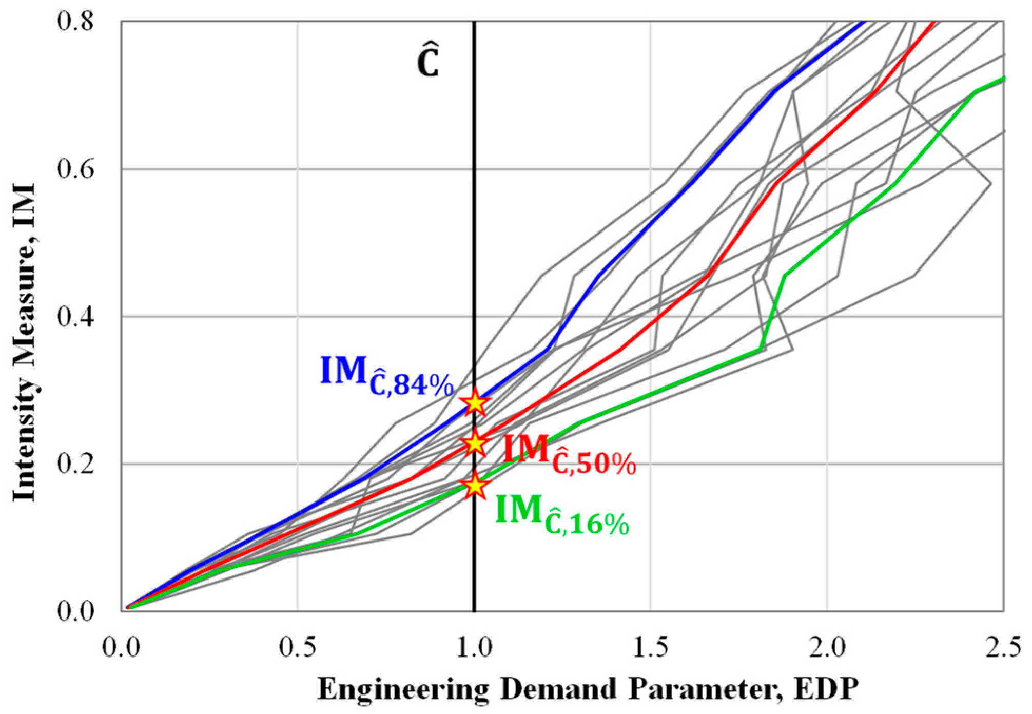
16%, 50%, 84% IM—percentiles, and

(e)

Probabilistic seismic demand model (PSDM).

The empirical CDF method provides discrete probability data points at a given value of IM. For a continuous representation of the fragility curve, the median (μ) and the dispersion (β) of the responses have to be defined utilizing one of the other four methodologies. All methods are presented and discussed below. Fragilities based on the empirical CDF method are considered as the reference probability data.

2.1. Empirical Cumulative Distribution Function (CDF)

The implementation of IDA method results to EDPs values that correspond to each seismic excitation for a given value of IM. Therefore, stripes of discrete EDPs values are generated at increasing levels of IM. The probability an EDP to exceed a particular performance level for a given value IM is estimated as the sum of those events which exceed the capacity $\hat{\mathrm{C}}$ over the total number of seismic excitations:

$$\mathrm{P}\left[\mathrm{EDP}\ge \widehat{\mathrm{C}}\right]=\frac{\mathrm{m}}{\mathrm{n}}$$

(2)

where m is the number of events which exceed a particular limit state (capacity level) $\hat{\mathrm{C}}$ at the level of IM, and n is the total number of seismic excitations.

In Figure 1, the IDA curves for n ground motions and the corresponding fragility curve based on the empirical CDF method are presented. In Figure 1a, dots represent the structural response at a particular value of IM, while the vertical solid line depicts the capacity $\hat{\mathrm{C}}$ at the performance level of the assessment. The red dots refer to the m events where the demand exceeds the capacity at the particular level of IM, while the blue dots refer to (n-m) events for which demand does not exceed capacity. The discrete probability data points (Figure 1b) at the performance level of $\hat{\mathrm{C}}$ can be evaluated based on Equation (2). Therefore, the fragility curve based on the empirical CDF can be developed by connecting the discrete points with linear segments. Tubaldi et al. [40] utilized the discrete probability data points to validate the fragility curves developed through PSDM for different values of separation gap distance.

2.2. Moment Method

The moment method is used to define the median (μ) and the dispersion (β) in the case of continuous representation of the fragility curve. This method is also known as “Method A” by Porter et al. [37] and is based on the results of the IDA method. For the calculation of median (μ) and dispersion (β) values of IM at the onset of exceedance, a particular limit state is used considering lognormal distribution. For each seismic motion, the value of IM at the capacity level $\hat{\mathrm{C}}$ is presented in Figure 2 with star point.

The μ and β can be estimated as:

$$\mathsf{\mu }=\frac{1}{\mathrm{n}}{\displaystyle \sum }_{\mathrm{i}=1}^{\mathrm{n}}{\mathrm{lnIM}}_{\mathrm{i}}$$

(3)

$$\mathsf{\beta }=\sqrt{\frac{1}{\mathrm{n}-1}{\displaystyle \sum }_{\mathrm{i}=1}^{\mathrm{n}}{\left(\ln \left({\mathrm{IM}}_{\mathrm{i}}\right)-\mathsf{\mu }\right)}^2}$$

(4)

where n is the number of seismic excitations and IM_i is the value of IM associated with the onset of exceedance a particular performance level. Aslani and Miranda [52] used this fitting approach to develop continuous fragility curves for different damage states in slab-column connections of non-ductile reinforced concrete buildings.

2.3. Maximum Likelihood Estimation (MLE) Method

The method of MLE [38] provides the median (μ) and dispersion (β) so that the fitted fragility function is more consistent with the probability data points obtained through Equation (2).

The likelihood function can be calculated as:

$$\mathrm{Likelihood}={\displaystyle \prod }_{\mathrm{j}=1}^{\mathrm{m}}\left(\begin{array}{c}{\mathrm{n}}_{\mathrm{j}}\\ {\mathrm{z}}_{\mathrm{j}}\end{array}\right)\mathsf{\Phi }{\left(\frac{\ln \left({\mathrm{IM}}_{\mathrm{j}}\right)-\mathsf{\mu }}{\mathsf{\beta }}\right)}^{{\mathrm{z}}_{\mathrm{j}}}{\left(1-\mathsf{\Phi }\left(\frac{\ln \left({\mathrm{IM}}_{\mathrm{j}}\right)-\mathsf{\mu }}{\mathsf{\beta }}\right)\right)}^{{\mathrm{n}}_{\mathrm{j}}{-\mathrm{z}}_{\mathrm{j}}}$$

(5)

where m is the number of IM levels, z_j is the number of ground motions that exceed a performance level out of n_j seismic excitations, and Π denotes a product over all the considered IM levels.

Through maximizing the likelihood function the median (μ) and dispersion (β), are defined as:

$${\{\mathsf{\mu },\mathsf{\beta }\}=\max }_{\mathsf{\mu },\mathsf{\sigma }}{\displaystyle \sum }_{\mathrm{j}=1}^{\mathrm{m}}\left\{\ln \left(\begin{array}{c}{\mathrm{n}}_{\mathrm{j}}\\ {\mathrm{z}}_{\mathrm{j}}\end{array}\right){+\mathrm{z}}_{\mathrm{j}}\ln \mathsf{\Phi }\left(\frac{\ln \left({\mathrm{IM}}_{\mathrm{j}}\right)-\mathsf{\mu }}{\mathsf{\beta }}\right){+(\mathrm{n}}_{\mathrm{j}}{-\mathrm{z}}_{\mathrm{j}})\ln \left(1-\mathsf{\Phi }\left(\frac{\ln \left({\mathrm{IM}}_{\mathrm{j}}\right)-\mathsf{\mu }}{\mathsf{\beta }}\right)\right)\right\}$$

(6)

Baker [38] introduced the method of maximum likelihood estimation to develop fragility curves when incremental analysis was performed up to some level of IM for some ground motions.

2.4. 16%, 50%, 84%. IM—Percentiles

IDAs curves define the seismic demands of the structural model for a suite of ground motions, so a deterministic evaluation of structural behavior is provided. The summarization of IDAs curves into a central value (mean or median) and a measure of dispersion quantifies the randomness introduced by records [34].

Each EDP|IM point at the summarized IDAs curves of 16%, 50%, and 84% represents an upper value of EDP where 16%, 50%, and 84% of the records produce demand lower of this value for a given level of IM. So, in the context of fragility curves, the 16%, 50%, and 84% percentiles curves are also defined in this study.

The median value μ is defined as the intersection of the 50% summarized IDA curve with the level of capacity $\hat{\mathrm{C}}$ (μ = ${\mathrm{IM}}_{\mathrm{c},50\%}$), while the dispersion β is calculated as [53]:

$$\mathsf{\beta }=\frac{1}{2}\ln \frac{{\mathrm{IM}}_{\mathrm{C},84\%}}{{\mathrm{IM}}_{\mathrm{C},16\%}}$$

(7)

where, ${\mathrm{IM}}_{\mathrm{C},84\%}$, ${\mathrm{IM}}_{\mathrm{C},16\%}$ are the intersections of the corresponding summarized IDAs curves with the capacity level of $\hat{\mathrm{C}}$ (see Figure 3). Freddi et al. [53] developed fragility curves for assessing the vulnerability of existing reinforced concrete buildings retrofitted by dissipated braces.

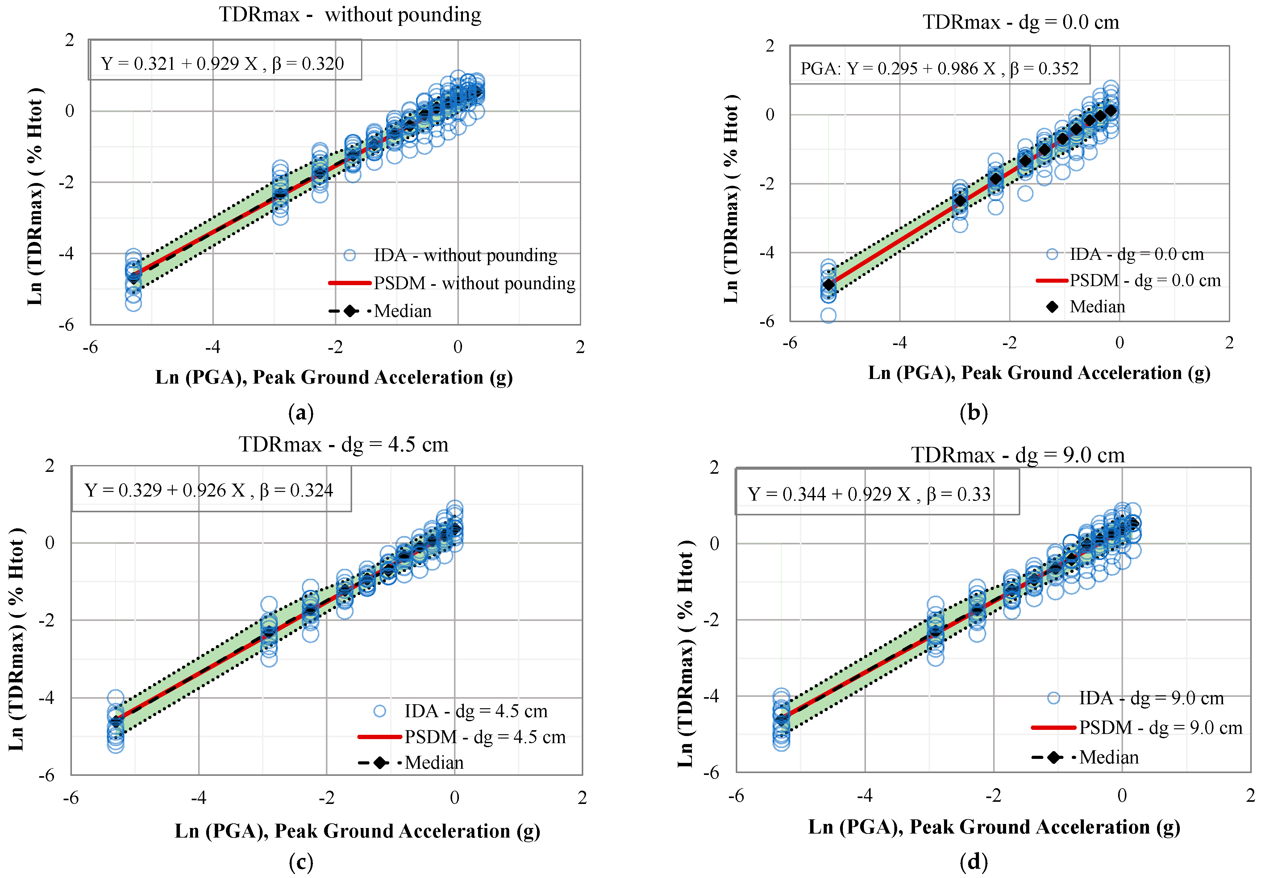
2.5. Probabilistic Seismic Demand Model (PSDM)

Another way of generating fragility curves is through the probabilistic seismic demand model [40,41,42,45,46,47,49,51]. A probabilistic seismic demand model is a mathematical relation between the structural response and the earthquake intensity measure (IM) [54]. The mathematical representation of the PSDM leads to a closed form solution that permits the definition of the fragility curves [31]. Therefore, Equation (1) is transformed to the following expression:

$${\mathrm{G}}_{\mathrm{EDP}|\mathrm{IM}}\left(\mathrm{C}\right|\mathrm{IM})=\mathrm{P}[\mathrm{EDP}|\mathrm{IM}\ge \mathrm{C}|\mathrm{IM}]=\mathsf{\Phi }\left(\frac{\ln \widehat{\mathrm{EDP}}|\mathrm{IM}-\ln \hat{\mathrm{C}}}{{\mathsf{\beta }}_{\mathrm{EDP}|\mathrm{IM}}}\right)$$

(8)

Φ(.) denotes the standard normal cumulative function, $\widehat{\mathrm{EDP}}|\mathrm{IM}$ the median structural demand, $\widehat{\mathrm{C}}$ the median value of the capacity, and β_EDP|IM the logarithm standard deviation.

The mathematical representation of median structural demand response $\widehat{\mathrm{EDP}}$ and the IM can be approximated by a two parameters power law model [31,55]:

$$\widehat{\mathrm{EDP}}{|\mathrm{IM}=\mathrm{a}\mathrm{IM}}^{\mathrm{b}}$$

(9)

The coefficients α and b are calculated through linear regression analysis of logarithm of IM and EDP, so the Equation (9) is transformed to the following expression:

$$\ln \widehat{\mathrm{EDP}}|\mathrm{IM}=\mathrm{blnIM}+\mathrm{lna}+\mathsf{\epsilon }|\mathrm{IM}$$

(10)

where, ε|IM is the random error with mean zero and variance σ².

The structural response demand is assumed to follow lognormal distribution [55] with logarithm standard deviation ${\mathsf{\beta }}_{\mathrm{EDP}|\mathrm{IM}}$ which is calculated by the following equation:

$${\mathsf{\beta }}_{\mathrm{EDP}|\mathrm{IM}}=\sqrt{\frac{{{\displaystyle \sum }}_{\mathrm{i}=1}^{\mathrm{n}}{\left({\mathrm{lnEDP}}_{\mathrm{i}}|\mathrm{IM}-\ln \widehat{\mathrm{EDP}}|\mathrm{IM}\right)}^2}{\mathrm{n}-2}}$$

(11)

Furthermore, a bilinear regression model is also considered to capture the nonlinear behavior of the structural members. The bilinear regression model can be described by the following expression:

$$\ln \widehat{\mathrm{EDP}}{|\mathrm{IM}=(\mathrm{a}}_1{+\mathrm{b}}_1{\mathrm{lnIM}\left)\right(1-\mathrm{H}}_1)+\left[{\mathrm{lnEDP}|\mathrm{IM}}^{*}{+\mathrm{b}}_2\left({\mathrm{lnIM}-\mathrm{lnIM}}^{*}\right)\right]{\mathrm{H}}_1+\mathsf{\epsilon }|\mathrm{IM}$$

(12)

The coefficients α₁, b₁, and b₂ are defined through linear regression analysis and determine the slope of the two linear branches. H₁ is a dummy variable which is equal to H₁ = 0 for IM ≤ IM* and H1 = 1 for IM > IM*. Finally, the parameter IM* is the intersection of two linear branches, while ${\mathrm{lnEDP}|\mathrm{IM}}^{*}$ is the value of the $\mathrm{EDP}$ at the intersection point.

3. Examined Case Study

3.1. Description

The probabilistic seismic assessment of an eight-story RC frame structure that suffers the impact effect from an adjacent three-story rigid structure (T_3-story = ∞) is evaluated. The story levels of the adjacent structures have the same height so that collisions may occur between the story diaphragms and consequently between the story masses (floor-to-floor interaction). The separation gap distance (d_g) between the adjacent structures is considered as: d_g = 0.0 cm (structures in contact from the beginning), d_g = 4.5 cm, and d_g = 9.0 cm (Eurocode’s requirement). The seismic performance of the eight-story structure without the pounding effect is also included for comparison reasons. The fundamental period of the eight-story RC frame is 1.132 s and the yield displacement at the top story level is equal to 5 cm. The two adjacent buildings are considered as fixed-based structures, while the effect of the soil–structure interaction is not examined in this study.

3.2. Structural Design and Modelling Assumptions

The examined eight-story RC frame was designed according to Eurocodes 2 and 8, meeting the ductility capacity medium (DCM) criteria of the codes. The seismic behavior factor for the frame was q = 3.75. The mass M, was taken equal to

$$\mathrm{M}=\frac{\mathrm{G}+0.3\mathrm{Q}}{\mathrm{g}}$$

(13)

where G is gravity loads, Q is live loads, and g is the acceleration of gravity.

The design base shear force V, was equal to

$$\mathrm{V}=\frac{0.3\mathrm{g}}{\mathrm{q}}\mathrm{M}$$

(14)

Reduced values of member moments of inertia (I_ef) were considered in the design to account for the cracking. The geometry of the eight-story RC frame and the reinforcement of columns at the top (up) and the bottom (dn) cross sections are presented in Figure 4a. Different reinforcement of the cross sections along the same column is due to the design code requirements.

Using the computer program Drain-2dx [56] two types of one-dimensional beam-column element are employed for the finite mesh of the eight-story RC frame. The first type of element is used for the simulation of beams, and it is the common lumped plasticity model that considers the inelastic behavior concentrated in zero-length “plastic hinges” at the element’s ends. The second element is the distributed plasticity element that accounts for the spread of inelastic behavior over the cross-section and along the deformable length of columns. The latter element performs numerical integration of the virtual work along the length of the member using data deduced from cross-section analysis at pre-selected locations (control sections, see Figure 4b). The cross-section analysis that is performed at the control sections is based on the fiber model, while the hysteretic behavior of columns is mainly based on the hysteretic rule of materials used in the analysis. More details about the fiber section model and the overall modelling assumptions can be found in Karayannis and Favvata [57].

Collisions are simulated using contact elements that become active when the corresponding nodes come into contact. The idealization of the contact area is presented in Figure 4b. The response of the contact element is described by [58,59]: (a) the negative direction of the X-axis that represents the condition that the buildings move away from each other; and (b) the positive direction of the X-axis that simulates the actual behavior of the structures in the case there is a small gap distance (d_g) between them.

4. Fragility Assessment of Structural Pounding

In this section, the research is focused on evaluating the above-mentioned methodologies (Section 2) to assess the seismic performance of the eight-story RC frame structure subjected to structural pounding. Displacement-based and curvature-based fragility curves are developed considering three different EDPs: (a) the maximum interstory drift, IDR_max; (b) the maximum top drift TDR_max; and c) the maximum curvature ductility demands μ_φ,max of the external columns at the pounding side of the eight-story RC frame.

The IDA method [34] was employed to define the seismic demands of the eight-story RC structure at discrete values of PGA due to the pounding effect. Two horizontal components of seven different seismic excitations (totally 14 records) extracted from PEER’s database [60] are used with PGA to be scaled in the range of 0.005 g to 1.4 g, and 628 nonlinear dynamic analyses were performed. The seismic excitations cover a range of magnitude (M_w) between 6.2 to 7.9, and closet distance-to-rupture area (R) is between 9.6 km to 116.2 km. The soil average shear wave velocity in upper 30 m of soil (v_s,30) is up to 813.5m/s and corresponds to soil class A. The ground motions are selected to fit the Eurocode’s 8 (EC8) elastic spectra based on the provisions of the Eurocode 8 (EN1998-1:2004, 3.2.3.1.2(4), [61]). Thus, taking into account the fundamental period T of the examined eight-story frame (T = 1.132 s), each record is scaled by a factor so the computed mean spectrum not to be less than 90% of the Eurocode’s spectra in the range of periods between 0.2264 s (0.2 T) and 2.264 s (2.0 T). The main characteristics of the selected seismic excitations are presented in

Table 1. Main characteristics of seismic excitations.

Seismic Excitations	Duration (s)	Maximum Acceleration αmax (m/s2)		Mw 3	R 4 (km)
		component FN 1	component FP 2
Italy Arienzo, 1980 (EQ283)	24	0.268	0.405	6.9	52.9
Italy Auletta, 1980 (EQ284)	34	0.615	0.655	6.9	9.6
Chi-Chi Taiwan-06, 1999 (EQ3479)	42	0.073	0.070	6.3	83.4
Denali- Alaska, 2002 (EQ2107)	60	0.869	0.975	7.9	50.9
Loma Prieta, 1989 (EQ804)	25	1.090	0.509	6.9	63.1
Chi-Chi Taiwan-04, 1999 (EQ2805)	60	0.096	0.075	6.2	116.2
San Fernando, 1971(EQ59)	14	0.153	0.181	6.6	89.7

¹ Fault Normal component ² Fault Parallel component ³ Moment Magnitude ⁴ Closest distance to rupture plane.

.

4.1. Displacement-Based Fragility Curves

Herein, the five different methodologies presented in Section 2 are used for the probabilistic evaluation of the pounding effect in terms of IDR_max|PGA and TDR_max|PGA. The probability data that are directly deduced based on the empirical CDF method are considered as reference values to evaluate the accuracy and the limitations of the other four methods. Three different separation gap distances are examined: (a) d_g = 0.0 cm; (b) d_g = 4.5 cm; and (c) d_g = 9.0 cm, while results based on the free vibration mode (without pounding) of the eight-story RC structure are also presented.

Fragility curves are developed considering the damage states—capacity levels of [62]:

i.

Immediate occupancy (IO) that corresponds to a maximum interstory drift (IDR_max) is equal to 1% of the story height (h_st), and

ii.

1% maximum top drift (TDR_max) as a function of the total height of the structure (H_tot).

Figure 5 shows the fragility curves in terms of IDR_max|PGA at the performance level of IO. As it can be observed, all the examined procedures are developing fragilities that are in a good agreement with the probability data points of the empirical CDF method. Nevertheless, in the case of analyzing the eight-story RC frame without the pounding effect, the PSDM-based fragility curve is shifted to greater values of PGA in comparison to the deduced fragilities based on the MLE, MM, and IM percentiles procedures.

In the case of developing fragilities in terms of TDRmax|PGA, the IM percentiles method gives more conservative results in comparison to the other methodologies (Figure 6). On the other hand, the PSDM-based fragility curves indicate that the corresponding seismic assessment of the RC frame against pounding is less vulnerable than the expected one (probability data of empirical method CDF) when d_g = 0.0 cm. Nevertheless, the MM fails to formulate fragility curves in cases of considering separation gap distance d_g = 0.0 cm and d_g = 4.5 cm. This is attributed to the fact that analyses fail to be carried up to values of PGA that exceed the examined performance level.

The difference among the fragility curves is owed to the estimated values of medians μ (

Table 2. Median μ and logarithm standard deviation (dispersion) β.

		Methodology
		MM		MLE		IM—Percentiles		PSDM
EDPs	Examined Case	μ (g)	β	μ (g)	β	μ (g)	β	μ (g)	β1/β2 †
IDRmax (%hst)	without pounding	0.239	0.265	0.240	0.286	0.231	0.324	0.300	0.281
	dg = 0.0 cm	0.198	0.170	0.192	0.267	0.201	0.274	0.215	0.270
	dg = 4.5 cm	0.239	0.262	0.246	0.285	0.236	0.277	0.255	0.290
	dg = 9.0 cm	0.243	0.266	0.246	0.285	0.240	0.330	0.270	0.287
TDRmax (%Htot)	without pounding	0.704	0.323	0.700	0.369	0.642	0.372	0.710	0.320
	dg = 0.0 cm	- *	- *	0.691	0.273	0.644	0.272	0.740	0.352
	dg = 4.5 cm	- *	- *	0.682	0.302	0.595	0.272	0.700	0.324
	dg = 9.0 cm	0.661	0.338	0.665	0.347	0.589	0.384	0.691	0.330
C20 μφ,max	without pounding	0.785	0.274	0.821	0.287	0.745	0.298	0.307	0.334
	dg = 0.0 cm	0.364	0.373	0.368	0.315	0.403	0.453	0.308	0.289/0.676
	dg = 4.5 cm	0.358	0.317	0.381	0.268	0.376	0.314	0.340	0.315/0.689
	dg = 9.0 cm	0.536	0.238	0.546	0.231	0.530	0.279	0.445	0.300/0.768

^† β1 depicts the β value at the first linear branch of bilinear PSDM or the β value of a linear PSDM β2 depicts the β value at the second branch of bilinear PSDM, * no available result.

). The estimated value of median μ in the case of PSDM-based fragility curve is greater than the other methods, which explains the shift of the particular curve. The values of median μ and dispersion β of all the examined cases of this study are presented in Table 2.

Regarding the fragility assessment of the pounding effect, results presented in Figure 5 and Figure 6 indicate the following:

• Fragility curves that describe the pounding risk of the RC frame against IDR_max are shifted to lower values of intensity in comparison with the corresponding fragilities without pounding.
• The pounding risk is increased as the initial gap distance between the adjacent structures is decreased.
• The vulnerability of eight-story RC frame against TDR_max demands is almost identical either with or without considering the pounding effect.

4.2. Curvature-Based Fragility Curves

Fragility curves in terms of maximum curvature ductility μ_φ,max as a function of PGA have been developed based on the five examined procedures. The consistency of the fragility curves is examined for the most critical structural member against pounding. For the examined pounding cases, the local fragility curves of all the external columns at the pounding side of the eight-story RC frame are developed. These results indicate that the column at the fourth floor level is the most critically affected due to the pounding with the adjacent structure (column C20—Figure 1). All the fragility curves are developed at the yield capacity of the column in terms of μ_φ,max (i.e., damage level equal to μ_φ,max = 1).

So, in Figure 7 the local curvature-based fragilities of the column C20 are presented for the cases (i) d_g = 0.0 cm; (ii) d_g = 4.5 cm; (iii) d_g = 9.0 cm; and (iv) without the pounding effect. Results indicate that fragility curves based on the MLE and MM are very close to the probability data points of the empirical CDF. On the other hand, when the IM percentiles method is used, the fragility curve of the column against pounding effect is moved towards greater values of PGA in the case of d_g = 0.0 cm and in comparison to the corresponding curves based on the MLE, the MM, and the empirical CDF.

Considering the PSDM-based fragility curves, it can be observed that, for the examined cases, the curvature-based fragilities are shifted to lower values of the PGA in comparison to the other methodologies. However, an important issue here is the type of regression model that was used to produce the PSDM. As discussed in Section 2.5, linear and bilinear regression models are adopted for the PSDM. So, in Figure 7, fragility curves based on both linear (LPSDM) and bilinear PSDM (BPSDM) are presented. These results clearly indicate that the use of a linear PSDM can fail in properly describing the local inelastic demands of the structural member.

In the following sections, the assumptions of producing an accurate PSDM are further analyzed to give a better insight on the results of this study.

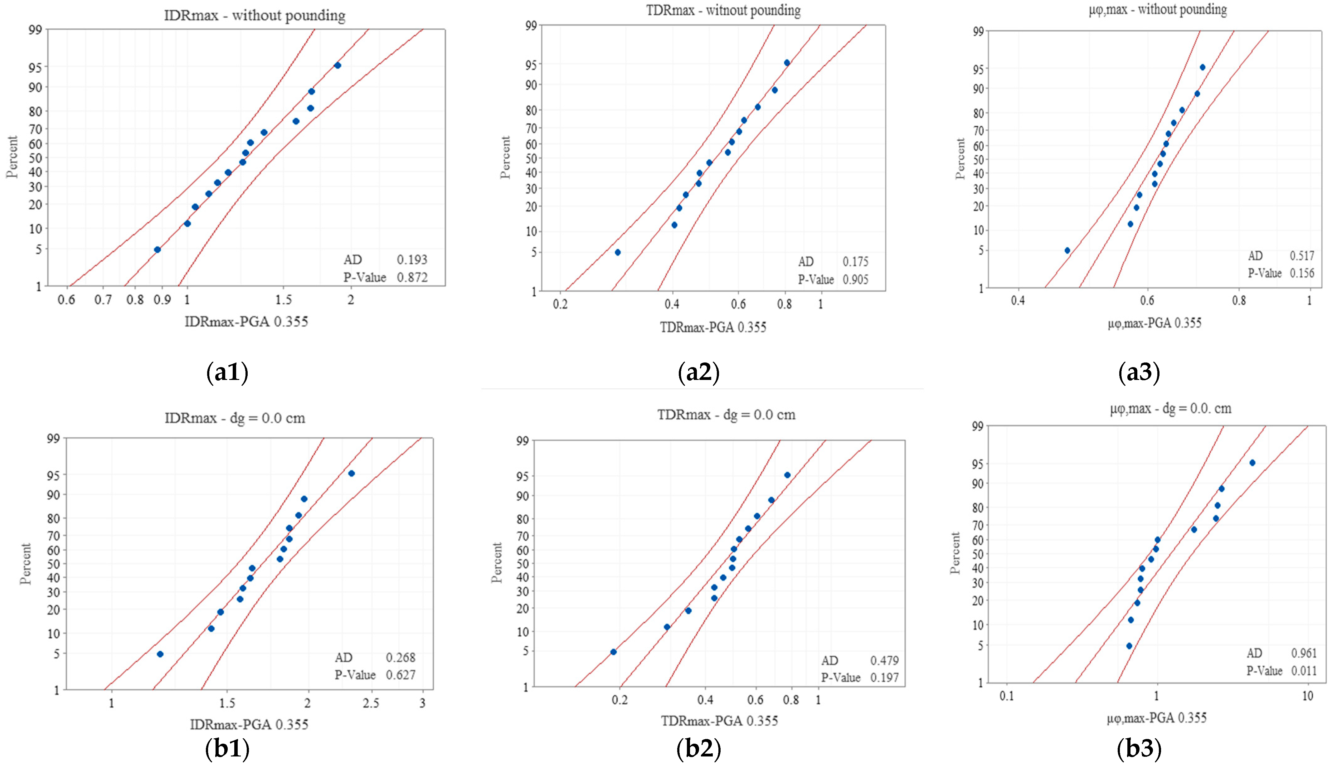
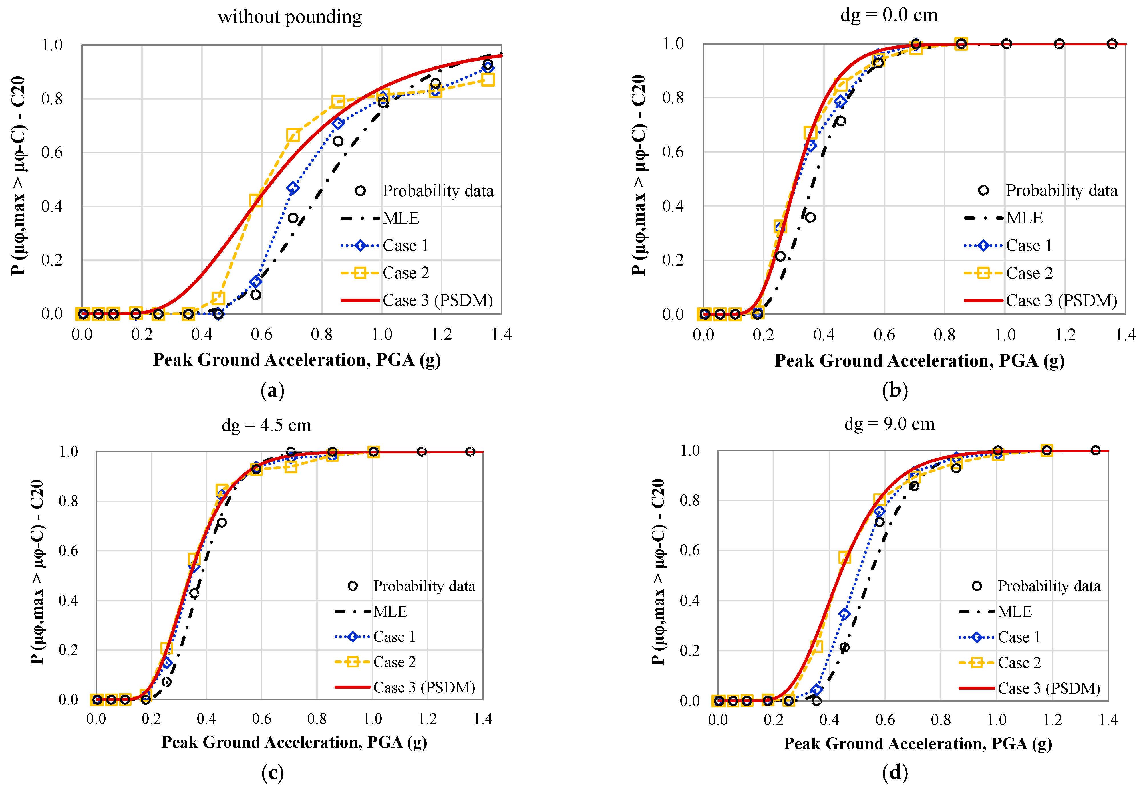
5. Validity of PSDM’s Assumptions

In this section, the validity of the assumptions that are commonly used to produce a PSDM is examined. The considered assumptions are:

i.

lognormal distribution of the evaluated structural demands,

ii.

power law model relationship between EDP and IM,

iii.

constant logarithm standard deviation of structural demands over the examined range of IM (homoscedasticity assumption).

Lognormality assumption

The validity of the lognormality assumption is examined according to the Anderson–Darling (AD) test. In general, the Anderson–Darling test measures how well the data follow a particular distribution. The smaller the AD value, the better the distribution fits to the data. Through the AD test, the p-value is calculated in order to determine which distribution fits better to data set [63].

The AD test is implemented for each level of PGA considering a confidence level equal to 95%. For each level of PGA, the implemented hypothesis test is as follows: For H_o (null hypothesis), the data follow lognormal distribution; and for H₁, the data do not follow the lognormal distribution. If the p-value for the AD test is lower than the significance level of 0.05, data do not follow lognormal distribution. On the other hand, the null hypothesis cannot be rejected. In Figure 8, indicative results of the probability plots at the level of PGA = 0.355 g are presented, while

Table 3. Check of the lognormality assumption (p-value cut off equal to 0.05).

EDPs	Examined Case	PGA (g)
		0.005	0.055	0.105	0.180	0.255	0.355	0.455	0.580	0.705	0.855	1.005	1.18	1.355
IDRmax (%hst)	without pounding	0.391	0.288	0.349	0.516	0.605	0.872	0.851	0.150	0.559	0.617	0.800	0.61	0.34
	dg = 0.0 cm	0.149	0.140	0.241	0.023	0.488	0.627	0.139	0.247	0.823	0.896	- *	- *	- *
	dg = 4.5 cm	0.398	0.403	0.232	0.785	0.769	0.511	0.411	0.871	0.234	0.843	0.138	- *	- *
	dg = 9.0 cm	0.398	0.403	0.232	0.773	0.952	0.660	0.760	0.316	0.079	0.483	0.109	0.93	- *
TDRmax (%Htot)	without pounding	0.848	0.958	0.948	0.723	0.759	0.905	0.662	0.241	0.314	0.841	0.904	0.31	0.40
	dg = 0.0 cm	0.536	0.815	0.491	0.087	0.493	0.197	0.134	0.652	0.914	0.745	- *	- *	- *
	dg = 4.5 cm	0.790	0.989	0.944	0.661	0.884	0.514	0.567	0.174	0.442	0.738	0.716	- *	- *
	dg = 9.0 cm	0.790	0.989	0.944	0.674	0.759	0.844	0.584	0.264	0.388	0.516	0.829	- *	- *
C20 μφ,max	without pounding	0.889	0.597	0.726	0.404	0.382	0.156	0.097	0.252	0.423	0.082	0.141	0.61	0.41
	dg = 0.0 cm	0.196	0.771	0.047	0.902	0.035	0.011	0.096	0.301	0.187	0.099	- *	- *	- *
	dg = 4.5 cm	0.794	0.536	0.535	0.967	0.309	0.178	0.388	0.777	0.130	0.210	0.100	- *	- *
	dg = 9.0 cm	0.794	0.536	0.535	0.777	0.249	0.037	0.010	0.042	0.098	<0.005	<0.005	- *	- *

* no available result.

shows the p-values of all the examined cases.

It can be observed that, although the assumption of the lognormal distribution cannot be rejected in the case of considering the IDR_max and TDR_max seismic demands, in the case of μ_φ,max, the distribution of the data does not match the lognormal distribution for all the examined levels of PGA (see Table 3).

Power law model

The second assumption of the PSDM concerns the relationship between the median structural demand and the intensity measure (IM). It is assumed that the mathematical relationship between $\widehat{\mathrm{EDP}}$ and IM can be approximated by a power law model and, thus, the representation of EDP-IM pairs in log-log space (lognormality assumption) implies that the structural response variates linearly (Equation (10)) with the intensity measure. Therefore, the median structural demand lies on a line at any level of IM [64]. However, linear representation of the PSDM along the range of IM is not always accurate and the adoption of a bilinear model is required to describe the variation of the structural demand especially when the components exhibit significant nonlinear behavior. In Figure 9 and Figure 10, the accuracy of using the power law model to describe the demands of IDR_max and TDR_max as a function of the PGA, is examined. In these figures, the blue dots show the structural demands retrieved based on IDAs, the black rhombus dots represent the median value of EDPs’ stripes at each level of IM, and the red lines depict the produced PSDM. Figure 9 shows that the probabilistic seismic demand model in terms of IDR_max is in good agreement with the median demand at each level of IM for all the examined cases. The same results are also yielded in the case of TDR_max. As it can be observed in Figure 10, the median TDR_max demand at each level of PGA is very close with the probabilistic seismic demand model for all the examined cases. Therefore, the linear PSDM can be used to generate the seismic demands of the eight-story frame in terms of IDR_max and TDR_max in the context of the probabilistic assessment procedure.

In Figure 11, comparative results between linear and bilinear PSDMs of the column C20 in terms of μ_φ,max|PGA are presented. These results are compared with the corresponding median demands at each level of PGA.

It can be observed that the median data are differentiated from the PSDMs in the case of using a linear regression model. These differences are more pronounced in the case where the pounding effect is evaluated, and especially when the structural members start to exhibit significant nonlinear behavior due to the interaction with the adjacent shorter and stiffer structure.

Homoscedasticity Assumption

The last assumption for the formulation of the PSDM concerns the logarithm standard deviation (${\mathsf{\beta }}_{\mathrm{EDP}|\mathrm{IM}}$) of the demand. In order to evaluate the validity of homoscedasticity assumption, the area limited between the mean plus and minus one standard deviation of the associated normal distribution at each level of IM is defined. So, in Figure 9, Figure 10 and Figure 11, the green shaded area shows the variation of the demands along the examined range of PGA. Figure 9 shows that the variation of demands in terms of the IDR_max is not constant but is slightly reduced for values of PGA greater than 0.255 g. Similar results are also deduced in the case of TDR_max, as it can be observed in Figure 10.

Therefore, the homoscedasticity assumption of producing the PSDM of IDR_max and TDR_max is not satisfied within the overall range of PGA. Furthermore, the interaction between the adjacent structures has not altered the outcomes related to the homoscedasticity assumption of the PSDM in terms of displacement EDPs. On the contrary, the case of structural pounding between adjacent structures has altered the outcomes related to the homoscedasticity of the PSDM in terms of μ_φ,max|PGA. As it is discussed below, this is attributed to the effect of pounding on the local inelastic demands of the column.

Results of Figure 11 clearly indicate that the linear PSDM cannot adequately describe the maximum local curvature ductility demands, i.e., μ_φ,max of the critical column, due to the pounding effect (Figure 11a). For the bilinear PSDMs, the validity of the homoscedasticity assumption is evaluated at each linear branch of the regression model. Small fluctuations in the dispersion along the first branch of the regression model are observed, and the response of the column is still an elastic one. On the other hand, the nonlinear behavior of the structural member results in a large variation of the demands that differs significantly for each ground motion. These variations are depicted at the second branch of the PSDM.

Thus, it could be pointed out that the nonlinear local demands of the structural member are not sufficiently reflected on the homoscedasticity assumption when only linear PSDM is adopted.

Interaction of Assumptions on Developing Fragility Curves

In this part of the study, the influence of the PSDM assumptions on the fragility curves is examined in order to provide a better insight of the bias induced. For this purpose, the following three different hypothesis cases are considered:

• Case 1 (lognormality assumption)
  In this case, only the lognormality assumption is considered for developing the fragility curves. So, the value of the probability is defined accounting the mean and the standard deviation of each distribution at a particular level of IM.
• Case 2 (lognormality assumption and power law model)
  The lognormality assumption is considered in combination with the power law model. The median of the structural demand at a particular level of IM is based on the PSDM, while the dispersion is calculated for each level of IM through Equation (11).
• Case 3 (lognormality assumption, power law model, and homoscedasticity assumption)
  The three basic assumptions of PSDM are considered for the development of the fragility curves.

The available separation gap distances d_g between the adjacent structures and the case of without pounding effect are also incorporated. Furthermore, the discrete probability data points (empirical CDF method) and the MLE-based fragility curve (as a reliable continuous fragility curve) are used for the quantification of the bias induced through assumptions.

In Figure 12 and Figure 13, the fragility curves in terms of IDR_max|PGA and TDR_max|PGA based on the examined hypothesis cases (1–3) are presented. As observed, the examined fragility curves are in a good agreement with the assessment based on the MLE method. Therefore, the violation of the homoscedasticity assumption for both EDPs does not influence the fragility assessment of the pounding effect. So, PSDMs for both EDPs are sufficient estimators of the structural demand on the fragility assessment of the eight-story RC frame structure subjected to pounding.

In Figure 14, the corresponding fragility curves that are produced considering the three different hypothesis cases in terms of μ_φ,max|PGA at the performance level of DL, are presented. It is observed that the fragility curves are significantly influenced by the assumptions made on the formulation of PSDMs when the seismic performance of eight-story frame is evaluated without considering the pounding between the adjacent structure (Figure 14a). The error induced due to the power law model and the homoscedasticity assumption in the case of μ_φ,max seems to be considerably high. However, this outcome is not so intense when the effect of structural pounding is assessed. This is attributed to the use of bilinear PSDM to describe the critical inelastic behavior of the column at low levels of IM (Figure 14b–d).

6. Conclusions

In this study, five different methodologies for developing fragility curves are evaluated to assess the seismic performance of real RC structures subjected to structural pounding. For this purpose, the discrete probability data points deduced based on the empirical CDF method are utilized to validate the fragility curves developed through MLE, MM, IM percentiles, and PSDM procedures. Displacement-based and curvature-based fragility curves are developed. The use of probabilistic seismic demand models on the fragility assessment of the pounding risk is further estimated. Linear and bilinear PSDMs are developed, while the validity of the assumptions commonly used to produce a PSDM is examined. Finally, the influence of the PSDMs’ assumptions on the derivation of the fragilities for the structural pounding effect is identified. The examined structural pounding cases are between an eight-story RC frame and a three-story rigid structure that have equal story heights (floor-to-floor interaction). The main outcomes of this study are as follows:

• The MLE, MM, and IM percentiles procedures are developing fragilities that are in a good agreement with the probability data points of the empirical CDF method.
• The IM percentiles method gives more conservative results in terms of TDR_max|PGA, in comparison to the other methodologies of this study. Nevertheless, in the case of μ_φ,max|PGA, the fragility curve is moved towards greater values of PGA when d_g = 0.0 cm. This result indicates that the IM-percentiles-based local fragility curve cannot accurate capture the increased inelastic demands of the column due to the pounding effect, when d_g = 0.0 cm.
• The displacement-based fragilities that are developing from the PSDMs are shifted to greater values of PGA in comparison to the deduced fragilities based on the MLE, MM, and IM percentiles procedures.
• The curvature-based fragilities that are developing from the PSDMs are shifted to lower values of PGA in comparison to the deduced fragilities based on the MLE, MM, and IM percentiles procedures.
• Similar results regarding the fragility assessment of the RC structure between the examined methodologies are deduced when the performance level controls the seismic behavior of the eight-story RC frame structure at low levels of IM.
• The observed shift on the fragility curves is owed to the different values of medians μ that methodologies estimate.
• The lognormality assumption that is evaluated for each level of PGA showing that it is not always satisfied especially in the case of maximum curvature ductility.
• The homoscedasticity assumption of developing the PSDM of IDR_max and TDR_max is not satisfied within the overall range of PGA.
• The use of a linear PSDM fails to properly describe the local inelastic demands of the structural RC member.
• The nonlinear local demands of the structural member are not sufficiently reflected on the homoscedasticity assumption when only linear PSDM is adopted. The errors induced due to the power law model and the homoscedasticity assumptions of the PSDM can be reduced by using a bilinear regression model.

References

1. Whitman, R.V.; Biggs, J.M.; Brennan, J.E.; Cornell, C.A.; De Neufville, R.L.; Vanmarcke, E.H. Seismic Design Decision Analysis. J. Struct. Div. 1975, 101, 1067–1084. [Google Scholar] [CrossRef]
2. Applied Technology Council (ATC). Seismic Vulnerability and Impact of Disruption of Lifelines in the Conterminous United States; Report No. ATC-25; ATC: Redwood City, CA, USA, 1991. [Google Scholar]
3. Schneider, P.J.; Schauer, B.A. HAZUS—Its Development and Its Future. Nat. Hazards Rev. 2006, 7, 40–44. [Google Scholar] [CrossRef]
4. Mackie, K.; Stojadinovic, B. Fragility Basis for California Highway Overpass Bridge Seismic Decision Making; PEER 2005/12; University of California: Berkeley, CA, USA, 2005. [Google Scholar]
5. Applied Technology Council (ATC). Earthquake Damage Evaluation Data for California; Report No. ATC-13; ATC: Redwood City, CA, USA, 1985. [Google Scholar]
6. Kostov, M.; Kaneva, A.; Vaseva, M.; Stefanov, D.; Koleva, N. An Advanced spproach to earthquake risk scenarios of Sofia. In Proceedings of the 8th Pacific Conference on Earthquake Engineering, Singapore, Australia, 5–7 December 2007; pp. 1–9. [Google Scholar]
7. Rossetto, T.; Elnashai, A. Derivation of vulnerability functions for European-type RC structures based on observational data. Eng. Struct. 2003, 25, 1241–1263. [Google Scholar] [CrossRef]
8. Basöz, N.; Kiremidjian, A.S. Evaluation of Bridge Damage Data from the Loma Prieta and Northridge CA Earthquakes; Report No. MCEER-98-0004; University at Buffalo: Buffalo, NY, USA, 1997. [Google Scholar]
9. Sarabandi, P.; Pachakis, D.; King, S. Empirical fragility functions from recent earthquakes. In Proceedings of the 13th World Conference on Earthquake Engineering, Vancouver, BC, Canada, 1–6 August 2004; pp. 1–15. [Google Scholar]
10. Rota, M.; Penna, A.; Strobbia, C.; Magenes, G. Direct derivation of fragility curves from Italian post-earthquake survey data. In Proceedings of the 14th World Conference on Earthquake Engineering, Beijing, China, 12–17 October 2008; pp. 1–8. [Google Scholar]
11. Colombi, M.; Borzi, B.; Crowley, H.; Onida, M.; Meroni, F.; Pinho, R. Deriving vulnerability curves using Italian earthquake damage data. Bull. Earthq. Eng. 2008, 6, 485–504. [Google Scholar] [CrossRef]
12. Vosooghi, A.; Saiidi, M.S. Experimental Fragility Curves for Seismic Response of Reinforced Concrete Bridge Columns. ACI Struct. J. 2012, 109, 825–834. [Google Scholar] [CrossRef]
13. Mander, J.B.; Basöz, N. Seismic fragility curves theory for highway bridges. In Proceedings of the 5th US Conference on Lifeline Earthquake Engineering: Optimazing Post-Earthquake Lifeline System Reliability, Seattle, WA, USA, 12–14 August 1999; pp. 31–40. [Google Scholar]
14. Moschonas, I.F.; Kappos, A.J.; Panetsos, P.; Papadopoulos, V.; Makarios, T.; Thanopoulos, P. Seismic fragility curves for greek bridges: Methodology and case studies. Bull. Earthq. Eng. 2008, 7, 439–468. [Google Scholar] [CrossRef]
15. Shinozuka, M.; Feng, M.Q.; Kim, H.-K.; Kim, S.-H. Nonlinear Static Procedure for Fragility Curve Development. J. Eng. Mech. 2000, 126, 1287–1295. [Google Scholar] [CrossRef] [Green Version]
16. Karim, K.R.; Yamazaki, F. A simplified method of constructing fragility curves for highway bridges. Earthq. Eng. Struct. Dyn. 2003, 32, 1603–1626. [Google Scholar] [CrossRef]
17. Kwon, O.-S.; Elnashai, A.S. Fragility analysis of a highway over-crossing bridge with consideration of soil–structure interactions. Struct. Infrastruct. Eng. 2010, 6, 159–178. [Google Scholar] [CrossRef]
18. Nielson, B.G.; Desroches, R. Analytical Seismic Fragility Curves for Typical Bridges in the Central and Southeastern United States. Earthq. Spectra 2007, 23, 615–633. [Google Scholar] [CrossRef]
19. Nielson, B.G.; Desroches, R. Seismic fragility methodology for highway bridges using a component level approach. Earthq. Eng. Struct. Dyn. 2007, 36, 823–839. [Google Scholar] [CrossRef]
20. Padgett, J.E. Seismic Vulnerability Assessment of Retrofitted Bridges Using Probabilistic Methods. Ph.D. Thesis, Georgia Institute of Technology, Atlanta, GA, USA, 4 April 2007. [Google Scholar]
21. Mosleh, A.; Razzaghi, M.S.; Jara, J.; Varum, H. Seismic fragility analysis of typical pre-1990 bridges due to near- and far-field ground motions. Int. J. Adv. Struct. Eng. 2016, 8, 1–9. [Google Scholar] [CrossRef] [Green Version]
22. Mosleh, A.; Razzaghi, M.S.; Jara, J.; Varum, H. Development of fragility curves for RC bridges subjected to reverse and strike-slip seismic sources. Earthquakes Struct. 2016, 11, 517–538. [Google Scholar] [CrossRef] [Green Version]
23. Mosleh, A.; Jara, J.; Razzaghi, M.S.; Varum, H. Probabilistic Seismic Performance Analysis of RC Bridges. J. Earthq. Eng. 2018, 24, 1704–1728. [Google Scholar] [CrossRef]
24. Erberik, M.; Elnashai, A.S. Fragility analysis of flat-slab structures. Eng. Struct. 2004, 26, 937–948. [Google Scholar] [CrossRef]
25. Kirçil, M.S.; Polat, Z. Fragility analysis of mid-rise R/C frame buildings. Eng. Struct. 2006, 28, 1335–1345. [Google Scholar] [CrossRef]
26. Hwang, H.; Jernigan, J.B.; Lin, Y.-W. Evaluation of Seismic Damage to Memphis Bridges and Highway Systems. J. Bridg. Eng. 2000, 5, 322–330. [Google Scholar] [CrossRef]
27. Yu, O.; Allen, D.L.; Drnevich, V.P. Seismic vulnerability assessment of bridges on earthquake priority routes in Western Kentucky. Proceedings of 3rd US National Conference on Lifeline Earthquake Engineering, Los Angeles, CA, USA, 22–23 August 1991; pp. 817–826. [Google Scholar]
28. Kappos, A.J.; Pitilakis, K.; Stylianidis, K.C. Cost-Benefit analysis for the seismic rehabilitation of buildings in Thessaloniki, based on a hybrid method of vulnerability assessment. In Proceedings of the Fifth International Conference on Seismic Zonation, Nice, France, 17–19 October 1995; pp. 406–413. [Google Scholar]
29. Kappos, A.J.; Stylianidis, K.C.; Pitilakis, K. Development of Seismic Risk Scenarios Based on a Hybrid Method of Vulnerability Assessment. Nat. Hazards 1998, 17, 177–192. [Google Scholar] [CrossRef]
30. Kappos, A.J.; Panagopoulos, G.; Panagiotopoulos, C.; Penelis, G. A hybrid method for the vulnerability assessment of R/C and URM buildings. Bull. Earthq. Eng. 2006, 4, 391–413. [Google Scholar] [CrossRef]
31. Cornell, C.A.; Jalayer, F.; Hamburger, R.O.; Foutch, D.A. Probabilistic Basis for 2000 SAC Federal Emergency Management Agency Steel Moment Frame Guidelines. J. Struct. Eng. 2002, 128, 526–533. [Google Scholar] [CrossRef] [Green Version]
32. Bazzurro, P.; Cornell, C.A.; Shome, N.; Carballo, J.E. Three Proposals for Characterizing MDOF Nonlinear Seismic Response. J. Struct. Eng. 1998, 124, 1281–1289. [Google Scholar] [CrossRef]
33. Shome, N.; Cornell, C.A.; Bazzurro, P.; Carballo, J.E. Earthquakes, Records, and Nonlinear Responses. Earthq. Spectra 1998, 14, 469–500. [Google Scholar] [CrossRef]
34. Vamvatsikos, D.; Cornell, C.A. Incremental dynamic analysis. Earthq. Eng. Struct. Dyn. 2002, 31, 491–514. [Google Scholar] [CrossRef]
35. Jalayer, F.; Cornell, C.A. A Technical Framework for Probability-Based Demand and Capacity Factor Design (DCFD) Seismic Formats; PEER 2003/08; University of California: Berkeley, CA, USA, 2003. [Google Scholar]
36. Jalayer, F.; Cornell, C.A. Alternative non-linear demand estimation methods for probability-based seismic assessments. Earthq. Eng. Struct. Dyn. 2009, 38, 951–972. [Google Scholar] [CrossRef]
37. Porter, K.; Kennedy, R.; Bachman, R. Creating Fragility Functions for Performance-Based Earthquake Engineering. Earthq. Spectra 2007, 23, 471–489. [Google Scholar] [CrossRef]
38. Baker, J.W. Fitting Fragility Functions to Structural Analysis Data Using Maximum Likelihood Estimation. Working Paper–PEER. 2011. Available online: https://www.scirp.org/(S(vtj3fa45qm1ean45vvffcz55))/reference/ReferencesPapers.aspx?ReferenceID=1344212 (accessed on 1 August 2021).
39. Bakalis, K.; Vamvatsikos, D. Seismic Fragility Functions via Nonlinear Response History Analysis. J. Struct. Eng. 2018, 144, 04018181. [Google Scholar] [CrossRef]
40. Tubaldi, E.; Freddi, F.; Barbato, M. Probabilistic seismic demand model for pounding risk assessment. Earthq. Eng. Struct. Dyn. 2016, 45, 1743–1758. [Google Scholar] [CrossRef]
41. Ramamoorthy, S.K.; Gardoni, P.; Bracci, J.M. Probabilistic Demand Models and Fragility Curves for Reinforced Concrete Frames. J. Struct. Eng. 2006, 132, 1563–1572. [Google Scholar] [CrossRef]
42. Bai, J.-W.; Gardoni, P.; Hueste, M.B.D. Story-specific demand models and seismic fragility estimates for multi-story buildings. Struct. Saf. 2011, 33, 96–107. [Google Scholar] [CrossRef]
43. Freddi, F.; Padgett, J.E.; Dall’Asta, A. Probabilistic seismic demand modeling of local level response parameters of an RC frame. Bull. Earthq. Eng. 2016, 15, 1–23. [Google Scholar] [CrossRef]
44. Aljawhari, K.; Gentile, R.; Freddi, F.; Galasso, C. Effects of ground-motion sequences on fragility and vulnerability of case-study reinforced concrete frames. Bull. Earthq. Eng. 2020, 1–31. [Google Scholar] [CrossRef]
45. Gardoni, P.; Der Kiureghian, A.; Mosalam, K.M. Probabilistic Capacity Models and Fragility Estimates for Reinforced Concrete Columns based on Experimental Observations. J. Eng. Mech. 2002, 128, 1024–1038. [Google Scholar] [CrossRef]
46. Gardoni, P.; Mosalam, K.M.; Der Kiureghian, A. Probabilistic seismic demand models and fragility estimates for rc bridges. J. Earthq. Eng. 2003, 7, 79–106. [Google Scholar] [CrossRef]
47. Jalayer, F.; Ebrahimian, H.; Miano, A.; Manfredi, G.; Sezen, H. Analytical fragility assessment using unscaled ground motion records. Earthq. Eng. Struct. Dyn. 2017, 46, 2639–2663. [Google Scholar] [CrossRef]
48. Nazri, F.M.; Miari, M.; Kassem, M.M.; Tan, C.-G.; Farsangi, E.N. Probabilistic Evaluation of Structural Pounding Between Adjacent Buildings Subjected to Repeated Seismic Excitations. Arab. J. Sci. Eng. 2018, 44, 4931–4945. [Google Scholar] [CrossRef]
49. Flegga, M.; Favvata, M. Global and local performance levels on the probabilistic evaluation of the structural pounding effect between adjacent rc structures. In Proceedings of the 11 International Conference on Structural Dynamics, EURODYN, Athens, Greece, 23–26 November 2020; pp. 3762–3779. [Google Scholar] [CrossRef]
50. Kazemi, F.; Miari, M.; Jankowski, R. Investigating the effects of structural pounding on the seismic performance of adjacent RC and steel MRFs. Bull. Earthq. Eng. 2020, 19, 317–343. [Google Scholar] [CrossRef]
51. Flenga, M.G.; Favvata, M.J. Probabilistic seismic assessment of the pounding risk based on the local demands of a multistory RC frame structure. Eng. Struct. 2021, 245, 112789. [Google Scholar] [CrossRef]
52. Aslani, H.; Miranda, E. Fragility assessment of slab-column connections in existing non-ductile reinforced concrete buildings. J. Earthq. Eng. 2005, 9, 777–804. [Google Scholar] [CrossRef]
53. Freddi, F.; Tubaldi, E.; Ragni, L.; Dall’Asta, A. Probabilistic performance assessment of low-ductility reinforced concrete frames retrofitted with dissipative braces. Earthq. Eng. Struct. Dyn. 2012, 42, 993–1011. [Google Scholar] [CrossRef]
54. Mackie, K.R.; Stojadinović, B. Comparison of Incremental Dynamic, Cloud, and Stripe Methods for Computing Probabilistic Seismic Demand Models. In Proceedings of the Structures Congress 2005: Metropolis and Beyond, New York, NY, USA, 20–24 April 2005; pp. 1–11. [Google Scholar] [CrossRef]
55. Shome, N. Probabilistic Seismic Demand Analysis of Nonlinear Structures; Report No. RMS-35; Department of Civil Engineering, Stanford University: Stanford, CA, USA, 1999. [Google Scholar]
56. Prakash, V.; Powell, G.H.; Gampbell, S. DRAIN-2DX Base Program Description and User’s Guide, UCB/SEMM; Report No. 17/93; University of California: Orkland, CA, USA, 1993. [Google Scholar]
57. Karayannis, C.G.; Favvata, M.J. Inter-story pounding between multistory reinforced concrete structures. Struct. Eng. Mech. 2005, 20, 505–526. [Google Scholar] [CrossRef]
58. Karayannis, C.G.; Favvata, M.J. Earthquake-induced interaction between adjacent reinforced concrete structures with non-equal heights. Earthq. Eng. Struct. Dyn. 2004, 34, 1–20. [Google Scholar] [CrossRef]
59. Favvata, M.J. Minimum required separation gap for adjacent RC frames with potential inter-story seismic pounding. Eng. Struct. 2017, 152, 643–659. [Google Scholar] [CrossRef]
60. PEER Ground Motion Database. 2011. Available online: https://peer.berkeley.edu/peer-strong-ground-motion-databases (accessed on 10 February 2017).
61. Eurocode 8. Design of Structures for Earthquake Resistance. Part 1: General Rules, Seismic Actions and Rules for Buildings; EN 1998-1; European Committee for Standardization: Brussels, Belgium, 2004. [Google Scholar]
62. Applied Technology Council (ATC). Seismic Evaluation and Retrofit of Concrete Buildings; Report No. ATC-40; ATC: Redwood City, CA, USA, 1996; Volume 1. [Google Scholar]
63. Minitab. Available online: https://support.minitab.com (accessed on 12 May 2021).
64. Karamlou, A.; Bocchini, P.; Bochini, P. Computation of bridge seismic fragility by large-scale simulation for probabilistic resilience analysis. Earthq. Eng. Struct. Dyn. 2015, 44, 1959–1978. [Google Scholar] [CrossRef]
Figure 1. (a) Set of IDA curves and stripes of EDP at discrete values of IM, (b) Fragility curve based on empirical cumulative distribution function (CDF).
Applsci 11 08253 g001
Figure 2. Set of IDAs curves and corresponding values of IM at the level of capacity C ^ .
Applsci 11 08253 g002
Figure 3. 16%, 50%, 84% summarized IDAs curves and corresponding values of IM at the level of capacity C ^ .
Applsci 11 08253 g003
Figure 4. (a) Eight-story RC frame and (b) idealization of the contact area.
Applsci 11 08253 g004
Figure 5. MLE, MM, IM percentiles, PSDM methodologies for the fragility assessment of the eight-story RC frame in terms of maximum interstory drift (IDRmax -%hst) as a function of the PGA. Examined cases: (a) without the pounding effect, (b) dg = 0.0 cm, (c) dg = 4.5 cm, and (d) dg = 9.0 cm.
Applsci 11 08253 g005
Figure 6. MLE, MM, IM percentiles, PSDM methodologies for the fragility assessment of the eight-story RC frame in terms of maximum top drift (TDRmax -%Htot) as a function of the PGA. Examined cases: (a) without the pounding effect, (b) dg = 0.0 cm, (c) dg = 4.5 cm, and (d) dg = 9.0 cm.
Applsci 11 08253 g006
Figure 7. MLE, MM, IM percentiles, PSDM methodologies on the fragility assessment of the eight-story RC frame in terms of maximum curvature ductility μφ,max as a function of the PGA. Examined cases: (a) without the pounding effect, (b) dg = 0.0 cm, (c) dg = 4.5 cm, and (d) dg = 9.0 cm.
Applsci 11 08253 g007
Figure 8. Lognormality assumption: Probability plot at PGA = 0.355 g in the case of (a) without the pounding effect, and (b) when dg = 0.0 cm. Examined engineering demand parameters: (1) IDRmax, (2) TDRmax, and (3) μφ,max.
Applsci 11 08253 g008
Figure 9. Comparative results in terms of IDRmax (%hst) at each level of PGA as deduced based on IDAs, PSDMs, and median values of demand. Examined cases: (a) without the pounding effect, (b) dg = 0.0 cm, (c) dg = 4.5 cm, and (d) dg = 9.0 cm.
Applsci 11 08253 g009
Figure 10. Comparative results in terms of TDRmax (%Htot) at each level of PGA as deduced based on IDAs, PSDMs, and median values of demand. Examined cases: (a) without the pounding effect, (b) dg = 0.0 cm, (c) dg = 4.5 cm, and (d) dg = 9.0 cm.
Applsci 11 08253 g010
Figure 11. Comparative results in terms of μφ,max (column C20) at each level of PGA as deduced based on IDAs, PSDMs, and median values of demand. Regression models: (a) linear, and (b) bilinear. Examined cases: (1) without the pounding effect, (2) dg = 0.0 cm, (3) dg = 4.5 cm, and (4) dg = 9.0 cm.
Applsci 11 08253 g011aApplsci 11 08253 g011b
Figure 12. Influence of the PSDM assumptions on the fragility assessment of the eight-story RC frame in terms of IDRmax (%hst) as a function of the PGA. Examined assumptions: Case 1—lognormality, Case 2—lognormality and power law model, and Case 3—SDM’s assumptions. Fragility curves (a) without the pounding effect, (b) dg = 0.0 cm, (c) dg = 4.5 cm, and (d) dg = 9.0 cm.
Applsci 11 08253 g012
Figure 13. Influence of the PSDM assumptions on the fragility assessment of the eight-story RC frame in terms of TDRmax (%Htot) as a function of the PGA. Examined assumptions: Case 1—lognormality, Case 2—lognormality and power law model, Case 3—PSDM’s assumptions. Fragility curves (a) without the pounding effect, (b) dg = 0.0 cm, (c) dg = 4.5 cm, and (d) dg = 9.0 cm.
Applsci 11 08253 g013aApplsci 11 08253 g013b
Figure 14. Influence of the PSDM assumptions on the fragility assessment of the eight-story RC frame in terms of μφ,max (C20) as a function of the PGA. Examined assumptions: Case 1—lognormality, Case 2—lognormality and power law model, Case 3—PSDM’s assumptions. Fragility curves (a) without the pounding effect, (b) dg = 0.0 cm, (c) dg = 4.5 cm, and (d) dg = 9.0 cm.
Applsci 11 08253 g014