
Monitoring of Heavy Metals and Nitrogen Concentrations in Mosses in the Vicinity of an Integrated Iron and Steel Plant: Case Study in Czechia


Abstract
:Featured Application
Abstract
1. Introduction
2. Experiments
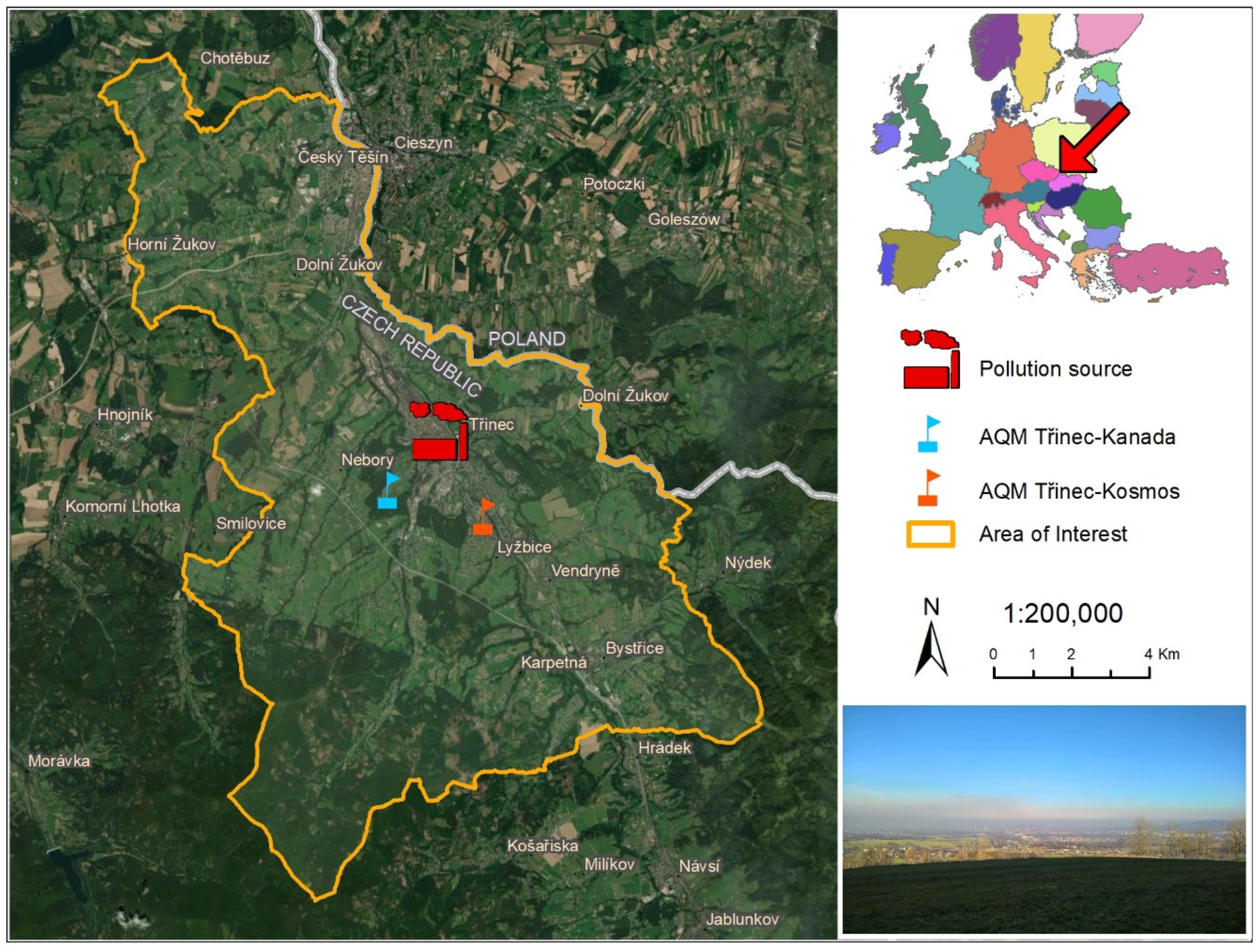
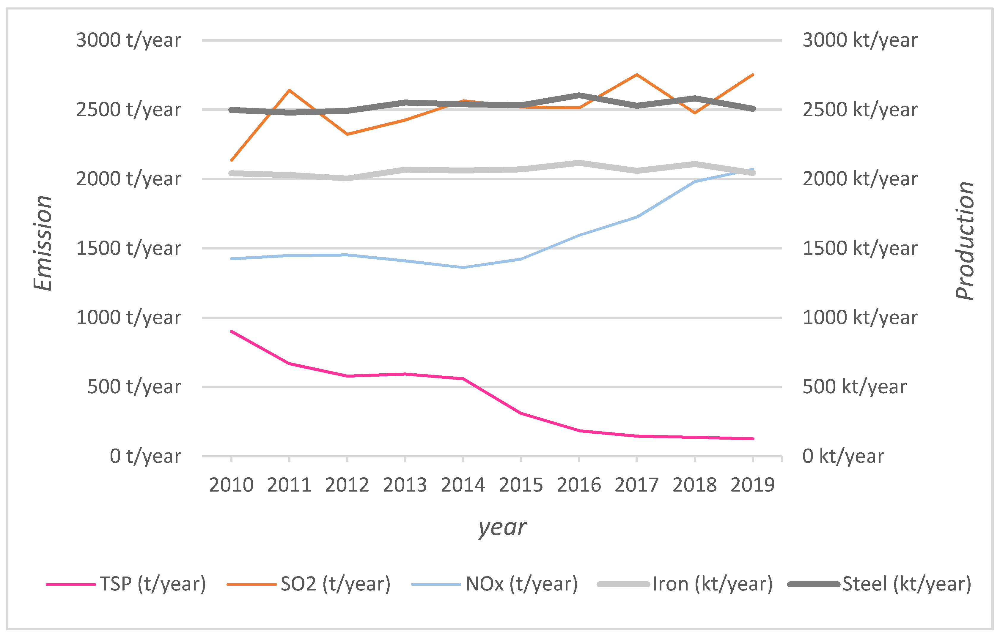
2.1. Study Area
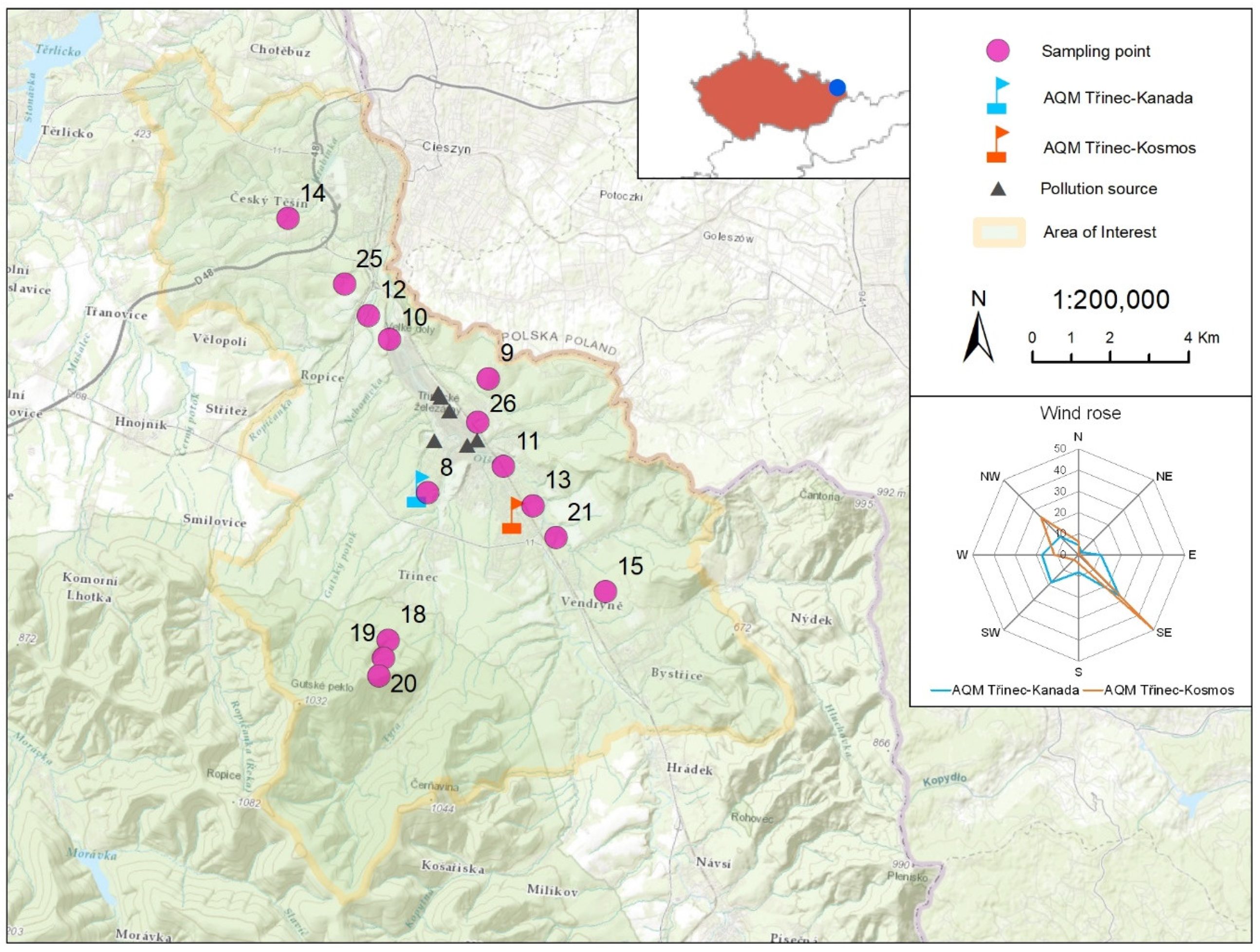
2.2. Sampling
2.3. Sample Analyses
2.4. Statistical Analyses and Visualisation
2.5. Modelling of PM Concentrations
3. Results
3.1. Elements Content
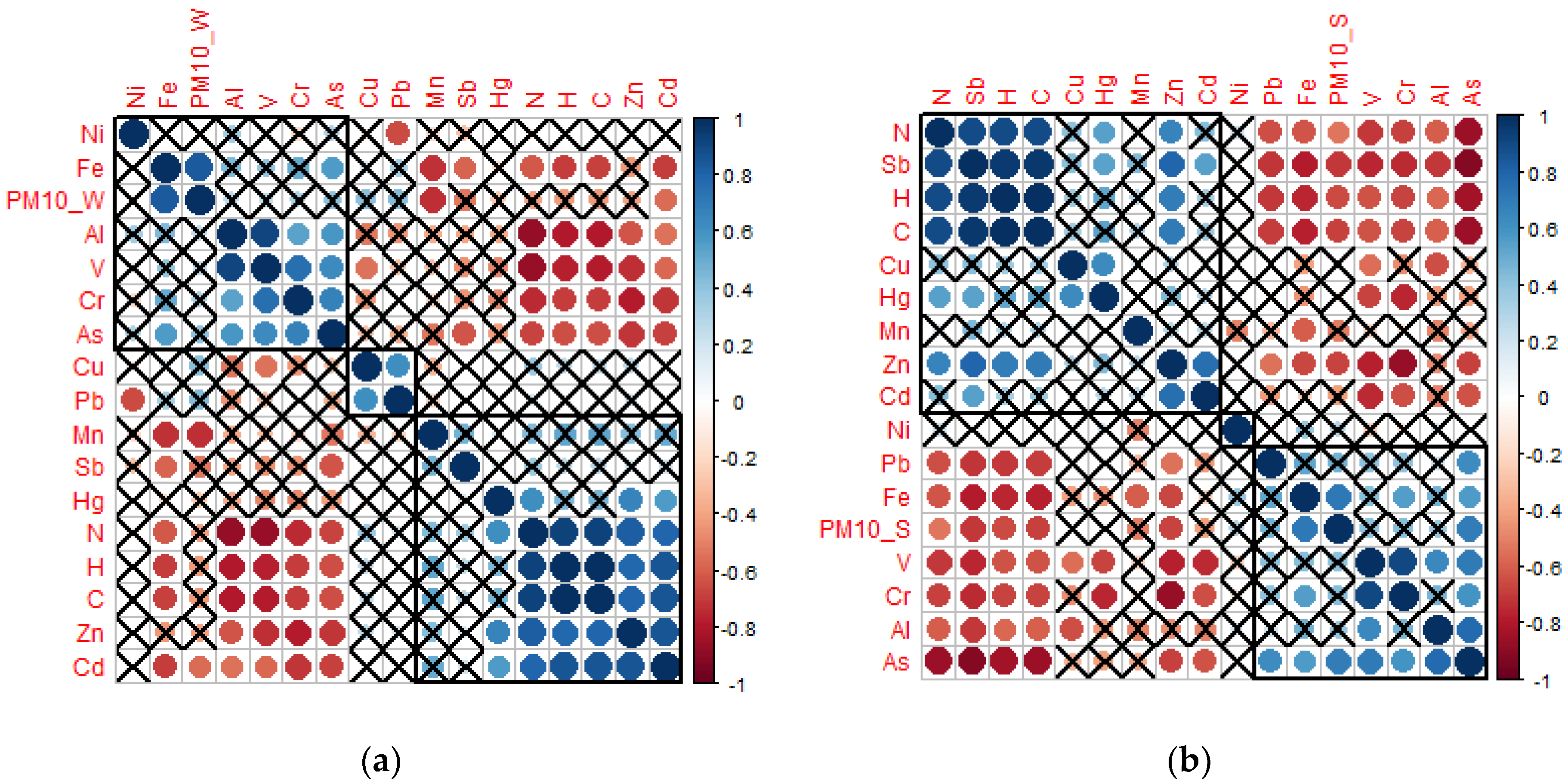
3.2. Elements Correlations
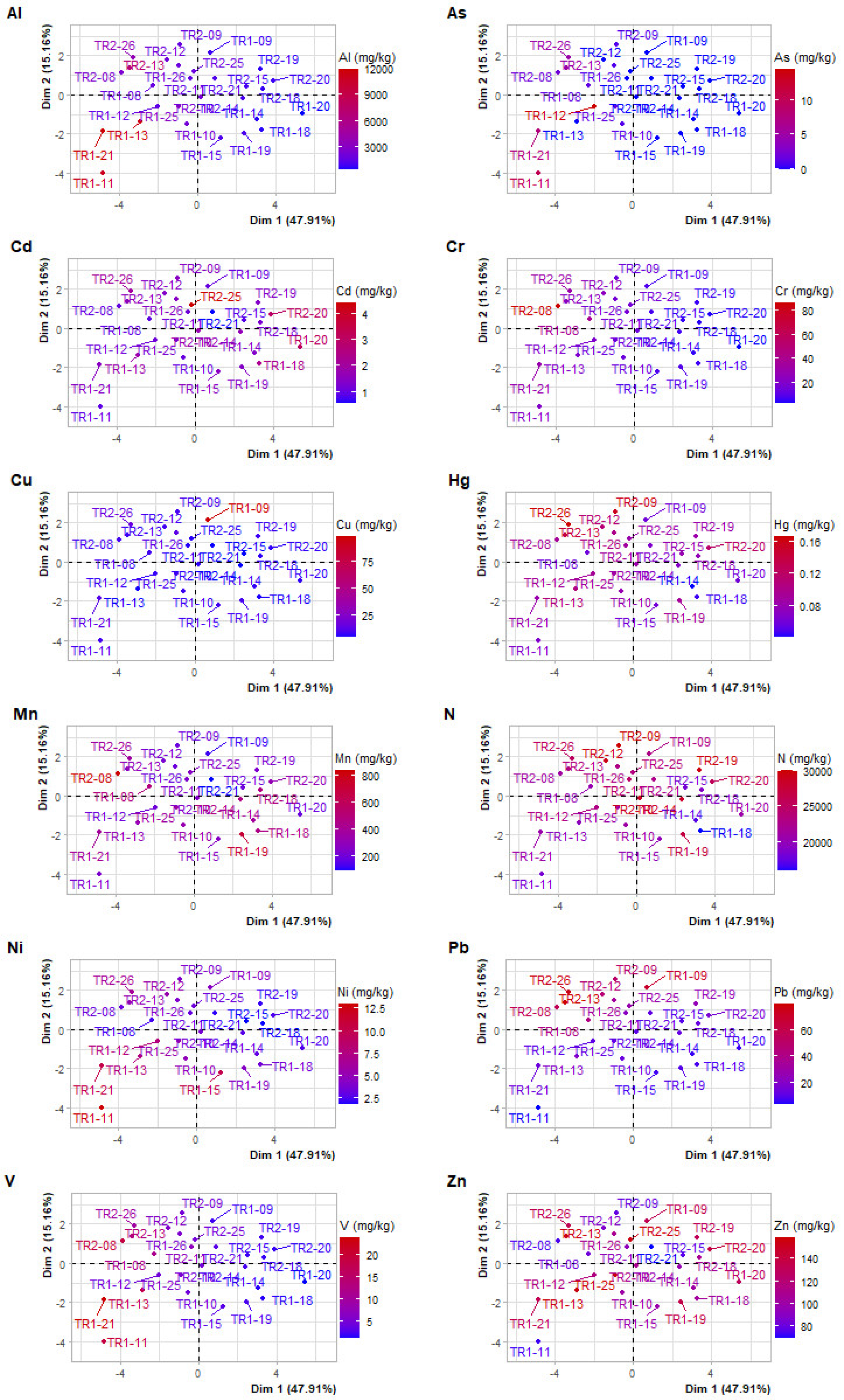
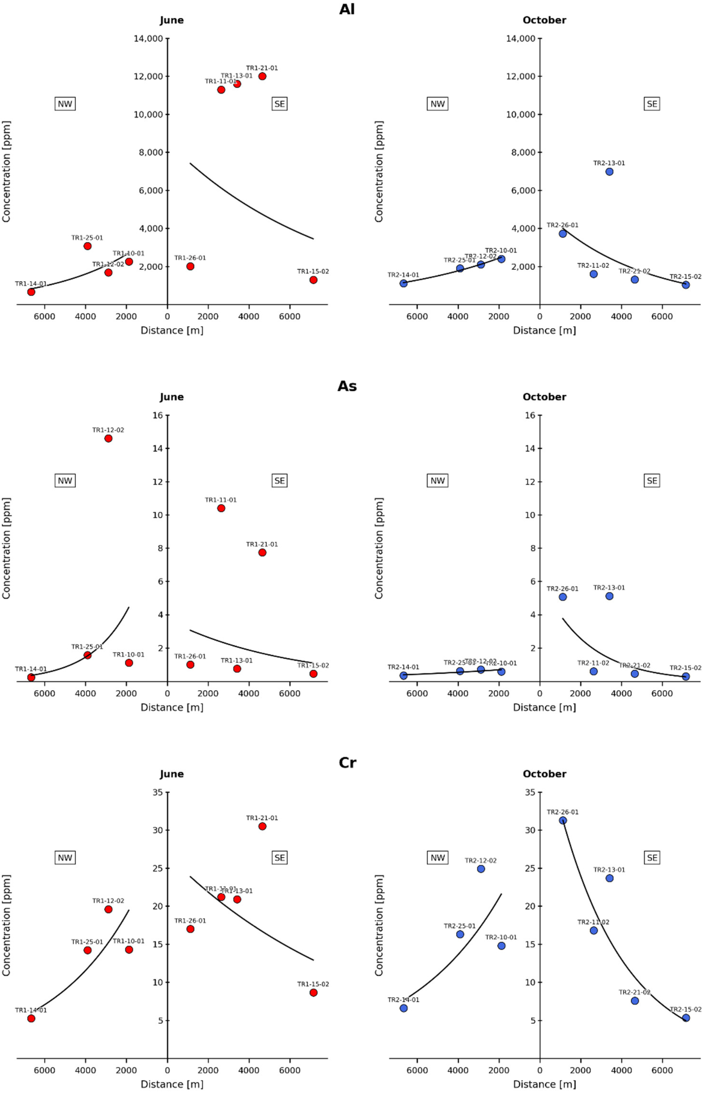
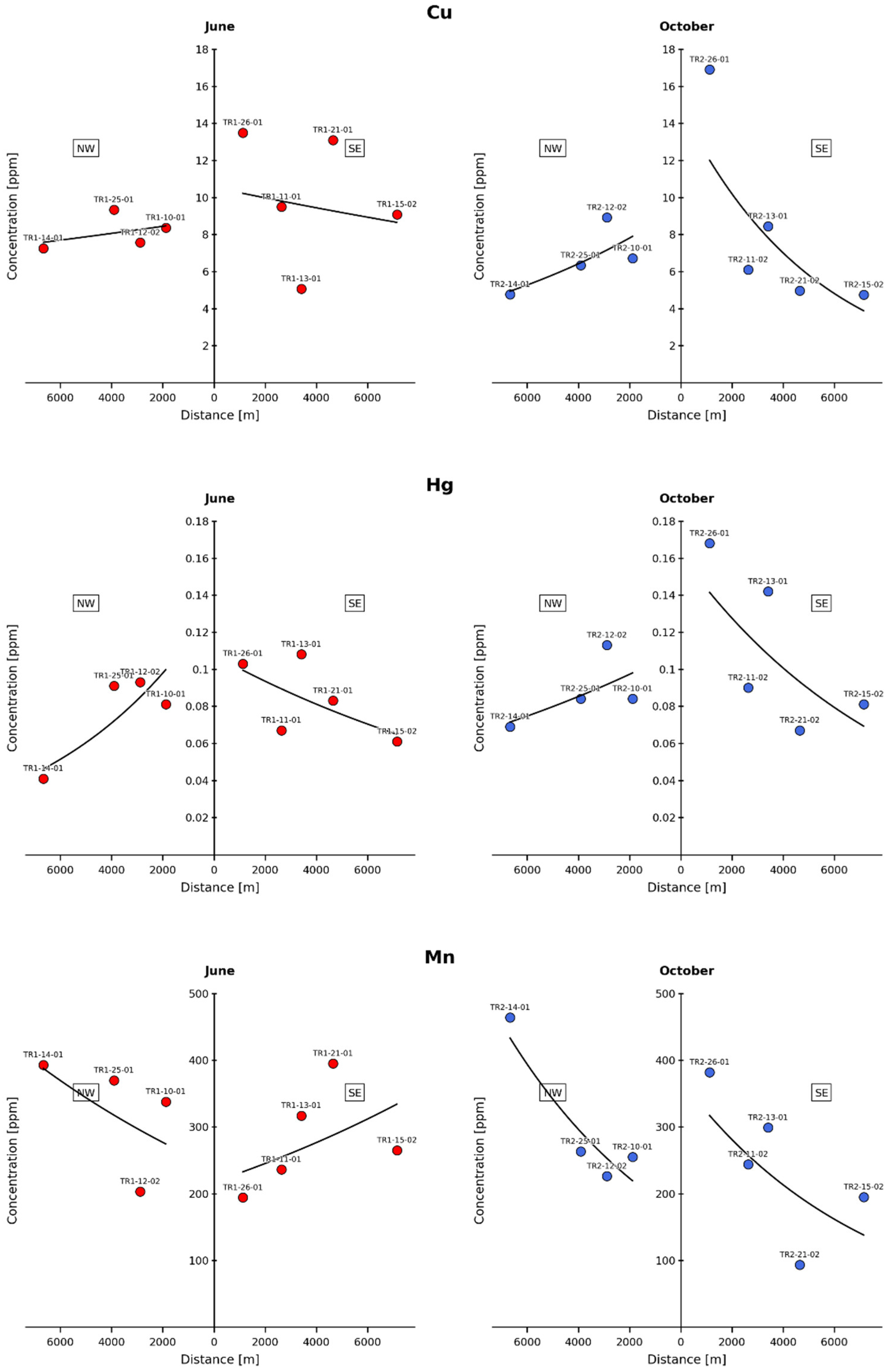
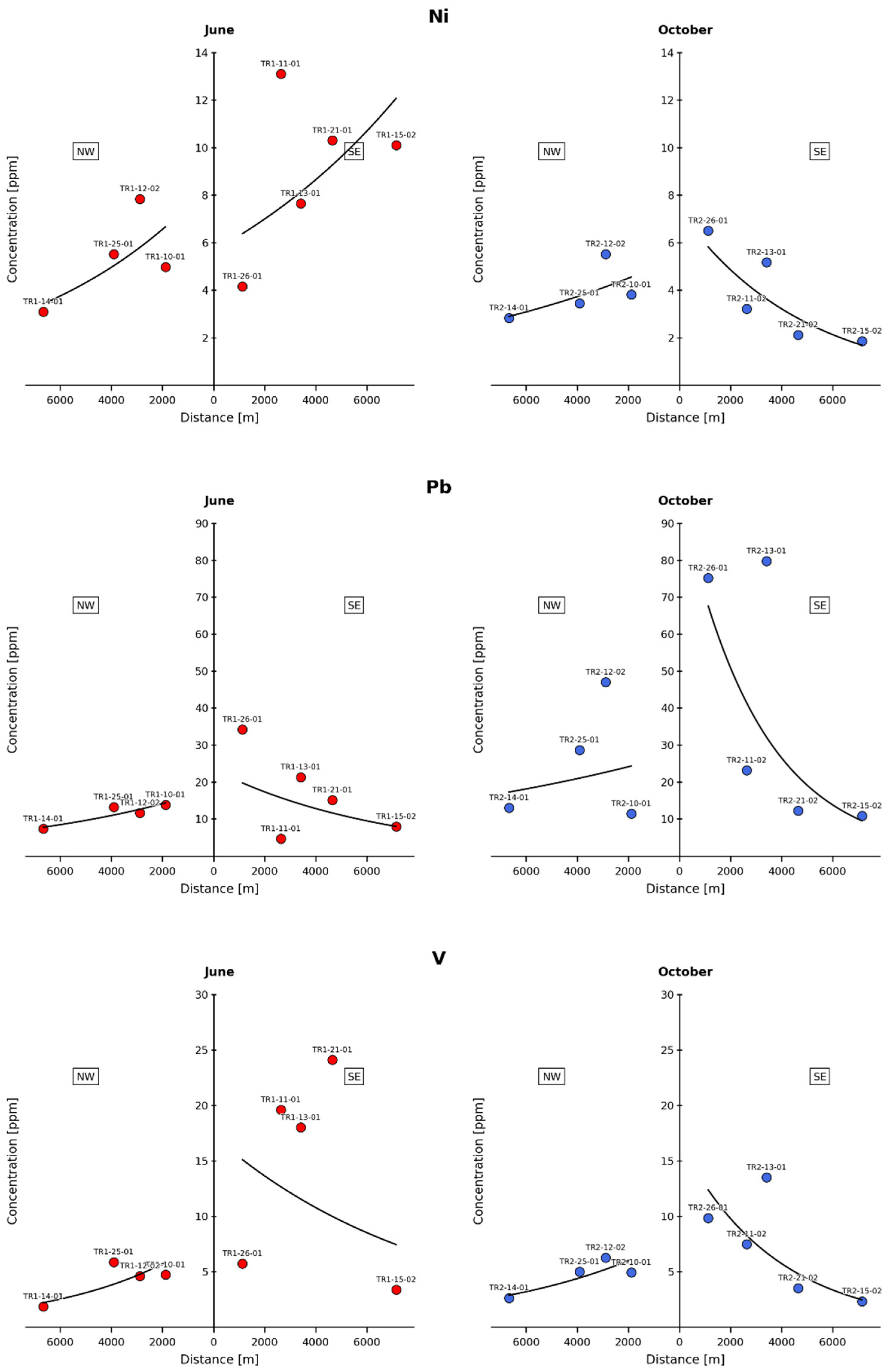
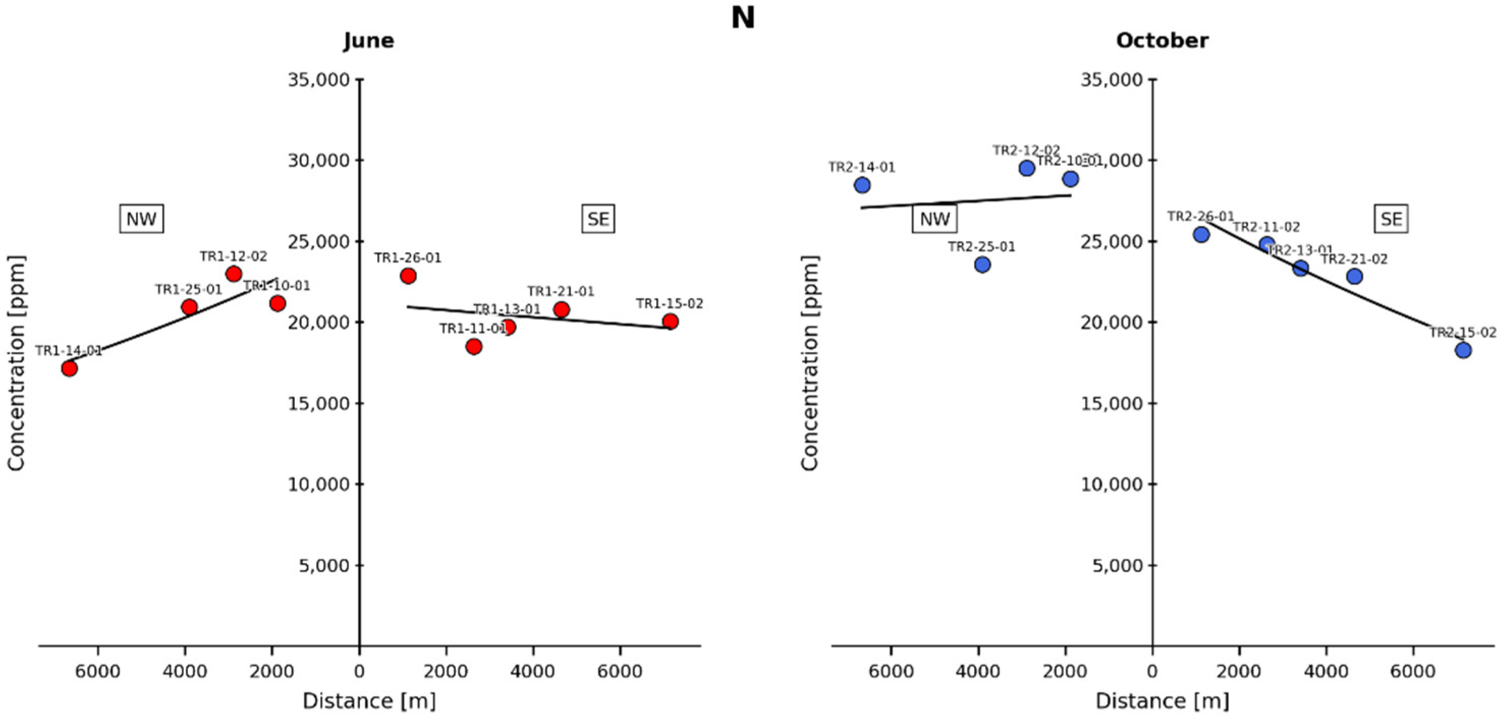
3.3. Spatial Distribution of Elements
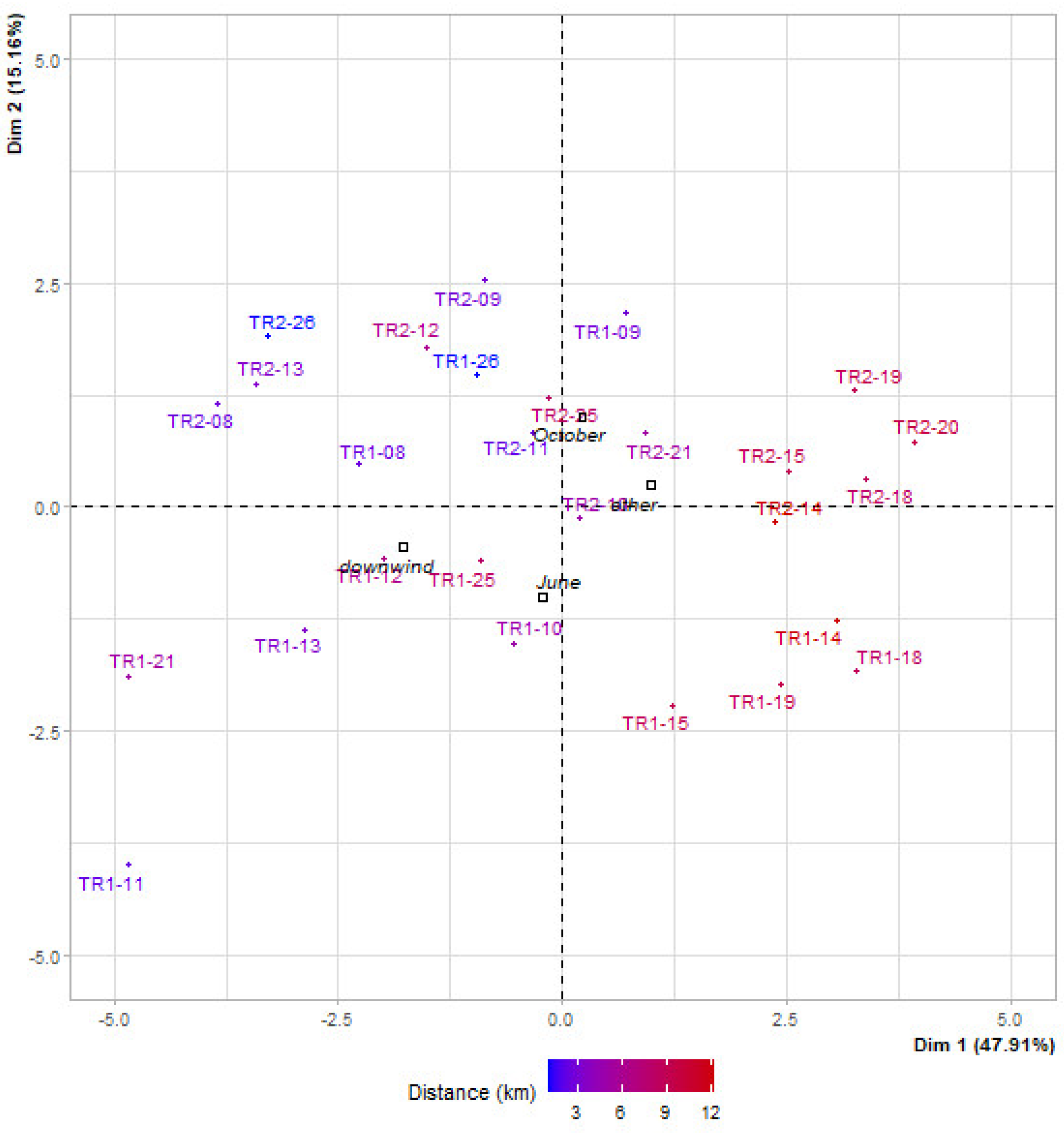
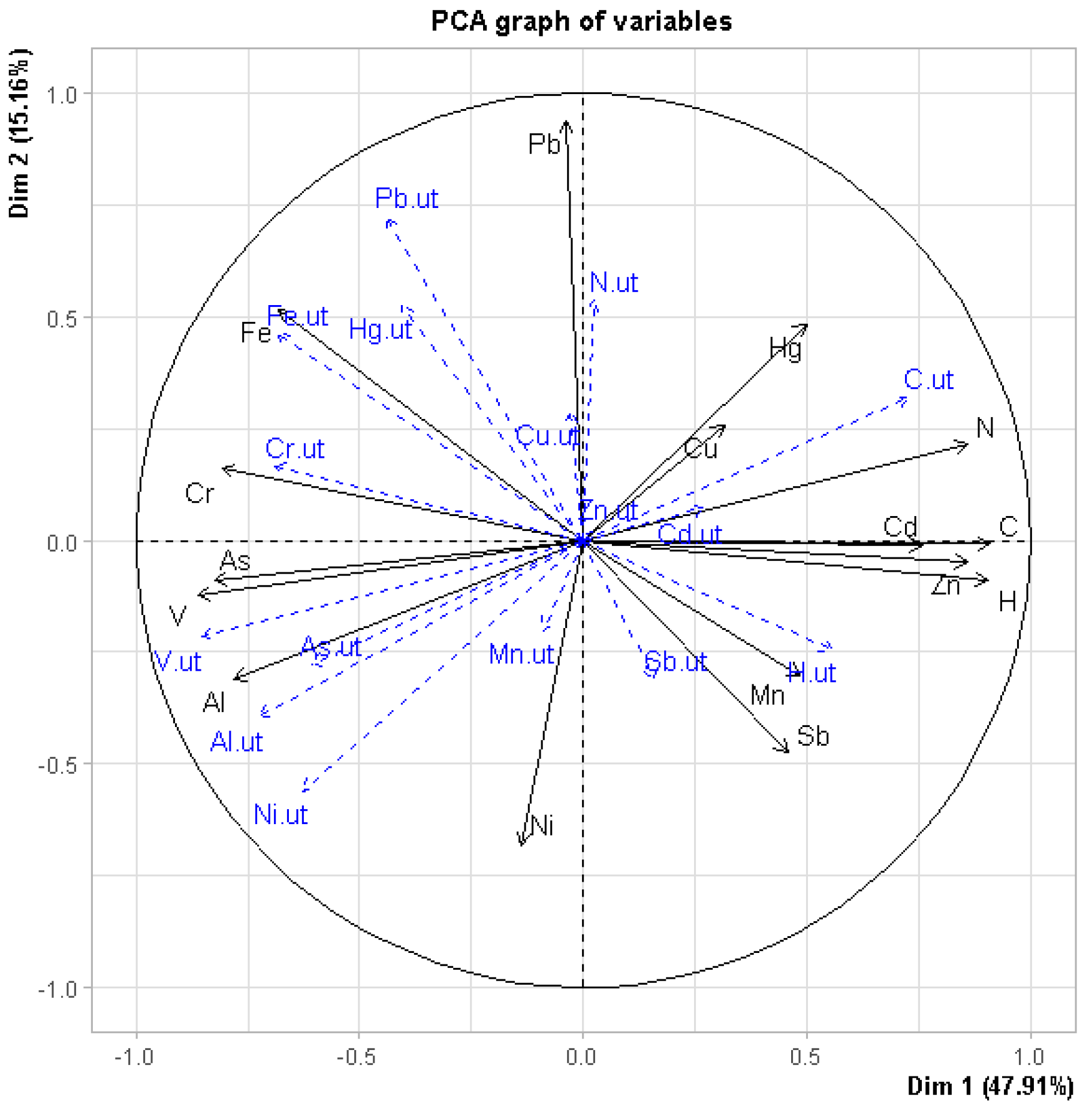
3.4. Principal Component Analysis (PCA)
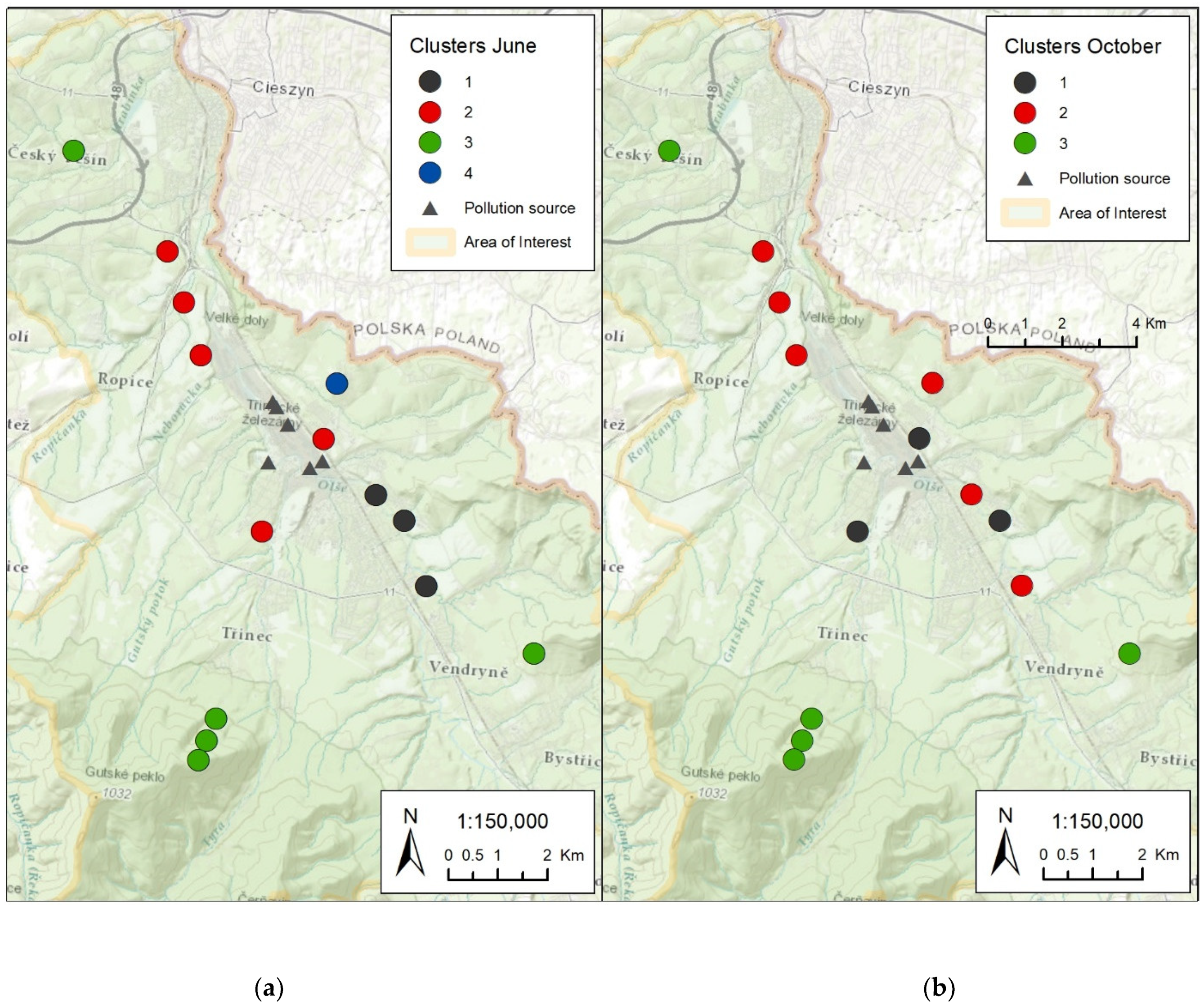
3.5. Hierarchical Clustering on Principal Components
4. Discussion
5. Conclusions
Supplementary Materials
Author Contributions
Funding
Institutional Review Board Statement
Informed Consent Statement
Data Availability Statement
Acknowledgments
Conflicts of Interest
Appendix A


References
- World Health Organization. Ambient Air Pollution: A Global Assessment of Exposure and Burden of Disease; World Health Organization: Geneva, Switzerland, 2016; ISBN 978-92-4-151135-3. [Google Scholar]
- Maynard, R.; Krzyzanowski, M.; Vilahur, N.; Héroux, M.-E. Evolution of WHO Air Quality Guidelines Past, Present and Future; Weltgesundheitsorganisation Regionalbüro für Europa: Copenhagen, Denmark, 2017; ISBN 978-92-890-5230-6. [Google Scholar]
- Czech Hydrometeorological Institute CHMI-Tabular Survey, Air Pollution and Atmospheric Deposition in Data, the Czech Republic. 2017. Available online: https://www.chmi.cz/files/portal/docs/uoco/isko/tab_roc/2017_enh/index_GB.html (accessed on 14 April 2020).
- European Environment Agency. Air Quality in Europe: 2019 Report; European Environment Agency: Copenhagen, Denmark, 2019; ISBN 978-92-9480-088-6. [Google Scholar]
- Hůnová, I. Ambient Air Quality in the Czech Republic: Past and Present. Atmosphere 2020, 11, 214. [Google Scholar] [CrossRef] [Green Version]
- Hůnová, I. Ambient Air Quality in the Czech Republic. Atmosphere 2021, 12, 770. [Google Scholar] [CrossRef]
- Ďurčanská, D. (Ed.) Riadenie Kvality Ovzdušia/Zarządzanie Jakością Powietrza, 1st ed.; EDIS–vydavateľské centrum, Žilinská univerzita v Žiline: Žilina, Slovakia, 2020; ISBN 978-80-554-1658-8. [Google Scholar]
- Ohara, T. Long-Range Transport and Deposition of Air Pollution. In Encyclopedia of Environmental Health; Elsevier: Amsterdam, The Netherlands, 2019; pp. 126–130. ISBN 978-0-444-63952-3. [Google Scholar]
- European Council. Directive 2008/50/EC of the European Parliament and of the Council of 21 May 2008 on Ambient Air Quality and Cleaner Air for Europe; European Council: Luxembourg, 2008; Volume L 152, pp. 1–44. [Google Scholar]
- European Council. Directive 2010/75/EU of the European Parliament and of the Council of 24 November 2010 on Industrial Emissions (Integrated Pollution Prevention and Control); European Council: Luxembourg, 2010; Volume L 334/17, p. 103. [Google Scholar]
- Commission of the European Union; Joint Research Centre; Institute for Prospective Technological Studies. Best Available Techniques (BAT) Reference Document for Iron and Steel Production: Industrial Emissions Directive 2010/75/EU: Integrated Pollution Prevention and Control; Publications Office: Luxembourg, 2013. [Google Scholar]
- Ghosh, A.; Chatterjee, A. Ironmaking and Steelmaking: Theory and Practice; Eastern Economy Edition; 3. Print; PHI Learning: New Delhi, India, 2010; ISBN 978-81-203-3289-8. [Google Scholar]
- Lin, B.; Xu, M. Regional Differences on CO2 Emission Efficiency in Metallurgical Industry of China. Energy Policy 2018, 120, 302–311. [Google Scholar] [CrossRef]
- Cholakov, G.S.; Nath, B. Pollution Control Technologies; Eolss Publishers Co. Ltd.: Oxford, UK, 2009; Volume 3, ISBN 978-1-84826-568-4. [Google Scholar]
- Tchounwou, P.B.; Yedjou, C.G.; Patlolla, A.K.; Sutton, D.J. Heavy Metal Toxicity and the Environment. In Molecular, Clinical and Environmental Toxicology; Springer: Basel, Switzerland, 2012; pp. 133–164. [Google Scholar]
- World Health Organization. Review of Evidence on Health Aspects of Air Pollution–REVIHAAP Project Technical Report; World Health Organization: Copenhagen, Denmark, 2013; p. 309. [Google Scholar]
- Fortoul, T.I.; Rodriguez-Lara, V.; Gonzalez-Villalva, A.; Rojas-Lemus, M.; Colin-Barenque, L.; Bizarro-Nevares, P.; García-Peláez, I.; Ustarroz-Cano, M.; López-Zepeda, S.; Cervantes-Yépez, S.; et al. Health Effects of Metals in Particulate Matter. In Current Air Quality Issues; Nejadkoorki, F., Ed.; InTech: London, UK, 2015; ISBN 978-953-51-2180-0. [Google Scholar]
- Seigneur, C. Air Pollution: Concepts, Theory, and Applications; Cambridge University Press: Cambridge, UK; New York, NY, USA, 2019; ISBN 978-1-108-48163-2. [Google Scholar]
- Elichegaray, C. (Ed.) La Pollution de l’air: Sources, Effets, Prévention; Universciences. Sciences de la vie; Dunod: Paris, France, 2008; ISBN 978-2-10-051564-6. [Google Scholar]
- Schaap, D.M.; Hendriks, C.; Jonkers, S.; Builtjes, D.P. Impacts of Heavy Metal Emission on Air Quality and Ecosystems across Germany. Sources Transp. Depos. Potential Hazards 2018, 2018, 92. [Google Scholar]
- Riffault, V.; Arndt, J.; Marris, H.; Mbengue, S.; Setyan, A.; Alleman, L.Y.; Deboudt, K.; Flament, P.; Augustin, P.; Delbarre, H.; et al. Fine and Ultrafine Particles in the Vicinity of Industrial Activities: A Review. Crit. Rev. Environ. Sci. Technol. 2015, 45, 2305–2356. [Google Scholar] [CrossRef]
- Fernández, A.J.; Ternero, M.; Barragán, F.J.; Jiménez, J.C. An Approach to Characterization of Sources of Urban Airborne Particles through Heavy Metal Speciation. Chemosph. Glob. Chang. Sci. 2000, 2, 123–136. [Google Scholar] [CrossRef]
- Ragosta, M.; Caggiano, R.; D’Emilio, M.; Sabia, S.; Trippetta, S.; Macchiato, M. PM10 and Heavy Metal Measurements in an Industrial Area of Southern Italy. Atmos. Res. 2006, 81, 304–319. [Google Scholar] [CrossRef]
- Saroop, S.; Tamchos, S. 4-Monitoring and impact assessment approaches for heavy metals. In Heavy Metals in the Environment; Kumar, V., Sharma, A., Cerdà, A., Eds.; Elsevier: Amsterdam, The Netherlands, 2021; pp. 57–86. ISBN 978-0-12-821656-9. [Google Scholar]
- Markert, B.A.; Breure, A.M.; Zechmeister, H.G. (Eds.) Bioindicators & Biomonitors: Principles, Concepts, and Applications; Trace metals and other contaminants in the environment; Elsevier: Amsterdam, The Netherlands; Boston, MA, USA, 2003; ISBN 978-0-08-044177-1. [Google Scholar]
- Frontasyeva, M.; Harmens, H. Monitoring of Atmospheric Deposition of Heavy Metals, Nitrogen and POPs in Europe Using Bryophytes: Monitoring Manual: Survey 2020. 2020. Available online: https://icpvegetation.ceh.ac.uk/sites/default/files/Moss%20protocol%20manual.pdf (accessed on 1 September 2021).
- Harmens, H.; Norris, D.; Mills, G. Convention on Long-range Transboundary Air Pollution. In Working Group on Effects Heavy Metals and Nitrogen in Mosses: Spatial Patterns in 2010/2011 and Long-Term Temporal Trends in Europe; Centre for Ecology & Hydrology: Bangor, Maine, 2013; ISBN 978-1-906698-38-6. [Google Scholar]
- Harmens, H.; Mills, G.; Hayes, F.; Norris, D.A.; Sharps, K. Twenty eight years of icp vegetation: An overview of its activities. Ann. Bot. 2015, 5, 31–43. [Google Scholar] [CrossRef]
- Schröder, W.; Nickel, S.; Schönrock, S.; Meyer, M.; Wosniok, W.; Harmens, H.; Frontasyeva, M.V.; Alber, R.; Aleksiayenak, J.; Barandovski, L.; et al. Spatially Valid Data of Atmospheric Deposition of Heavy Metals and Nitrogen Derived by Moss Surveys for Pollution Risk Assessments of Ecosystems. Environ. Sci. Pollut. Res. 2016, 23, 10457–10476. [Google Scholar] [CrossRef] [Green Version]
- Frontasyeva, M.; Harmens, H. Monitoring of Atmospheric Deposition of Heavy Metals, Nitrogen and POPs in Europe Using Bryophytes: Survey 2015: Monitoring Manual. 2015. Available online: https://icpvegetation.ceh.ac.uk/sites/default/files/ICP%20Vegetation%20moss%20monitoring%20manual%202020.pdf (accessed on 1 September 2021).
- Frontasyeva, M.V.; Steinnes, E. Epithermal Neutron Activation Analysis of Mosses Used to Monitor Heavy Metal Deposition around an Iron Smelter Complex. Analyst 1995, 120, 1437. [Google Scholar] [CrossRef]
- Frontasyeva, M.V.; Steinnes, E. Heavy Metal Atmospheric Deposition around an Iron Smelter Complex Studied by the Moss Biomonitoring Technique. In Air Pollution in the Ural Mountains: Environmental, Health and Policy Aspects; Linkov, I., Wilson, R., Eds.; Springer: Dordrecht, The Netherlands, 1998; pp. 383–389. ISBN 978-94-011-5208-2. [Google Scholar]
- Zechmeister, H.G.; Riss, A.; Hanus-Illnar, A. Biomonitoring of Atmospheric Heavy Metal Deposition by Mosses in the Vicinity of Industrial Sites. J. Atmos. Chem. 2004, 49, 461–477. [Google Scholar] [CrossRef]
- Suchara, I.; Sucharová, J. Mercury Distribution around the Spolana Chlor-Alkali Plant (Central Bohemia, Czech Republic) after a Catastrophic Flood, as Revealed by Bioindicators. Environ. Pollut. 2008, 151, 352–361. [Google Scholar] [CrossRef]
- Uyar, G.; Ören, M.; Yildirim, Y.; Öncel, S. Biomonitoring of Metal Deposition in the Vicinity of Eregli Steel Plant in Turkey. Environ. Forensics 2008, 9, 350–363. [Google Scholar] [CrossRef]
- Samecka-Cymerman, A.; Stankiewicz, A.; Kolon, K.; Kempers, A.J. Bioindication of Trace Metals in Brachythecium Rutabulum Around a Copper Smelter in Legnica (Southwest Poland): Use of a New Form of Data Presentation in the Form of a Self-Organizing Feature Map. Arch. Environ. Contam. Toxic. 2009, 56, 717–722. [Google Scholar] [CrossRef] [PubMed]
- González-Miqueo, L.; Elustondo, D.; Lasheras, E.; Santamaría, J.M. Use of Native Mosses as Biomonitors of Heavy Metals and Nitrogen Deposition in the Surroundings of Two Steel Works. Chemosphere 2010, 78, 965–971. [Google Scholar] [CrossRef] [PubMed]
- Bačeva, K.; Stafilov, T.; Šajn, R.; Tănăselia, C. Moss Biomonitoring of Air Pollution with Heavy Metals in the Vicinity of a Ferronickel Smelter Plant. J. Environ. Sci. Health Part A 2012, 47, 645–656. [Google Scholar] [CrossRef]
- Cowden, P.; Aherne, J. Assessment of Atmospheric Metal Deposition by Moss Biomonitoring in a Region under the Influence of a Long Standing Active Aluminium Smelter. Atmos. Environ. 2019, 201, 84–91. [Google Scholar] [CrossRef]
- Kapusta, P.; Stanek, M.; Szarek-Łukaszewska, G.; Godzik, B. Long-Term Moss Monitoring of Atmospheric Deposition near a Large Steelworks Reveals the Growing Importance of Local Non-Industrial Sources of Pollution. Chemosphere 2019, 230, 29–39. [Google Scholar] [CrossRef]
- European Committee for Standardization. CSN EN 16414 Ambient Air-Biomonitoring with Mosses-Accumulation of Atmospheric Contaminants in Mosses Collected in Situ: From the Collection to the Preparation of Samples; European Committee for Standardization: Brussels, Belgium, 2014. [Google Scholar]
- Pöykiö, R.; Tervaniemi, O.-M.; Torvela, H.; Perämäki, P. Heavy Metal Accumulation in Woodland Moss (Pleurozium Schreberi) in the Area Around a Chromium Opencast Mine at Kemi, and in the Area Around the Ferrochrome and Stainless Steel Works at Tornio, Northern Finland. Int. J. Environ. Anal. Chem. 2001, 81, 137–151. [Google Scholar] [CrossRef]
- Fernández, J.A.; Aboal, J.R.; Couto, J.A.; Carballeira, A. Moss Bioconcentration of Trace Elements around a FeSi Smelter: Modelling and Cellular Distribution. Atmos. Environ. 2004, 38, 4319–4329. [Google Scholar] [CrossRef]
- Varela, Z.; Aboal, J.R.; Carballeira, A.; Real, C.; Fernández, J.A. Use of a Moss Biomonitoring Method to Compile Emission Inventories for Small-Scale Industries. J. Hazard. Mater. 2014, 275, 72–78. [Google Scholar] [CrossRef]
- Motyka, O.; Pavlíková, I.; Bitta, J.; Frontasyeva, M.; Jančík, P. Moss Biomonitoring and Air Pollution Modelling on a Regional Scale: Delayed Reflection of Industrial Pollution in Moss in a Heavily Polluted Region? Environ. Sci. Pollut. Res. 2020, 27, 32569–32578. [Google Scholar] [CrossRef]
- Svozilík, V.; Svozilíková Krakovská, A.; Bitta, J.; Jančík, P. Comparison of the Air Pollution Mathematical Model of PM10 and Moss Biomonitoring Results in the Tritia Region. Atmosphere 2021, 12, 656. [Google Scholar] [CrossRef]
- Kottek, M.; Grieser, J.; Beck, C.; Rudolf, B.; Rubel, F. World Map of the Köppen-Geiger Climate Classification Updated. Meteorol. Z. 2006, 15, 259–263. [Google Scholar] [CrossRef]
- Český hydrometeorologický ústav. Univerzita Palackého v Olomouci Atlas Podnebí Česka (Climate Atlas of Czechia); Český hydrometeorologický ústav: Praha, Czech Republic; Univerzita Palackého v Olomouci: Olomouc, Czech Republic, 2007; Vydání 1, ISBN 978-80-86690-26-1. [Google Scholar]
- Třinecké železárny, A.S. Annual Report 2019; Třinec Iron and Steel Works: Třinec, Czech Republic, 2020. [Google Scholar]
- Czech Hydrometeorological Institute. CHMI-Tabular Survey, Air Pollution and Atmospheric Deposition in Data, the Czech Republic. 2019. Available online: https://www.chmi.cz/files/portal/docs/uoco/isko/tab_roc/2019_enh/index_GB.html (accessed on 14 April 2020).
- Czech Hydrometeorological Institute. CHMI-Tabular Survey, Air Pollution and Atmospheric Deposition in Data, the Czech Republic. 2018. Available online: http://portal.chmi.cz/files/portal/docs/uoco/isko/tab_roc/2018_enh/index_GB.html (accessed on 14 April 2020).
- Czech Hydrometeorological Institute Počasí: Denní Data dle Zákona 123/1998 Sb./Weather: Daily Data According to the Law No 123/1998 Co. Available online: https://www.chmi.cz/historicka-data/pocasi/denni-data/Denni-data-dle-z.-123-1998-Sb (accessed on 1 September 2021). (In Czech).
- Czech Hydrometeorological Institute. Informace o Kvalitě Ovzduší v ČR: Poskytování dat Podle Zákona č. 123/1998 Sb./Information on Air Quality in Czechia: Data Access According to the Law No 123/1998 Co. Available online: https://www.chmi.cz/files/portal/docs/uoco/historicka_data/OpenIsko_data/index.html. (accessed on 1 September 2021). (In Czech).
- Kłos, A.; Ziembik, Z.; Rajfur, M.; Dołhańczuk-Śródka, A.; Bochenek, Z.; Bjerke, J.W.; Tømmervik, H.; Zagajewski, B.; Ziółkowski, D.; Jerz, D.; et al. Using Moss and Lichens in Biomonitoring of Heavy-Metal Contamination of Forest Areas in Southern and North-Eastern Poland. Sci. Total Environ. 2018, 627, 438–449. [Google Scholar] [CrossRef]
- Schröder, W.; Pesch, R.; Englert, C.; Harmens, H.; Suchara, I.; Zechmeister, H.G.; Thöni, L.; Maňkovská, B.; Jeran, Z.; Grodzinska, K.; et al. Metal Accumulation in Mosses across National Boundaries: Uncovering and Ranking Causes of Spatial Variation. Environ. Pollut. 2008, 151, 377–388. [Google Scholar] [CrossRef] [PubMed] [Green Version]
- Fernández, J.A.; Boquete, M.T.; Carballeira, A.; Aboal, J.R. A Critical Review of Protocols for Moss Biomonitoring of Atmospheric Deposition: Sampling and Sample Preparation. Sci. Total Environ. 2015, 517, 132–150. [Google Scholar] [CrossRef] [PubMed]
- Meyer, M.; Schröder, W.; Nickel, S.; Leblond, S.; Lindroos, A.-J.; Mohr, K.; Poikolainen, J.; Santamaria, J.M.; Skudnik, M.; Thöni, L.; et al. Relevance of Canopy Drip for the Accumulation of Nitrogen in Moss Used as Biomonitors for Atmospheric Nitrogen Deposition in Europe. Sci. Total Environ. 2015, 538, 600–610. [Google Scholar] [CrossRef]
- Skudnik, M.; Jeran, Z.; Batič, F.; Simončič, P.; Kastelec, D. Potential Environmental Factors That Influence the Nitrogen Concentration and Δ15N Values in the Moss Hypnum Cupressiforme Collected inside and Outside Canopy Drip Lines. Environ. Pollut. 2015, 198, 78–85. [Google Scholar] [CrossRef]
- Frey, W.; Blockeel, T.L. (Eds.) The Liverworts, Mosses and Ferns of Europe; English Edition; Harley Books: Colchester, UK, 2006; ISBN 978-0-946589-70-8. [Google Scholar]
- Vučković, I.; Špirić, Z.; Stafilov, T.; Kušan, V. Moss Biomonitoring of Air Pollution with Chromium in Croatia. J. Environ. Sci. Health Part A 2013, 48, 829–834. [Google Scholar] [CrossRef]
- Špirić, Z.; Vučković, I.; Stafilov, T.; Kušan, V.; Bačeva, K. Biomonitoring of Air Pollution with Mercury in Croatia by Using Moss Species and CV-AAS. Env. Monit. Assess. 2014, 186, 4357–4366. [Google Scholar] [CrossRef]
- Kolon, K.; Ruczakowska, A.; Samecka-Cymerman, A.; Kempers, A.J. Brachythecium Rutabulum and Betula Pendula as Bioindicators of Heavy Metal Pollution around a Chlor-Alkali Plant in Poland. Ecol. Indic. 2015, 52, 404–410. [Google Scholar] [CrossRef]
- Drobnik, J.; Stebel, A. Brachythecium Rutabulum, A Neglected Medicinal Moss. Hum. Ecol. 2018, 46, 133–141. [Google Scholar] [CrossRef] [Green Version]
- Dumas, J. Procedes de I’analyse Organique. Ann. Chim. Phys. 1831, 47, 198–205. [Google Scholar]
- R Core Team. The R Project; The R Foundation. 2020. Available online: https://www.r-project.org (accessed on 1 September 2021).
- van den Boogaart, K.G.; Tolosana-Delgado, R.; Bren, M. Package ‘Compositions’ 2021. Available online: https://cran.r-project.org/web/packages/compositions/compositions.pdf (accessed on 9 June 2020).
- Templ, M.; Hron, K.; Filzmoser, P.; Facevicova, K.; Kynclova, P.; Walach, J.; Pintar, V.; Chen, J.; Miksova, D.; Meindl, B.; et al. Package ‘RobCompositions’ 2020. Available online: https://cran.r-project.org/web/packages/robCompositions/robCompositions.pdf (accessed on 9 June 2020).
- Templ, M.; Hron, K.; Filzmoser, P. robCompositions: An R-package for Robust Statistical Analysis of Compositional Data. In Compositional Data Analysis; Pawlowsky-Glahn, V., Buccianti, A., Eds.; John Wiley & Sons, Ltd.: Chichester, UK, 2011; pp. 341–355. ISBN 978-1-119-97646-2. [Google Scholar]
- Lê, S.; Josse, J.; Husson, F. FactoMineR: An R Package for Multivariate Analysis. J. Stat. Soft. 2008, 25. [Google Scholar] [CrossRef] [Green Version]
- Husson, F.; Josse, J.; Le, S.; Mazet, J. Package ‘FactoMineR’ 2020. Available online: http://www.jstatsoft.org/v25/i01/ (accessed on 16 July 2020).
- Wei, T.; Simko, V. Package ‘Corrplot’ 2021. Available online: https://cran.r-project.org/web/packages/corrplot/corrplot.pdf (accessed on 9 June 2020).
- Carslaw, D.; Ropkins, K. Package ‘Openair’ 2020. Available online: https://cran.r-project.org/web/packages/openair/openair.pdf (accessed on 17 July 2020).
- ESRI World Imagery-Overview. Available online: https://www.arcgis.com/home/item.html?id=10df2279f9684e4a9f6a7f08febac2a9 (accessed on 16 August 2021).
- ESRI World Topographic Map-Overview. Available online: https://www.arcgis.com/home/item.html?id=7dc6cea0b1764a1f9af2e679f642f0f5 (accessed on 16 August 2021).
- Dray, S.; Josse, J. Principal Component Analysis with Missing Values: A Comparative Survey of Methods. Plant Ecol. 2015, 216, 657–667. [Google Scholar] [CrossRef]
- Aitchison, J. The Statistical Analysis of Compositional Data; Blackburn Press: Caldwell, NJ, USA, 2003; ISBN 978-1-930665-78-1. [Google Scholar]
- Pawlowsky-Glahn, V.; Buccianti, A. (Eds.) Compositional Data Analysis: Theory and Applications; Wiley: Chichester, UK; West Sussex, UK, 2011; ISBN 978-0-470-71135-4. [Google Scholar]
- Hristozova, G.; Marinova, S.; Motyka, O.; Svozilík, V.; Zinicovscaia, I. Multivariate Assessment of Atmospheric Deposition Studies in Bulgaria Based on Moss Biomonitors: Trends between the 2005/2006 and 2015/2016 Surveys. Environ. Sci. Pollut. Res. 2020, 27, 39330–39342. [Google Scholar] [CrossRef]
- Mullineaux, S.T.; McKinley, J.M.; Marks, N.J.; Scantlebury, D.M.; Doherty, R. Heavy Metal (PTE) Ecotoxicology, Data Review: Traditional vs. a Compositional Approach. Sci. Total Environ. 2021, 769, 145246. [Google Scholar] [CrossRef] [PubMed]
- Harmens, H.; Ilyin, I.; Mills, G.; Aboal, J.R.; Alber, R.; Blum, O.; Coşkun, M.; de Temmerman, L.; Fernández, J.Á.; Figueira, R.; et al. Country-Specific Correlations across Europe between Modelled Atmospheric Cadmium and Lead Deposition and Concentrations in Mosses. Environ. Pollut. 2012, 166, 1–9. [Google Scholar] [CrossRef] [PubMed] [Green Version]
- Schröder, W.; Pesch, R.; Hertel, A.; Schonrock, S.; Harmens, H.; Mills, G.; Ilyin, I. Correlation between Atmospheric Deposition of Cd, Hg and Pb and Their Concentrations in Mosses Specified for Ecological Land Classes Covering Europe. Atmos. Pollut. Res. 2013, 4, 267–274. [Google Scholar] [CrossRef] [Green Version]
- Schröder, W.; Pesch, R.; Schönrock, S.; Harmens, H.; Mills, G.; Fagerli, H. Mapping Correlations between Nitrogen Concentrations in Atmospheric Deposition and Mosses for Natural Landscapes in Europe. Ecol. Indic. 2014, 36, 563–571. [Google Scholar] [CrossRef] [Green Version]
- Nickel, S.; Schröder, W. Integrative Evaluation of Data Derived from Biomonitoring and Models Indicating Atmospheric Deposition of Heavy Metals. Environ. Sci. Pollut. Res. 2017, 24, 11919–11939. [Google Scholar] [CrossRef]
- Bubník, J.; Keder, J.; Macoun, J.; Maňák, J. SYMOS ’97: Systém modelování stacionárních zdrojů: Metodická příručka; Český hydrometeorologický ústav/Czech Hydrometeorological Institute: Prague, Czech Republic, 2014. (In Czech) [Google Scholar]
- Keder, J.; Bubník, J.; Srněnský, R. Report of the project implementation in 2002: Design of Model Tools for Objective Assessment of the State and Development of Air Pollution in Accordance with the New Air Law and EU Directives (Zpráva za řešení dílčího projektu DP2 v roce 2002: Návrh modelových nástrojů pro objektivní hodnocení stavu a vývoje znečištění ovzduší v souladu s novým zákonem o ovzduší a směrnicemi EU); Czech Hydrometeorologic Institute: Prague, Czech Republic, 2002; p. 20. (In Czech) [Google Scholar]
- Seibert, R.; Nikolova, I.; Volná, V.; Krejčí, B.; Hladký, D. Air Pollution Sources’ Contribution to PM2.5 Concentration in the North-eastern Part of the Czech Republic. Atmosphere 2020, 11, 522. [Google Scholar] [CrossRef]
- Hoek, G.; Beelen, R.; de Hoogh, K.; Vienneau, D.; Gulliver, J.; Fischer, P.; Briggs, D. A Review of Land-Use Regression Models to Assess Spatial Variation of Outdoor Air Pollution. Atmos. Environ. 2008, 42, 7561–7578. [Google Scholar] [CrossRef]
- Merbitz, H.; Fritz, S.; Schneider, C. Mobile Measurements and Regression Modeling of the Spatial Particulate Matter Variability in an Urban Area. Sci. Total Environ. 2012, 438, 389–403. [Google Scholar] [CrossRef] [PubMed]
- Filzmoser, P.; Hron, K.; Reimann, C. Univariate Statistical Analysis of Environmental (Compositional) Data: Problems and Possibilities. Sci. Total Environ. 2009, 407, 6100–6108. [Google Scholar] [CrossRef] [PubMed]
- Suchara, I.; Sucharová, J.; Holá, M. A Quarter Century of Biomonitoring Atmospheric Pollution in the Czech Republic. Environ. Sci. Pollut. Res. 2017, 24, 11949–11963. [Google Scholar] [CrossRef]
- Aboal, J.R.; Boquete, M.T.; Carballeira, A.; Casanova, A.; Debén, S.; Fernández, J.A. Quantification of the Overall Measurement Uncertainty Associated with the Passive Moss Biomonitoring Technique: Sample Collection and Processing. Environ. Pollut. 2017, 224, 235–242. [Google Scholar] [CrossRef]
- Schröder, W.; Nickel, S. Moss Species-Specific Accumulation of Atmospheric Deposition? Environ. Sci. Eur. 2019, 31, 78. [Google Scholar] [CrossRef] [Green Version]
- Sucharová, J.; Suchara, I. Bio-Monitoring the Atmospheric Deposition of Elements and Their Compounds Using Moss Analysis in the Czech Republic. Results of the International Bio-Monitoring Programme UNECE ICP-Vegetation 2000. Part I: Elements Required for the Bio-Monitoring Programme. Acta Pruhoniciana 2004, 77, 1–135. [Google Scholar]
- Sucharová, J.; Suchara, I.; Holá, M. Výzkumný ústav Silva Taroucy pro krajinu a okrasné zahradnictví; Oddělení Biomonitoringu Contents of 37 Elements in Moss and Their Temporal and Spatial Trends in the Czech Republic during the Last 15 Years: Fourth Czech bio-monitoring survey pursued in the framework of the international programme UNECE ICP-Vegetation 2005/2006 = Obsah 37 prvků v mechu a časové a prostorové změny jeho hodnot v České republice během posledních 15 let: Čtvrtý český biomonitorovací průzkum prováděný v rámci mezinárodního programu OSN EHK ICP-Vegetace 2005/2006; Výzkumný ústav Silva Taroucy pro krajinu a okrasné zahradnictví: Průhonice, Czech Republic; Nová tiskárna Pelhřimov: Pelhřimov, Czech Republic, 2008; ISBN 978-80-85116-62-5. [Google Scholar]
- Jenner, F.E.; StC O’Neill, H. Lithophile Elements. In Encyclopedia of Geochemistry; White, W.M., Ed.; Encyclopedia of Earth Sciences Series; Springer International Publishing: Cham, Switzerland, 2018; pp. 827–828. ISBN 978-3-319-39311-7. [Google Scholar]
- Barnes, S.-J. Chalcophile Elements. In Encyclopedia of Geochemistry; White, W.M., Ed.; Encyclopedia of Earth Sciences Series; Springer International Publishing: Cham, Switzerland, 2018; pp. 229–233. ISBN 978-3-319-39311-7. [Google Scholar]
- Zechmeister, H.G.; Richter, A.; Smidt, S.; Hohenwallner, D.; Roder, I.; Maringer, S.; Wanek, W. Total Nitrogen Content and δ 15 N Signatures in Moss Tissue: Indicative Value for Nitrogen Deposition Patterns and Source Allocation on a Nationwide Scale. Environ. Sci. Technol. 2008, 42, 8661–8667. [Google Scholar] [CrossRef]
- Boquete, M.T.; Fernández, J.A.; Aboal, J.R.; Carballeira, A. Are Terrestrial Mosses Good Biomonitors of Atmospheric Deposition of Mn? Atmos. Environ. 2011, 45, 2704–2710. [Google Scholar] [CrossRef]
- Sylvestre, A.; Mizzi, A.; Mathiot, S.; Masson, F.; Jaffrezo, J.L.; Dron, J.; Mesbah, B.; Wortham, H.; Marchand, N. Comprehensive Chemical Characterization of Industrial PM2.5 from Steel Industry Activities. Atmos. Environ. 2017, 152, 180–190. [Google Scholar] [CrossRef]
- Pernigotti, D.; Belis, C.A.; Spanò, L. SPECIEUROPE: The European Data Base for PM Source Profiles. Atmos. Pollut. Res. 2016, 7, 307–314. [Google Scholar] [CrossRef]
- Bray, C.D.; Strum, M.; Simon, H.; Riddick, L.; Kosusko, M.; Menetrez, M.; Hays, M.D.; Rao, V. An Assessment of Important SPECIATE Profiles in the EPA Emissions Modeling Platform and Current Data Gaps. Atmos. Environ. 2019, 207, 93–104. [Google Scholar] [CrossRef]
- Robl, T.L.; Oberlink, A.; Jones, R. (Eds.) Coal Combustion Products (CCPs): Characteristics, Utilization and Beneficiation; Woodhead series in energy; Woodhead Publishing, an imprint of Elsevier: Cambridge, UK, 2017; ISBN 978-0-08-100945-1. [Google Scholar]


| Variable | Min | Mean | Median | Max | MAD | Skewness | Kurtosis |
|---|---|---|---|---|---|---|---|
| June Al | 0.05 | 0.36 | 0.18 | 1.20 | 0.097 | 1.5 | 0.4 |
| October Al | 0.07 | 0.21 | 0.17 | 0.70 | 0.069 | 2.3 | 6.2 |
| June V | 1.4 | 7.7 | 4.7 | 24.1 | 2.6 | 1.3 | 0.3 |
| October V | 2.1 | 6.2 | 5.0 | 19.3 | 2.5 | 1.7 | 2.7 |
| June Cr | 2.9 | 15.6 | 14.3 | 39.4 | 6.2 | 1.0 | 0.9 |
| October Cr | 4.1 | 18.9 | 14.8 | 87.4 | 8.9 | 2.8 | 8.9 |
| June Mn | 122.0 | 334.7 | 327.5 | 718.0 | 108.0 | 1.1 | 1.7 |
| October Mn | 93.3 | 320.6 | 259.0 | 843.0 | 58.0 | 1.9 | 4.9 |
| June Fe | 0.12 | 0.70 | 0.70 | 1.20 | 0.423 | −0.1 | −1.8 |
| October Fe | 0.2 | 1.0 | 0.6 | 2.5 | 0.393 | 0.8 | −0.8 |
| June Ni | 2.4 | 6.0 | 4.8 | 13.1 | 1.9 | 1.0 | −0.03 |
| October Ni | 1.9 | 3.5 | 3.3 | 6.5 | 0.9 | 0.9 | −0.01 |
| June Cu | 5.1 | 15.3 | 9.1 | 99.7 | 1.7 | 3.7 | 13.7 |
| October Cu | 4.7 | 7.9 | 7.1 | 16.9 | 1.8 | 1.9 | 5.1 |
| June Zn | 73.4 | 116.7 | 112.5 | 159.0 | 17.5 | 0.1 | −0.5 |
| October Zn | 69.9 | 108.2 | 102.8 | 156.0 | 26.2 | 0.4 | −1.2 |
| June As | <1.0 | 2.7 | 0.5 | 14.6 | 0.5 | 1.8 | 2.4 |
| October As | <1.0 | 1.0 | 5.1 | 1.9 | 2.4 | ||
| June Cd | 1.0 | 1.5 | 1.4 | 3.0 | 0.33 | 1.7 | 3.0 |
| October Cd | 0.6 | 1.7 | 1.5 | 4.5 | 0.35 | 1.9 | 4.2 |
| June Sb | <1.0 | 1.0 | 1.2 | 2.7 | 0.97 | 0.3 | −1.1 |
| June Hg | 0.041 | 0.075 | 0.074 | 0.108 | 0.016 | 0.01 | −1.2 |
| October Hg | 0.067 | 0.102 | 0.087 | 0.168 | 0.014 | 1.0 | −0.2 |
| June Pb | 4.62 | 19.11 | 12.4 | 70.1 | 4.75 | 2.1 | 4.4 |
| October Pb | 10.8 | 33.2 | 24.85 | 79.8 | 13.05 | 0.9 | −0.5 |
| June N | 1.6 | 2.1 | 2.1 | 2.7 | 0.159 | 0.4 | 1.3 |
| October N | 1.8 | 2.5 | 2.5 | 3.0 | 0.357 | −0.3 | v1.0 |
| Variable | Al | V | Cr | Mn | Fe | Ni | Cu | Zn | As | Cd | Sb | Hg | Pb | N |
|---|---|---|---|---|---|---|---|---|---|---|---|---|---|---|
| Třinec June | 1770 | 4.70 | 14.3 | 328 | 6960 | 4.8 | 9.1 | 112.5 | 0.50 | 1.4 | 1.2 | 0.074 | 12.4 | 20,872 |
| Třinec Oct. | 1730 | 5.00 | 14.8 | 259 | 6330 | 3.3 | 7.1 | 102.8 | 1.5 | 0.087 | 24.9 | 25,110 | ||
| Czechia [90] | 440 | 1.18 | 1.0 | 449 | 349 | 1.2 | 5.9 | 33.9 | 0.26 | 0.18 | 0.1 | 0.041 | 2.9 | 11,822 |
| Czechia In. [27] | 2.18 | 1.8 | 589 | 1.6 | 6.2 | 37.7 | 0.42 | 0.20 | 0.055 | 3.9 | 15,667 | |||
| Zumarraga [37] | 7.90 | 26.1 | 8.0 | 33.1 | 304.0 | 1.00 | 0.82 | 0.13 | 86.0 | |||||
| Azkoitia [37] | 4.99 | 13.7 | 14.9 | 17.7 | 250.0 | 1.25 | 0.41 | 0.07 | 40.7 | |||||
| Eregli 1 [35] | 5.1 | 3361 | 5.0 | 3.8 | 0.90 | 24.4 |
Publisher’s Note: MDPI stays neutral with regard to jurisdictional claims in published maps and institutional affiliations. |
© 2021 by the authors. Licensee MDPI, Basel, Switzerland. This article is an open access article distributed under the terms and conditions of the Creative Commons Attribution (CC BY) license (https://creativecommons.org/licenses/by/4.0/).
Share and Cite
Pavlíková, I.; Motyka, O.; Plášek, V.; Bitta, J. Monitoring of Heavy Metals and Nitrogen Concentrations in Mosses in the Vicinity of an Integrated Iron and Steel Plant: Case Study in Czechia. Appl. Sci. 2021, 11, 8262. https://0-doi-org.brum.beds.ac.uk/10.3390/app11178262
Pavlíková I, Motyka O, Plášek V, Bitta J. Monitoring of Heavy Metals and Nitrogen Concentrations in Mosses in the Vicinity of an Integrated Iron and Steel Plant: Case Study in Czechia. Applied Sciences. 2021; 11(17):8262. https://0-doi-org.brum.beds.ac.uk/10.3390/app11178262
Chicago/Turabian StylePavlíková, Irena, Oldřich Motyka, Vítězslav Plášek, and Jan Bitta. 2021. "Monitoring of Heavy Metals and Nitrogen Concentrations in Mosses in the Vicinity of an Integrated Iron and Steel Plant: Case Study in Czechia" Applied Sciences 11, no. 17: 8262. https://0-doi-org.brum.beds.ac.uk/10.3390/app11178262