
Evaluation of Seasonal and Spatial Variations in Water Quality and Identification of Potential Sources of Pollution Using Multivariate Statistical Techniques for Lake Hawassa Watershed, Ethiopia


Abstract
:1. Introduction
2. Materials and Methods
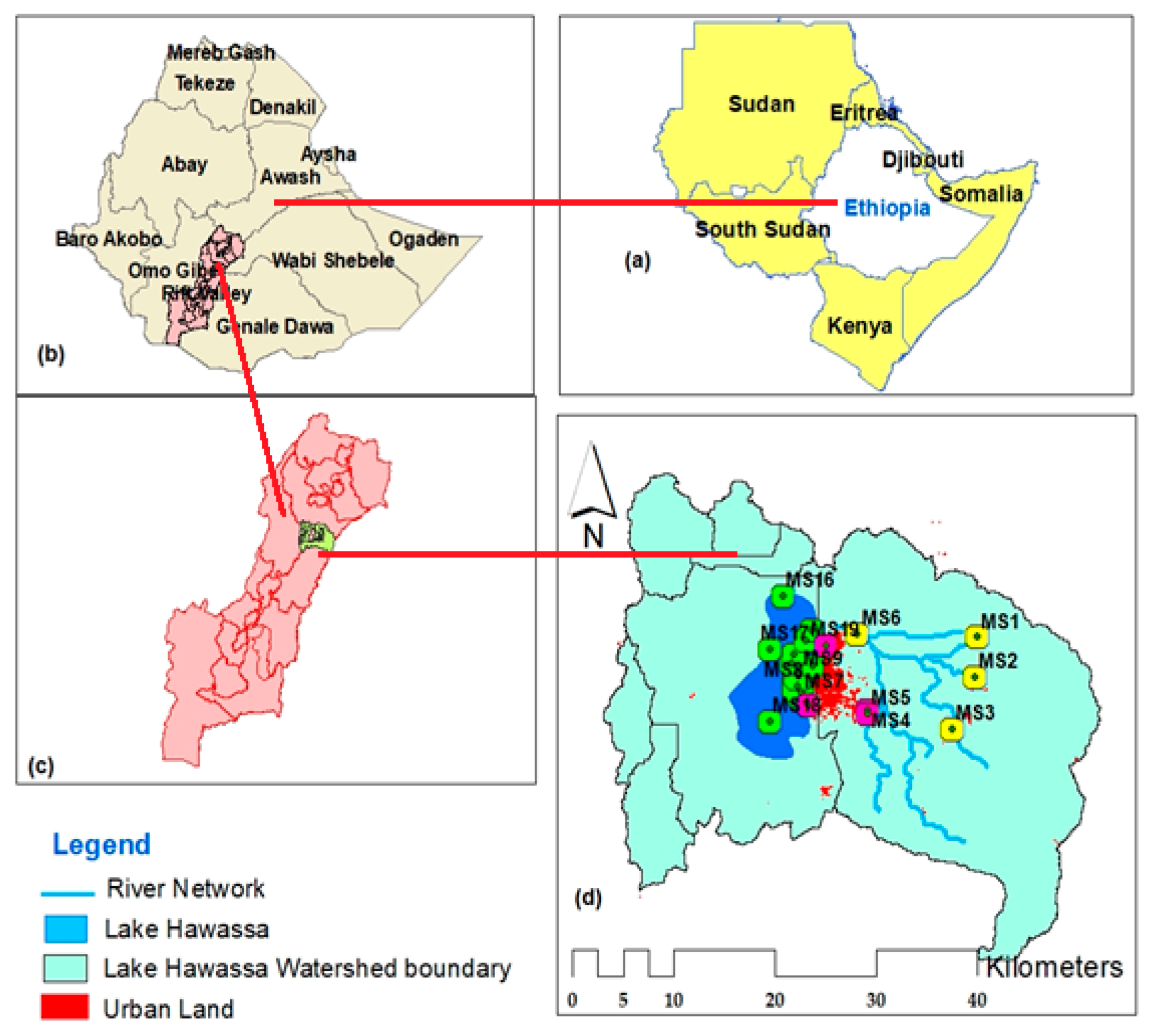
2.1. Study Area
2.2. Sampling and Monitoring Parameters
Un-Ionized Ammonia Determination from Total Ammonium Nitrogen (TAN)
3. Multivariate Statistical Techniques and Data Treatment
3.1. Multivariate Statistical Techniques
3.2. Data Treatment and Multivariate Statistical Methods
3.2.1. Principal Component (PCs)/Factor Analysis (FA)
3.2.2. Discriminant Analysis
3.2.3. Pollution Index (PI)
3.3. Cluster Analysis
4. Results and Discussion
4.1. Correlation Matrix Evaluation and Seasonal Variation
4.2. Pollution Index (PI)
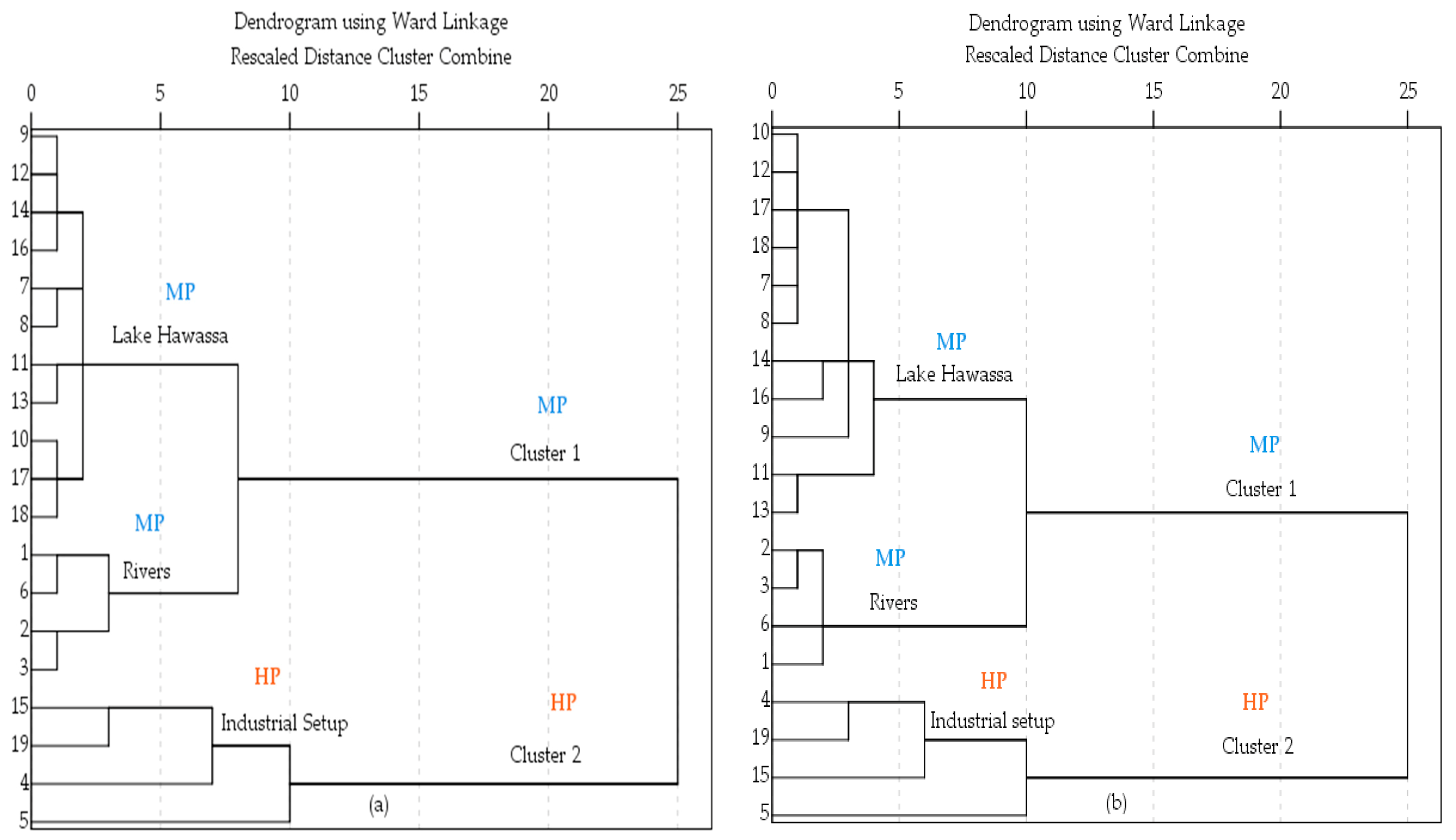
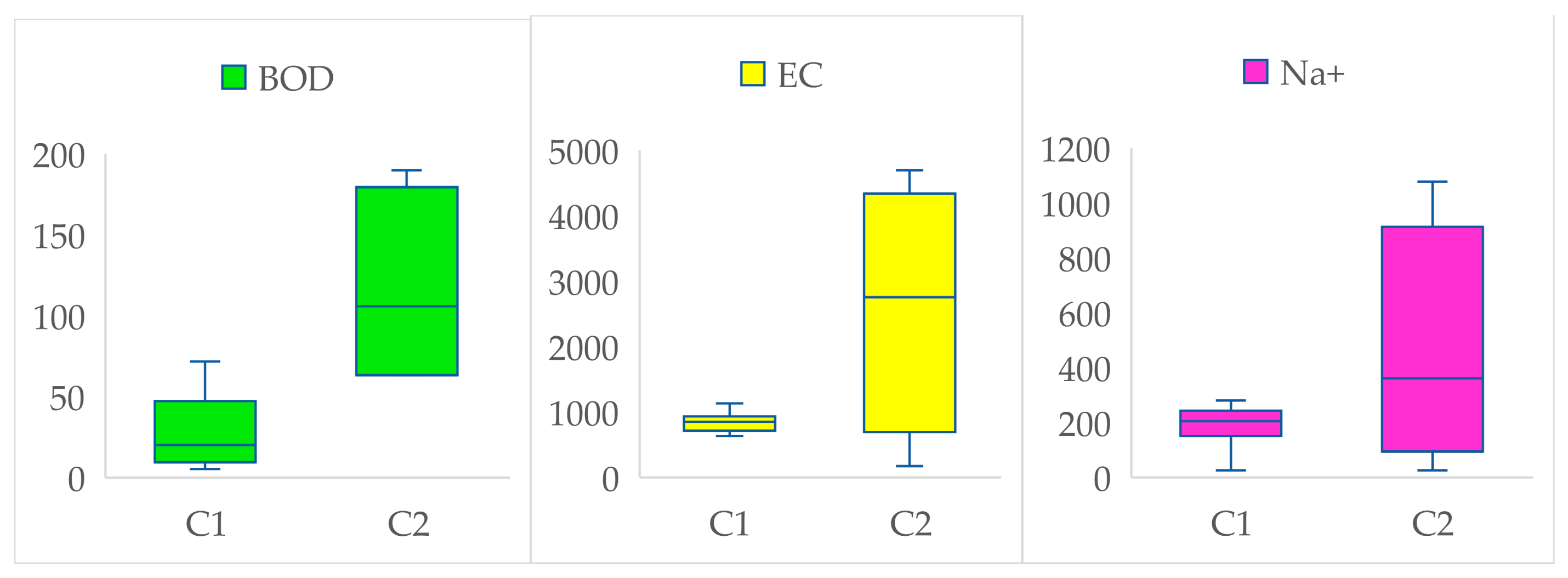
4.3. Cluster Analysis
Spatial and Temporal Similarities
4.4. Discriminant Analysis
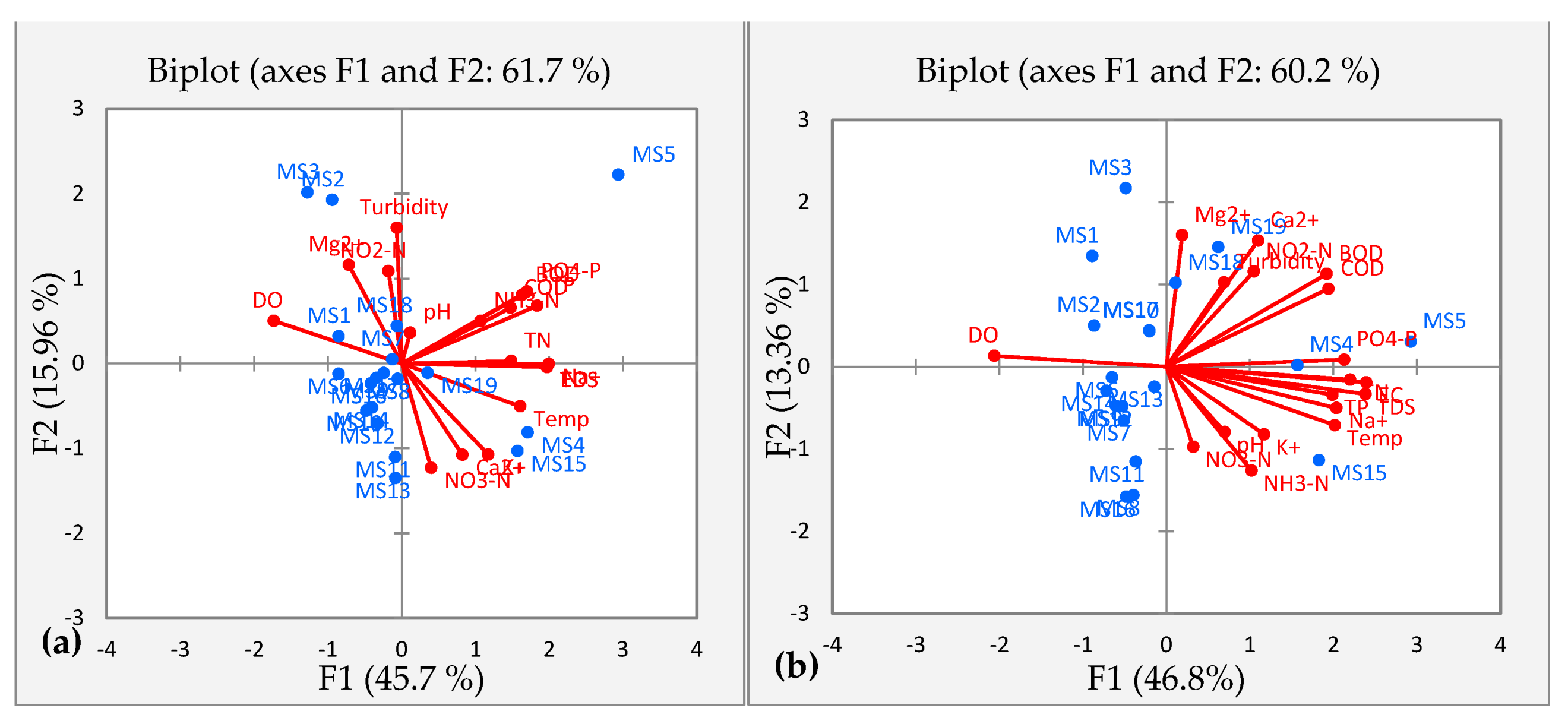
4.5. Pollution Source Identification of Monitored Variables
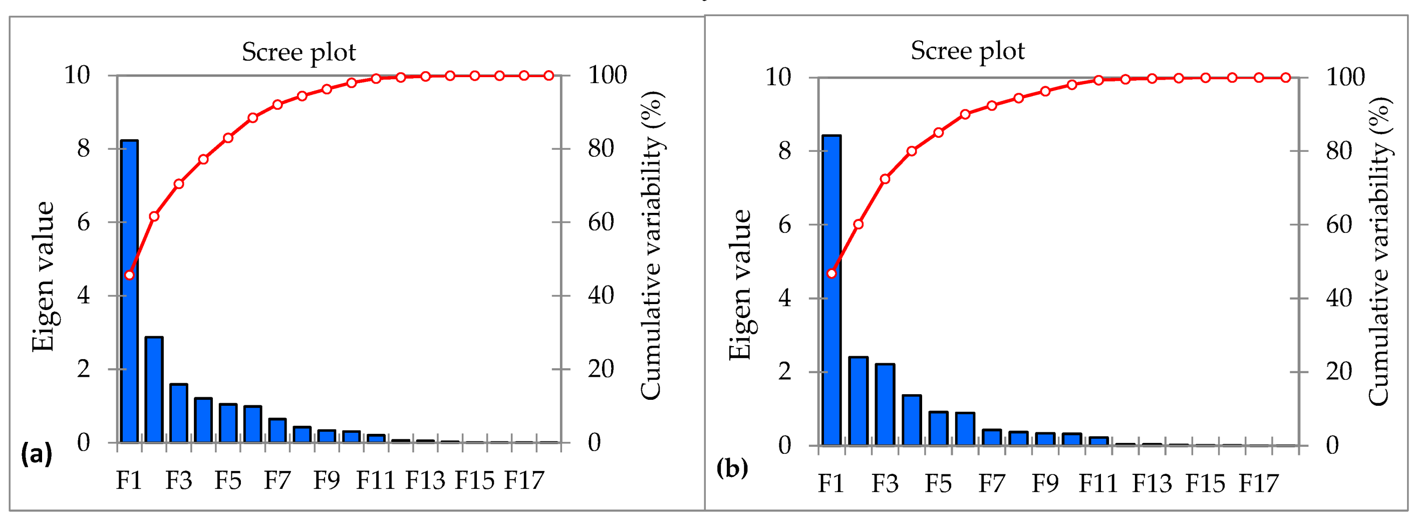
Principal Component Analysis
4.6. Total Nitrogen to Total Phosphorus (TN:TP) Ratio
5. Conclusions
Author Contributions
Funding
Institutional Review Board Statement
Informed Consent Statement
Data Availability Statement
Acknowledgments
Conflicts of Interest
References
- Cherif, E.K.; Salmoun, F.; Mesas-Carrascosa, F.J. Determination of Bathing Water Quality Using Thermal Images Landsat 8 on the West Coast of Tangier: Preliminary Results. Remote Sens. 2019, 11, 972. [Google Scholar] [CrossRef] [Green Version]
- Fan, X.; Cui, B.; Zhao, H.; Zhang, Z.; Zhang, H. Assessment of river water quality in Pearl River Delta using multivariate statistical techniques. Procedia Environ. Sci. 2010, 2, 1220–1234. [Google Scholar] [CrossRef] [Green Version]
- Noori, R.; Sabahi, M.; Karbassi, A.; Baghvand, A.; Zadeh, H.T. Multivariate statistical analysis of surface water quality based on correlations and variations in the data set. Desalination 2010, 260, 129–136. [Google Scholar] [CrossRef]
- Wang, Q.; Li, S.; Jia, P.; Qi, C.; Ding, F. A Review of Surface Water Quality Models. Sci. World J. 2013, 2013, 1–7. [Google Scholar] [CrossRef] [Green Version]
- Simeonov, V.; Stratis, J.; Samara, C.; Zachariadis, G.; Voutsa, D.; Anthemidis, A.; Sofoniou, M.; Kouimtzis, T. Assessment of the surface water quality in Northern Greece. Water Res. 2003, 37, 4119–4124. [Google Scholar] [CrossRef]
- Massoud, M.A.; El-Fadel, M.; Scrimshaw, M.D.; Lester, J.N. Factors influencing development of management strategies for the Abou Ali River in Lebanon. I: Spatial variation and land use. Sci. Total Environ. 2006, 362, 15–30. [Google Scholar] [CrossRef]
- Wang, X.-L.; Lu, Y.-L.; Han, J.-Y.; He, G.-Z.; Wang, T.-Y. Identification of anthropogenic influences on water quality of rivers in Taihu watershed. J. Environ. Sci. 2007, 19, 475–481. [Google Scholar] [CrossRef]
- Abebe, Y.D.; Geheb, K. Wetlands of Ethiopia. In Proceedings of a Seminar on the Resources and Status of Ethiopia’s Wetlands; IUCN, The World Conservation Union: Gland, Switzerland, 2003. [Google Scholar]
- Cherif, E.K.; Salmoun, F.; El Yemlahi, A.; Magalhaes, J.M. Monitoring Tangier (Morocco) coastal waters for As, Fe and P concentrations using ESA Sentinels-2 and 3 data: An exploratory study. Reg. Stud. Mar. Sci. 2019, 32, 100882. [Google Scholar] [CrossRef]
- Amare, T.A.; Yimer, G.T.; Workagegn, K.B. Assessment of Metal concentration in water, sediment and macrophyte plant collected from Lake Hawassa, Ethiopia. Environ. Anal. Toxicol. 2014, 05, 1–7. [Google Scholar] [CrossRef] [Green Version]
- Teshome, F.B. Seasonal water quality index and suitability of the water body to designated uses at the eastern catchment of Lake Hawassa. Environ. Sci. Pollut. Res. 2019, 27, 279–290. [Google Scholar] [CrossRef]
- Zigde, H.; Tsegaye, M.E. Evaluation of the current water quality of Lake Hawassa, Ethiopia. Int. J. Water Resour. Environ. Eng. 2019, 11, 120–128. [Google Scholar]
- Amare, D. Assessment of Non-Point Source Pollution in Lake Awassa Watershed Using the Annualized Agricultural Non-Point Source (AnnAGNPS) Model; Addis Ababa University: Addis Ababa, Ethiopia, 2008. [Google Scholar]
- Drevnick, P.E.; Engstrom, D.; Driscoll, C.T.; Swain, E.; Balogh, S.J.; Kamman, N.C.; Long, D.T.; Muir, D.; Parsons, M.J.; Rolfhus, K.R.; et al. Spatial and temporal patterns of mercury accumulation in lacustrine sediments across the Laurentian Great Lakes region. Environ. Pollut. 2012, 161, 252–260. [Google Scholar] [CrossRef] [PubMed] [Green Version]
- Kebede, W.; Tefera, M.; Habitamu, T.; Alemayehu, T. Impact of Land Cover Change on Water Quality and Stream Flow in Lake Hawassa Watershed of Ethiopia. Agric. Sci. 2014, 5, 647–659. [Google Scholar] [CrossRef] [Green Version]
- Lencha, S.M.; Tränckner, J.; Dananto, M. Assessing the Water Quality of Lake Hawassa Ethiopia—Trophic State and Suitability for Anthropogenic Uses—Applying Common Water Quality Indices. Int. J. Environ. Res. Public Health 2021, 18, 8904. [Google Scholar] [CrossRef]
- Nigussie, K.; Chandravanshi, B.S.; Wondimu, T. Correlation among trace metals in Tilapia (Oreochromis niloticus), sediment and water samples of lakes Awassa and Ziway, Ethiopia. Int. J. Biol. Chem. Sci. 2011, 4. [Google Scholar] [CrossRef] [Green Version]
- Wondrade, N.; Dick, Ø.B.; Tveite, H. GIS based mapping of land cover changes utilizing multi-temporal remotely sensed image data in Lake Hawassa Watershed, Ethiopia. Environ. Monit. Assess. 2014, 186, 1765–1780. [Google Scholar] [CrossRef]
- Abiye, T.A. Environmental resources and recent impacts in the Awassa collapsed caldera, Main Ethiopian Rift. Quat. Int. 2008, 189, 152–162. [Google Scholar] [CrossRef]
- APHA Standard Methods for the Examination of Water and Wastewater, 23rd ed.; Baird, R.B.; Eaton, A.D.; Rice, E.W.; Brigewater, L.L. (Eds.) American Public Health Association (APHA): Washington, DC, USA; American Water Works Association (AWWA): Washington, DC, USA; Water Environment Federati, Water Environment Federation: Washington, DC, USA, 2017; ISBN 9780123821652. [Google Scholar]
- Emerson, K.; Russo, R.C.; Lund, R.E.; Thurston, R.V. Aqueous Ammonia Equilibrium Calculations: Effect of pH and Temperature. J. Fish. Res. Board Can. 1975, 32, 2379–2383. [Google Scholar] [CrossRef]
- Angello, Z.A.; Tränckner, J.; Behailu, B.M. Spatio-Temporal Evaluation and Quantification of Pollutant Source Contribution in Little Akaki River, Ethiopia: Conjunctive Application of Factor Analysis and Multivariate Receptor Model. Pol. J. Environ. Stud. 2021, 30, 23–34. [Google Scholar] [CrossRef]
- Singh, K.P.; Malik, A.; Sinha, S. Water quality assessment and apportionment of pollution sources of Gomti river (India) using multivariate statistical techniques—A case study. Anal. Chim. Acta 2005, 538, 355–374. [Google Scholar] [CrossRef]
- Sharma, S.; Reddy, A.S.; Dalwani, R.R. Ecological water quality index development and evaluation of water quality of the Satluj river. Indian J. Environ. Prot. 2015, 35, 477–489. [Google Scholar]
- Palma, P.; Alvarenga, P.; Palma, V.L.; Fernandes, R.M.; Soares, V.M.; Amadeu, M.A.; Barbosa, I.R. Assessment of anthropogenic sources of water pollution using multivariate statistical techniques: A case study of the Alqueva’s reservoir, Portugal. Environ. Monit. Assess. 2010, 165, 539–552. [Google Scholar] [CrossRef]
- Liu, C.-W.; Lin, K.-H.; Kuo, Y.-M. Application of factor analysis in the assessment of groundwater quality in a blackfoot disease area in Taiwan. Sci. Total. Environ. 2003, 313, 77–89. [Google Scholar] [CrossRef]
- Zhang, Q.; Li, Z.; Zeng, G.; Li, J.; Fang, Y.; Yuan, Q.; Wang, Y.; Ye, F. Assessment of surface water quality using multivariate statistical techniques in red soil hilly region: A case study of Xiangjiang watershed, China. Environ. Monit. Assess. 2009, 152, 123–131. [Google Scholar] [CrossRef] [PubMed]
- Zhao, J.; Fu, G.; Lei, K.; Li, Y. Multivariate analysis of surface water quality in the Three Gorges area of China and implications for water management. J. Environ. Sci. 2011, 23, 1460–1471. [Google Scholar] [CrossRef]
- Chen, P.; Li, L.; Zhang, H. Spatio-Temporal Variations and Source Apportionment of Water Pollution in Danjiangkou Reservoir Basin, Central China. Water 2015, 7, 2591–2611. [Google Scholar] [CrossRef] [Green Version]
- Ma, X.; Wang, L.; Yang, H.; Li, N.; Gong, C. Spatiotemporal Analysis of Water Quality Using Multivariate Statistical Techniques and the Water Quality Identification Index for the Qinhuai River Basin, East China. Water 2020, 12, 2764. [Google Scholar] [CrossRef]
- Mahmud, R.; Inoue, N.; Sen, R. Assessment of Irrigation Water Quality by Using Principal Component Analysis in an Arsenic Affected Area of Bangladesh. J. Soil Nat. 2007, 1, 8–17. [Google Scholar]
- Singh, K.P.; Malik, A.; Mohan, D.; Sinha, S. Multivariate statistical techniques for the evaluation of spatial and temporal variations in water quality of Gomti River (India)—a case study. Water Res. 2004, 38, 3980–3992. [Google Scholar] [CrossRef]
- Sharma, M.; Kansal, A.; Jain, S.; Sharma, P. Application of Multivariate Statistical Techniques in Determining the Spatial Temporal Water Quality Variation of Ganga and Yamuna Rivers Present in Uttarakhand State, India. Water Qual. Expos. Health 2015, 7, 567–581. [Google Scholar] [CrossRef]
- Banda, T.D.; Kumarasamy, M. Application of Multivariate Statistical Analysis in the Development of a Surrogate Water Quality Index (WQI) for South African Watersheds. Water 2020, 12, 1584. [Google Scholar] [CrossRef]
- Yilma, M.; Kiflie, Z.; Windsperger, A.; Gessese, N. Assessment and interpretation of river water quality in Little Akaki River using multivariate statistical techniques. Int. J. Environ. Sci. Technol. 2018, 16, 3707–3720. [Google Scholar] [CrossRef]
- Mohd, N.F.; Samsudin, M.S.; Mohamad, I.; Awaluddin, M.R.; Mansor, A.; Hafizan, J.; Ramli, N. River water quality modeling using combined principle component analysis (PCA) and multiple linear regressions (MLR): A case study at Klang River, Malaysia. World Appl. Sci. J. 2011, 14, 73–82. [Google Scholar]
- Kazi, T.; Arain, M.; Jamali, M.; Jalbani, N.; Afridi, H.; Sarfraz, R.; Baig, J.A.; Shah, A.Q. Assessment of water quality of polluted lake using multivariate statistical techniques: A case study. Ecotoxicol. Environ. Saf. 2009, 72, 301–309. [Google Scholar] [CrossRef] [PubMed]
- Helena, B.; Pardo, R.; Vega, M.; Barrado, E.; Fernandez, J.M.; Fernand, L. Temporal evolution of groundwater composition in an alluvial aquifer (Pisuerga River, Spain) by principal component analysis. Water Res. 2000, 34, 807–816. [Google Scholar] [CrossRef]
- Sojka, M.; Siepak, M.; Ziola-frankowska, A.; Frankowski, M. Application of multivariate statistical techniques to evaluation of water quality in the Mala Welna River (Western Poland). Environ. Moni. Assess. 2008, 147, 159–170. [Google Scholar] [CrossRef]
- Grubbs, F.E.; Beck, G. Extension of Sample Sizes and Percentage Points for Significance Tests of Outlying Observations. Technometrics 1972, 14, 847–854. [Google Scholar] [CrossRef]
- Suhaimi, N.; Ghazali, N.A.; Nasir, M.Y.; Mokhtar, M.I.; Ramli, N.A. Markov Chain Monte Carlo Method for Handling Missing Data in Air Quality Datasets. Malays. J. Anal. Sci. 2017, 21, 552–559. [Google Scholar]
- Vega, M.; Pardo, R.; Barrado, E.; Debán, L. Assessment of seasonal and polluting effects on the quality of river water by exploratory data analysis. Water Res. 1998, 32, 3581–3592. [Google Scholar] [CrossRef]
- Alberto, W.D.; del Pilar, D.M.; Valeria, A.M.; Fabiana, P.S.; Cecilia, H.A.; Ángeles, B.M.d.l. Pattern Recognition Techniques for the Evaluation of Spatial and Temporal Variations in Water Quality. A Case Study: Suquía River Basin (Córdoba–Argentina). Water Res. 2001, 35, 2881–2894. [Google Scholar] [CrossRef]
- Shrestha, S.; Kazama, F. Assessment of surface water quality using multivariate statistical techniques: A case study of the Fuji river basin, Japan. Environ. Model. Softw. 2007, 22, 464–475. [Google Scholar] [CrossRef]
- Wu, E.M.-Y.; Kuo, S.-L. Applying a Multivariate Statistical Analysis Model to Evaluate the Water Quality of a Watershed. Water Environ. Res. 2012, 84, 2075–2085. [Google Scholar] [CrossRef] [Green Version]
- Swanson, R.A.; Holton, E.F. Research in Organizations Foundations and Methods of Inquiry; Holton, E.F., Ed.; Berrett-Koehler Organization: San Francisco, CA, USA, 2005; pp. 115–142. [Google Scholar]
- Liou, S.-M.; Lo, S.-L.; Wang, S.-H. A Generalized Water Quality Index for Taiwan. Environ. Monit. Assess. 2004, 96, 35–52. [Google Scholar] [CrossRef]
- Chen, Y.-C.; Yeh, H.-C.; Wei, C. Estimation of River Pollution Index in a Tidal Stream Using Kriging Analysis. Int. J. Environ. Res. Public Health 2012, 9, 3085–3100. [Google Scholar] [CrossRef] [PubMed]
- Mahesh Kumar, M.K.; Mahesh, M.K.; Sushmitha, B.R. CCME Water Quality Index and Assessment of Physico- Chemical Parameters of Chikkakere, Periyapatna, Mysore District, Karnataka State, India. Int. J. Innov. Res. Sci. Eng. Technol. 2014, 3. [Google Scholar] [CrossRef]
- Varol, M.; Şen, B. Assessment of surface water quality using multivariate statistical techniques: A case study of Behrimaz Stream, Turkey. Environ. Monit. Assess. 2008, 159, 543–553. [Google Scholar] [CrossRef]
- Zhou, F.; Liu, Y.; Guo, H. Application of Multivariate Statistical Methods to Water Quality Assessment of the Watercourses in Northwestern New Territories, Hong Kong. Environ. Monit. Assess. 2006, 132, 1–13. [Google Scholar] [CrossRef] [PubMed]
- Parinet, B.; Lhote, A.; Legube, B. Principal component analysis: An appropriate tool for water quality evaluation and management—Application to a tropical lake system. Ecol. Model. 2004, 178, 295–311. [Google Scholar] [CrossRef]
- Rencher, A. Methods of Multivariate Analysis Second Edition, 2nd ed.; A Wiley-Interscience Publication: New York, NY, USA, 2002; pp. 156–504. ISBN 0471418897. [Google Scholar]
- Gummadi, S.; Swarnalatha, G.; Vishnuvardhan, Z.; Harika, D. Statistical Analysis of the Groundwater Samples from Bapatla Mandal, Guntur District, Andhra Pradesh, India. IOSR J. Environ. Sci. Toxicol. Food Technol. 2014, 8, 27–32. [Google Scholar] [CrossRef]
- Karakuş, C.B. Evaluation of water quality of Kızılırmak River (Sivas/Turkey) using geo-statistical and multivariable statistical approaches [Internet]. Environ. Dev. Sustain. 2020, 22, 4735–4769. [Google Scholar] [CrossRef]
- Shroff, P.; Vashi, R.T.; Champa neri, V.A.; Patel, K.K. Correlation Study among water quality parameters of groundwater of Valsad District of south Gujarat (India). J. Fundam. Appl. Sci. 2015, 151, 1–10. [Google Scholar] [CrossRef] [Green Version]
- Kumar, M.; Ramanathan, A.; Rao, M.S.; Kumar, B. Identification and evaluation of hydrogeochemical processes in the groundwater environment of Delhi, India. Environ. Earth Sci. 2006, 50, 1025–1039. [Google Scholar] [CrossRef]
- Gebre-mariam, Z. The effects of wet and dry seasons on concentrations of solutes and phytoplankton biomass in seven Ethiopian rift-valley lakes. Limnologica 2002, 179, 169–179. Available online: http://0-www-sciencedirect-com.brum.beds.ac.uk/science/article/B7GX1-4GWP957-6/2/4d9fcc9b986796cd8cfb4a1b3193ad03 (accessed on 1 December 2002).
- Yilmaz, E.; Koç, C. Physically and Chemically Evaluation for the Water Quality Criteria in a Farm on Akcay. J. Water Resour. Prot. 2014, 06, 63–67. [Google Scholar] [CrossRef] [Green Version]
- Poisson, A. Conductivity/salinity/temperature relationships of diluted and concentrated standard seawater. Mar. Geodesy 1982, 5, 359–361. [Google Scholar] [CrossRef]
- Taylor, M.; Elliott, H.A.; Navitsky, L.O. Relationship between total dissolved solids and electrical conductivity. Water Sci. Technol. 2018, 1–7. [Google Scholar] [CrossRef]
- Dhanasekarapandian, M.; Chandran, S.; Devi, D.S.; Kumar, V. Spatial and temporal variation of groundwater quality and its suitability for irrigation and drinking purpose using GIS and WQI in an urban fringe. J. Afr. Earth Sci. 2016, 124, 270–288. [Google Scholar] [CrossRef]
- Boyle, T.P.; Fraleigh, H.D. Natural and anthropogenic factors affecting the structure of the benthic macroinvertebrate community in an effluent-dominated reach of the Santa Cruz River, AZ. Ecol. Indic. 2003, 3, 93–117. [Google Scholar] [CrossRef]
- Johnson, R.A. Applied Multivariate Statistical Analysis, 6th ed.; Recter, P., Ryan, D., Behrens, L.M., Eds.; Pearson Education, Inc.: San Antonio, TX, USA, 2007; ISBN 0131877151. [Google Scholar]
- McKenna, J. An enhanced cluster analysis program with bootstrap significance testing for ecological community analysis. Environ. Model. Softw. 2003, 18, 205–220. [Google Scholar] [CrossRef]
- Kasier, H.F. The application of electronic computers to factor analysis. Educ. Psychol. Meas. 1960, 20, 141–151. [Google Scholar] [CrossRef]
- Barakat, A.; El Baghdadi, M.; Rais, J.; Aghezzaf, B.; Slassi, M. Assessment of spatial and seasonal water quality variation of Oum Er Rbia River (Morocco) using multivariate statistical techniques. Int. Soil Water Conserv. Res. 2016, 4, 284–292. [Google Scholar] [CrossRef]
- Boyacioglu, H.; Boyacioglu, H. Water pollution sources assessment by multivariate statistical methods in the Tahtali Basin, Turkey. Environ. Geol. 2008, 54, 275–282. [Google Scholar] [CrossRef]
- Su, S.; Zhi, J.; Lou, L.; Huang, F.; Chen, X.; Wu, J. Spatio-temporal patterns and source apportionment of pollution in Qiantang River (China) using neural-based modeling and multivariate statistical techniques. Phys. Chem. Earth Parts A/B/C 2011, 36, 379–386. [Google Scholar] [CrossRef]
- Gazzaz, N.M.; Yusoff, M.K.; Ramli, M.F.; Aris, A.Z.; Juahir, H. Characterization of spatial patterns in river water quality using chemometric pattern recognition techniques. Mar. Pollut. Bull. 2012, 64, 688–698. [Google Scholar] [CrossRef] [PubMed]
- Tibebe, D.; Beshah, F.Z.; Lemma, B.; Kassa, Y.; Bhaskarwar, A.N. External Nutrient Load and Determination of the Trophic Status of Lake Ziway. CSVTU Int. J. Biotechnol. Bioinform. Biomed. 2018, 3, 1–16. [Google Scholar] [CrossRef]
- Meshesha, D.T.; Tsunekawa, A.; Tsubo, M. Continuing land degradation: Cause-effect in Ethiopia’s Central Rift Valley. Land Degrad. Dev. 2012, 23, 130–143. [Google Scholar] [CrossRef]
- Badillo-Camacho, J.; Reynaga-Delgado, I.; Barcelo-Quintal, I.; Valle, P.F. Water Quality Assessment of a Tropical Mexican Lake Using Multivariate Statistical Techniques. J. Environ. Prot. 2015, 6, 215–224. [Google Scholar] [CrossRef] [Green Version]
- Smith, V.H. Low Nitrogen to Phosphorus Ratios Favor Dominance by Blue-Green Algae in Lake Phytoplankton. Science 1983, 221, 669–672. [Google Scholar] [CrossRef] [PubMed] [Green Version]
- Fisher, M.M.; Reddy, K.R.; James, R.T. Internal Nutrient Loads from Sediments in a Shallow, Subtropical Lake. Lake Reserv. Manag. 2005, 21, 338–349. [Google Scholar] [CrossRef]


| No | Monitoring Stations | Site Code | Location |
|---|---|---|---|
| 1 | Wesha River | MS1 | LHW upstream |
| 2 | Hallo River | MS2 | LHW upstream |
| 3 | Wedessa River | MS3 | LHW upstream |
| 4 | BGI effluent discharge site | MS4 | LHW middle |
| 5 | Pepsi factory oxidation pond | MS5 | LHW middle |
| 6 | Tikur-Wuha River | MS6 | LHW middle |
| 7 | Amora-Gedel (fish market) | MS7 | Eastern side of LH |
| 8 | Amora-Gedel (Gudumale) | MS8 | Eastern side of LH |
| 9 | Nearby Lewi resort | MS9 | Eastern side of LH |
| 10 | Fikerhayk center (FH) | MS10 | Center of LH |
| 11 | Fikerhayk (meznegna) | MS11 | Eastern side of LH |
| 12 | Center of LH (Towards HR) | MS12 | Center of LH |
| 13 | Nearby Haile resort | MS13 | Eastern side of LH |
| 14 | Tikur-Wuha site | MS14 | Eastern side of LH |
| 15 | Referral Hospital | MS15 | Eastern side of LH |
| 16 | Ali-Girma site (opposite to HR) | MS16 | Western side of LH |
| 17 | Sima Site (opposite to Mount Tabor) | MS17 | Western side of LH |
| 18 | Dore-Bafana Betemengist | MS18 | Southern part of LH |
| 19 | Hawassa Industrial Park | MS19 | LHW middle |
| Parameter | Analytical Method and Instrument |
|---|---|
| pH, EC, TDS, and Temperature | Portable multi-parameter analyzer (Zoto, Germany) |
| Turbidity | Nephelometric (Hach, model 2100A) |
| DO | Modified Winkler |
| BOD | Manometric, BOD sensor |
| COD | Closed Reflux, colorimetric |
| SRP and TP | Spectrophotometrically by molybdovandate (Hach, model DR 3900) |
| TN | Spectrophotometrically by TNT Persulfate digestion (Hach, model DR 3900) |
| NO2− and TAN (NH3−N + NH4−N) | Spectrophotometrically by salicylate (Hach, model DR 3900) |
| NO3− | Photometric measurements, Wagtech Photometer 7100 at 520 nm wavelength |
| SS | Filtration by standard glass fiber filter |
| Mg2+, Na+, Ca2+, and K+ | Atomic Absorption Spectrophotometer, AAS, model NOVAA400 |
| Rank | ||||
|---|---|---|---|---|
| Item | Non-Polluted (Good) | Slightly Polluted (LP) | Moderately Polluted (MP) | Highly Polluted (HP) |
| DO (mg/L) | >6.5 | 4.6–6.5 | 2.0–4.5 | <2.0 |
| BOD5 (mg/L) | <3 | 3.0–4.9 | 5.0–15.0 | >15 |
| SS (mg/L) | <20 | 20–49 | 50–100 | >100 |
| NH3−N (mg/L) | <0.5 | 0.5–0.9 | 1.0–3.0 | >3.0 |
| Index score | 1 | 3 | 6 | 10 |
| Parameters | TDS | EC | NH3−N | NO3−N | PO4−P | DO | BOD | COD | TN | TP | Temp | Mg2+ | Ca2+ | Na+ | K+ |
|---|---|---|---|---|---|---|---|---|---|---|---|---|---|---|---|
| TDS | 1 | ||||||||||||||
| EC | 0.992 | 1 | |||||||||||||
| NH3−N | 0.446 | 0.379 | 1 | ||||||||||||
| NO3−N | 0.183 | 0.172 | −0.030 | 1 | |||||||||||
| PO4−P | 0.797 | 0.824 | 0.416 | −0.116 | 1 | ||||||||||
| DO | −0.825 | −0.850 | −0.216 | −0.275 | −0.793 | 1 | |||||||||
| BOD | 0.698 | 0.719 | 0.106 | −0.173 | 0.712 | −0.526 | 1 | ||||||||
| COD | 0.695 | 0.714 | 0.204 | −0.111 | 0.730 | −0.544 | 0.965 | 1 | |||||||
| TN | 0.874 | 0.855 | 0.481 | 0.059 | 0.825 | −0.851 | 0.587 | 0.602 | 1 | ||||||
| TP | 0.850 | 0.871 | 0.249 | 0.255 | 0.602 | −0.806 | 0.485 | 0.482 | 0.736 | 1 | |||||
| Temperature | 0.860 | 0.864 | 0.331 | 0.410 | 0.594 | −0.692 | 0.454 | 0.447 | 0.669 | 0.82 | 1 | ||||
| Mg2+ | −0.005 | 0.029 | −0.317 | 0.070 | −0.013 | −0.085 | 0.224 | 0.159 | 0.046 | 0.09 | −0.020 | 1 | |||
| Ca2+ | 0.375 | 0.397 | −0.085 | −0.080 | 0.350 | −0.394 | 0.523 | 0.528 | 0.429 | 0.24 | 0.137 | 0.401 | 1 | ||
| Na+ | 0.836 | 0.853 | 0.314 | 0.268 | 0.709 | −0.599 | 0.619 | 0.632 | 0.572 | 0.68 | 0.849 | −0.062 | 0.19 | 1 | |
| K+ | 0.523 | 0.431 | 0.531 | 0.155 | 0.290 | −0.429 | 0.149 | 0.190 | 0.700 | 0.34 | 0.320 | −0.080 | 0.20 | 0.19 | 1 |
| Parameters | TDS | EC | NH3−N | NO3−N | PO4−P | DO | BOD | COD | TN | TP | Tem | Mg2+ | Ca2+ | Na+ | K+ |
|---|---|---|---|---|---|---|---|---|---|---|---|---|---|---|---|
| TDS | 1 | ||||||||||||||
| EC | 0.999 | 1 | |||||||||||||
| NH3−N | 0.433 | 0.419 | 1 | ||||||||||||
| NO3−N | 0.208 | 0.212 | −0.10 | 1 | |||||||||||
| PO4−P | 0.814 | 0.815 | 0.383 | −0.04 | 1 | ||||||||||
| DO | −0.82 | −0.82 | −0.31 | −0.46 | −0.63 | 1 | |||||||||
| BOD | 0.686 | 0.686 | 0.450 | −0.12 | 0.749 | −0.58 | 1 | ||||||||
| COD | 0.561 | 0.564 | 0.476 | −0.19 | 0.647 | −0.41 | 0.871 | 1 | |||||||
| TN | 0.645 | 0.642 | 0.410 | 0.184 | 0.680 | −0.57 | 0.520 | 0.619 | 1 | ||||||
| TP | 0.899 | 0.899 | 0.484 | −0.03 | 0.921 | −0.69 | 0.804 | 0.683 | 0.535 | 1 | |||||
| Temperature | 0.839 | 0.842 | 0.343 | 0.237 | 0.532 | −0.73 | 0.436 | 0.344 | 0.291 | 0.730 | 1 | ||||
| Mg2+ | −0.27 | −0.27 | −0.25 | −0.13 | −0.04 | 0.305 | −0.13 | −0.20 | −0.16 | −0.13 | −0.42 | 1 | |||
| Ca2+ | 0.385 | 0.392 | −0.19 | 0.398 | 0.091 | −0.33 | 0.235 | 0.324 | 0.208 | 0.17 | 0.455 | −0.33 | 1 | ||
| Na+ | 0.933 | 0.931 | 0.550 | 0.173 | 0.760 | −0.83 | 0.813 | 0.694 | 0.601 | 0.881 | 0.788 | −0.38 | 0.37 | 1 | |
| K+ | 0.534 | 0.531 | 0.182 | 0.419 | 0.261 | −0.64 | 0.237 | 0.240 | 0.701 | 0.197 | 0.335 | −0.39 | 0.42 | 0.53 | 1 |
| Codes | SS | TDS | EC | pH | NH3−N | NO3−N | PO4−P | DO | BOD | COD | TN | TP | Mg2+ | Ca2+ | Na+ | K+ | Temperature |
|---|---|---|---|---|---|---|---|---|---|---|---|---|---|---|---|---|---|
| MS1 | 17.3 | 89 | 178 | 7.1 | 0.04 | 0.6 | 3.6 | 4.1 | 13.8 | 88.3 | 5.8 | 0.001 | 7.2 | 20 | 32.5 | 6.7 | 19.2 |
| (1.6) | (4) | (7) | (0.2) | (0.01) | (0.01) | (2) | (0.7) | (1.5) | (26.9) | (1.5) | (0) | (2.1) | (7.4) | (1.5) | (0.6) | (0.8) | |
| MS2 | 27.3 | 100 | 200 | 7.6 | 0.16 | 0.4 | 10.2 | 3.5 | 23.7 | 107.5 | 7.2 | 0.5 | 54.0 | 9 | 26.2 | 8.1 | 17.7 |
| (5.8) | (15) | (30) | (0.5) | (0.07) | (0.04) | (6.7) | (1) | (7.2) | (32.5) | (1.8) | (0.5) | (16.4) | (8.4) | (3) | (0.6) | (1) | |
| MS3 | 54.5 | 87 | 175 | 7.7 | 0.10 | 0.6 | 5.9 | 4.4 | 69.0 | 313.8 | 7.5 | 0.001 | 153.4 | 4.6 | 25.8 | 6.8 | 18.1 |
| (3) | (6) | (12) | (0.3) | (0.01) | (0.1) | (0.1) | (0.4) | (20.5) | (93.3) | (2.5) | (0) | (50.2) | (4.2) | (3) | (0.6) | (0.7) | |
| MS4 | 58.0 | 1575 | 3825 | 7.1 | 7.60 | 2.8 | 18.7 | 1.5 | 63.3 | 263.7 | 23.8 | 15 | 11.4 | 50.4 | 501.1 | 19.8 | 33.8 |
| (10.4) | (59) | (108) | (0.4) | (1.49) | (0.5) | (2.9) | (0.1) | (10.8) | (84.9) | (5.9) | (3) | (0.1) | (5.6) | (83) | (0.3) | (0.3) | |
| MS5 | 27.7 | 2349 | 4698 | 9.5 | 12.35 | 0.6 | 118.3 | 0.9 | 190 | 600 | 41.3 | 6.5 | 2.9 | 15.0 | 1078.1 | 19.3 | 29 |
| (1.5) | (193) | (385) | (0.6) | (5.15) | (0.05) | (40) | (0.1) | (1.3) | (241) | (16.7) | (1.6) | (1.8) | (10.6) | (178) | (0.8) | (0.6) | |
| MS6 | 23.3 | 317 | 635 | 7.6 | 0.06 | 1 | 6.3 | 4 | 5.3 | 26.3 | 11.3 | 0.001 | 5.7 | 18.7 | 111.8 | 9.4 | 24.5 |
| (0.1) | (63) | (126) | (0.1) | (0.03) | (0.2) | (0.6) | (0.5) | (1.8) | (5.8) | (3.7) | (0) | (1) | (0.7) | (24) | (0.9) | (0.4) | |
| MS7 | 10.6 | 388 | 765 | 8.8 | 0.37 | 0.9 | 2.5 | 4.5 | 5.9 | 116 | 6.8 | 0.8 | 5.1 | 16.2 | 221.9 | 20.1 | 22.8 |
| (1.4) | (7) | (25) | (0.003) | (0.08) | (0.02) | (0.5) | (0.5) | (0.3) | (88) | (1.2) | (0.2) | (0.7) | (1.1) | (15.9) | (0.3) | (1) | |
| MS8 | 13.6 | 518 | 851 | 8.9 | 11.75 | 1 | 4.3 | 5.3 | 9.5 | 135 | 4.5 | 0.4 | 3.9 | 24.2 | 255.0 | 22.2 | 22.8 |
| (0.1) | (26) | (32) | (0.02) | (3.9) | (0.02) | (0.1) | (0.3) | (1.5) | (5) | (1.5) | (0.1) | (0.1) | (1.8) | (30.1) | (0.8) | (1) | |
| MS9 | 9.0 | 392 | 748 | 8.7 | 0.38 | 2 | 3.0 | 4 | 9.9 | 45 | 3 | 0.001 | 12.8 | 22.2 | 191.9 | 20.0 | 22.7 |
| (1.2) | (3) | (24) | (0.1) | (0.11) | (1) | (0.1) | (0) | (0) | (0) | (0) | (0) | (1) | (1.9) | (5.4) | (0.3) | (1.8) | |
| MS10 | 10.8 | 473 | 955 | 8.5 | 0.12 | 0.6 | 2.5 | 4.3 | 71.8 | 326 | 1.1 | 0.1 | 5.2 | 18.4 | 224.2 | 20.0 | 21.3 |
| (0.4) | (8) | (5) | (0.04) | (0.04) | (0.1) | (0.7) | (0.3) | (22.8) | (104) | (0.1) | (0.1) | (0.5) | (1.4) | (7.9) | (0.1) | (1.4) | |
| MS11 | 13.5 | 463 | 880 | 8.6 | 3.71 | 3.1 | 2.0 | 3.3 | 9.0 | 96 | 4.5 | 0.001 | 5.4 | 20.9 | 205.1 | 20.7 | 23.1 |
| (0.2) | (3) | (20) | (0.04) | (1.23) | (1.8) | (0.3) | (0.1) | (1) | (20.5) | (1.5) | (0) | (0.1) | (0.1) | (4.9) | (0.3) | (1.3) | |
| MS12 | 10.3 | 460 | 921 | 8.6 | 1.34 | 1 | 2.3 | 4.5 | 10.1 | 46 | 4.0 | 0.001 | 10.1 | 26 | 225.0 | 23.4 | 22.6 |
| (1.8) | (18) | (35) | (0.2) | (0.56) | (0) | (0.4) | (0) | (0.4) | (1.8) | (1.8) | (0) | (1.9) | (1.9) | (10.9) | (2.7) | (1.1) | |
| MS13 | 12.5 | 411 | 807 | 8.5 | 0.15 | 3.1 | 3.1 | 4.0 | 47.3 | 255 | 6.9 | 0.5 | 13.5 | 40.9 | 280.8 | 19.0 | 23.2 |
| (3) | (9) | (33) | (0.2) | (0.03) | (2.1) | (0.6) | (0.5) | (8.8) | (55) | (2.1) | (0.1) | (2.5) | (7.1) | (29.2) | (0.7) | (1.3) | |
| MS14 | 9.3 | 358 | 714 | 7.3 | 1.19 | 1.3 | 3.8 | 3.5 | 20.2 | 134 | 3.8 | 0.001 | 6.3 | 16.9 | 150.8 | 16.7 | 20.8 |
| (1.3) | (82) | (166) | (0.1) | (0.38) | (0.1) | (0.8) | (0.5) | (4) | (23.8) | (1.2) | (0) | (0.3) | (0.2) | (37.3) | (3.3) | (0.9) | |
| MS15 | 24.2 | 1632 | 3266 | 8.3 | 24.97 | 1.6 | 36.7 | 1.5 | 63.5 | 290 | 49.5 | 5.6 | 13.7 | 33.7 | 420.2 | 44.7 | 23.9 |
| (0.9) | (39) | (78) | (0.005) | (7.06) | (0.8) | (6.8) | (0.03) | (9.1) | (40) | (15.5) | (1.9) | (2.1) | (2.9) | (41.3) | (3.3) | (0.8) | |
| MS16 | 16.6 | 483 | 935 | 8.6 | 0.96 | 1.0 | 3 | 4.2 | 22.6 | 75.5 | 6.3 | 3.8 | 3.2 | 8.8 | 197.2 | 17.8 | 21.5 |
| (0.8) | (8) | (45) | (0.1) | (0.78) | (0.1) | (0.3) | (0.1) | (3.1) | (10.5) | (0.8) | (1.2) | (0.3) | (1.3) | (13.7) | (2.3) | (0.3) | |
| MS17 | 14.3 | 479 | 935 | 8.6 | 3.17 | 1 | 2.7 | 4.2 | 48 | 160 | 5.3 | 0.001 | 14.1 | 33.8 | 159.0 | 18.0 | 22.0 |
| (0.2) | (1) | (25) | (0.01) | (0.04) | (0.01) | (0.1) | (0.1) | (3) | (10) | (0.2) | (0) | (1.7) | (1.3) | (16.3) | (2.3) | (0.5) | |
| MS18 | 96.4 | 561 | 1133 | 8.7 | 0.86 | 1 | 7.8 | 4.3 | 55.5 | 185 | 12.3 | 0.8 | 16 | 34 | 243.7 | 19.1 | 23 |
| 3.0 | (34) | (48) | (0.1) | (0.21) | (0.01) | (0.7) | (0.3) | (1.5) | (5) | (2.7) | (0.2) | (1.7) | (2) | (11.2) | (1.2) | (0.3) | |
| MS19 | 7.2 | 1065 | 2246 | 8.4 | 0.05 | 0.8 | 9.8 | 4.2 | 126 | 420 | 12.8 | 2 | 18.3 | 53.7 | 301.4 | 20.9 | 21.2 |
| (0.8) | (215) | (469) | (0.1) | (0.02) | (0.04) | (1.4) | (0.1) | (3) | (10) | (2.3) | (0.3) | (3.8) | (4.9) | (25.5) | (0.05) | (0.4) |
| Parameters | Seasons | Rivers | Lake Hawassa | PS |
|---|---|---|---|---|
| DO (mg/L) | dry seasons | 4.2 | 4.2 | 1.7 |
| wet seasons | 6 | 4.3 | 2.1 | |
| BOD5 (mg/L) | dry seasons | 19.7 | 28.1 | 116.2 |
| wet seasons | 6.9 | 19.1 | 111.6 | |
| SS (mg/L) | dry seasons | 30.6 | 19.7 | 29.3 |
| wet seasons | 51.1 | 20.9 | 28.1 | |
| NH3−N (mg/L) | dry seasons | 0.2 | 0.8 | 1.2 |
| wet seasons | 0.002 | 0.71 | 14.4 | |
| PI | dry seasons | 4.5 | 5 | 7.3 |
| wet seasons | 3.3 | 5 | 6.8 | |
| Rank | dry seasons | MP | MP | HP |
| wet seasons | MP | MP | HP |
| Monitoring Stations | % Correct | Stations Assigned by DA | |
|---|---|---|---|
| C1 | C2 | ||
| Standard DA mode for dry season | |||
| C1 | 100 | 15 | 0 |
| C2 | 100 | 0 | 4 |
| Total | 100 | 15 | 4 |
| Standard DA mode for wet season | |||
| C1 | 100 | 15 | 0 |
| C2 | 100 | 0 | 4 |
| Total | 100 | 15 | 4 |
| Forward stepwise DA mode for dry season | |||
| C1 | 100 | 15 | 0 |
| C2 | 100 | 0 | 4 |
| Total | 100 | 15 | 4 |
| Forward stepwise DA mode for wet season | |||
| C1 | 94 | 15 | 0 |
| C2 | 85 | 0 | 4 |
| Total | 84.5 | 15 | 4 |
| Backward stepwise DA mode for dry season | |||
| C1 | 100 | 15 | 0 |
| C1 | 100 | 0 | 4 |
| Total | 100 | 15 | 4 |
| Backward stepwise DA mode for wet season | |||
| C1 | 100 | 15 | 0 |
| C2 | 75 | 0 | 4 |
| Total | 87.5 | 15 | 4 |
| Parameters | F1 (a) | F2 (a) | F3 (a) | F1 (b) | F2 (b) | F3 (b) |
|---|---|---|---|---|---|---|
| Turbidity | 0.282 | −0.420 c | 0.452 c | −0.032 | −0.781 a | −0.320 c |
| TDS | 0.974 a | 0.136 | 0.044 | 0.962 a | 0.020 | −0.084 |
| EC | 0.978 a | 0.078 | 0.079 | 0.961 a | 0.018 | −0.098 |
| pH | 0.285 | 0.324 c | −0.710 b | 0.056 | −0.178 | 0.775 a |
| NH3−N | 0.416 c | 0.516 b | −0.313 c | 0.521 b | −0.244 | 0.700 c |
| NO2−N | 0.428 c | −0.475 c | −0.620 b | −0.088 | −0.531 b | −0.064 |
| NO3−N | 0.131 | 0.398 c | 0.507 b | 0.195 | 0.599 b | −0.168 |
| PO4−P | 0.871 a | −0.035 | −0.174 | 0.830 a | −0.414 c | −0.200 |
| DO | −0.842 a | −0.055 | −0.365 c | −0.847 a | −0.246 | 0.186 |
| BOD | 0.784 a | −0.461 c | −0.297 | 0.796 a | −0.394 c | 0.015 |
| COD | 0.793 a | −0.388 c | −0.302 c | 0.721 b | −0.320 c | 0.135 |
| TN | 0.898 a | 0.064 | 0.101 | 0.724 b | −0.015 | 0.047 |
| TP | 0.812 a | 0.139 | 0.436 c | 0.897 a | −0.333 c | −0.105 |
| Temp | 0.825 a | 0.290 | 0.194 | 0.783 a | 0.246 | −0.143 |
| Mg2+ | 0.077 | −0.654 b | 0.389 c | −0.350 c | −0.567 b | −0.380 c |
| Ca2+ | 0.449 c | −0.627 b | 0.103 | 0.401 c | 0.524 b | −0.246 |
| Na+ | 0.832 a | 0.205 | −0.116 | 0.973 a | 0.001 | 0.076 |
| K+ | 0.477 c | 0.335 c | 0.035 | 0.572 b | 0.522 b | 0.106 |
| Eigenvalue | 8.4 | 2.4 | 2.2 | 8.2 | 2.9 | 1.6 |
| Variability (%) | 46.8 | 13.4 | 12.3 | 45.7 | 16 | 8.8 |
| Cumulative % | 46.8 | 60.2 | 72.5 | 45.7 | 61.7 | 70.5 |
Publisher’s Note: MDPI stays neutral with regard to jurisdictional claims in published maps and institutional affiliations. |
© 2021 by the authors. Licensee MDPI, Basel, Switzerland. This article is an open access article distributed under the terms and conditions of the Creative Commons Attribution (CC BY) license (https://creativecommons.org/licenses/by/4.0/).
Share and Cite
Lencha, S.M.; Ulsido, M.D.; Muluneh, A. Evaluation of Seasonal and Spatial Variations in Water Quality and Identification of Potential Sources of Pollution Using Multivariate Statistical Techniques for Lake Hawassa Watershed, Ethiopia. Appl. Sci. 2021, 11, 8991. https://0-doi-org.brum.beds.ac.uk/10.3390/app11198991
Lencha SM, Ulsido MD, Muluneh A. Evaluation of Seasonal and Spatial Variations in Water Quality and Identification of Potential Sources of Pollution Using Multivariate Statistical Techniques for Lake Hawassa Watershed, Ethiopia. Applied Sciences. 2021; 11(19):8991. https://0-doi-org.brum.beds.ac.uk/10.3390/app11198991
Chicago/Turabian StyleLencha, Semaria Moga, Mihret Dananto Ulsido, and Alemayehu Muluneh. 2021. "Evaluation of Seasonal and Spatial Variations in Water Quality and Identification of Potential Sources of Pollution Using Multivariate Statistical Techniques for Lake Hawassa Watershed, Ethiopia" Applied Sciences 11, no. 19: 8991. https://0-doi-org.brum.beds.ac.uk/10.3390/app11198991