The Effect of Azimuth and Tilt Angle Changes on the Energy Balance of Photovoltaic System Installed in the Southern Slovakia Region

Featured Application

The research results are beneficial for precise prediction of the photovoltaic systems energy production. Presented mathematical models are very valuable for practice, which provide a platform for optimalisation of photovoltaic systems operating conditions in the regions of Central Europe. The research results are focused on the detailed analyzation of the tilt and azimuth angle influence on the photovoltaic energy production. The results are used easily for creation of application for smart devices, because simplified mathematical model equations require the entry of a minimum number of parameters by the user.

Abstract

Energy balance of the photovoltaic system is influenced by many factors. In this article the effect of tilt and azimuth angle changes of the photovoltaic system energy production is analyzed. These parameters have significant impact on the amount of solar radiation which hits on the photovoltaic panel surface and therefore also on the energy absorbed by the module surface. The main aim of research was identification of the optimal position of photovoltaic system installation in the southern Slovakia regions. The experimental apparatus had two setups consisting of polycrystalline photovoltaic modules. The first setup was used for identification of the tilt angle changes in the range (0–90°). The second one was focused on the detection of the azimuth angle effect to the energy production. The measurement results were statistically processed and mathematically analyzed. Obtained dependencies are presented as two-dimensional and three-dimensional graphical relations. Regression equations characterize time relations between the tilt or azimuth angle and the energy produced by the photovoltaic system in Southern Slovakia. Obtained simplified mathematical model was verified by analytical model. Presented models can be used for the dimensioning and optimization of the photovoltaic system energy production.

1. Introduction

Non-renewable energy sources, such as fossil fuel, have been the major source of energy in many regions, including Central Europe region. However, because of the problems associated with the use of these non-renewable energy sources, there is a need for alternative energy sources that are sustainable and non-polluting [1]. Solar energy is a very popular renewable energy source due to its availability. Yearly sum of global irradiation incident on optimally inclined South oriented photovoltaic modules for Central European area is approximately 1300 kWh∙m⁻² [2]. The energy consumption is five times less than the amount of energy captured from the Sun. Based on the presented facts, it is clear that the solar energy can be transformed into electric and thermal energy with positive energetic and economical effect. Nowadays one of the most important reasons for installation of solar systems is their positive ecological aspect and sustainability [3]. Authors [4,5] observed that solar energy offers one of the best solutions to the problem of climate change.

Solar energy can be converted to electricity via photovoltaic (PV) cell. The production of solar photovoltaic energy is increasing annually. For example, the existing solar photovoltaic energy production increased more than 27 times from the production ten years ago; in 2009, it was less than 23 GW. The solar PV installation capacity reached 627 GW in 2019 compared to 512 GW in 2018 [6]. The amount of solar radiation received on a PV module depends on latitude, day of the year, slope or tilt angle, surface azimuth angle, time of the day, and the angle of incident radiation [7,8]. The factors that can be controlled to maximize the amount of radiation flux received upon the PV module are surface azimuth angle and tilt angle by installing a PV module properly [9].

Many researchers [10,11,12,13] presented results which declare the fact that for every location on Earth with different radiation characteristics can be found an optimal tilt angle for the best solar energy reception. The output of the PV module is highest when the incident solar ray is perpendicular to the PV module surface [14]. The case study focused on determination of the optimum tilt angle of PV module for each month in Nigeria confirmed its variability during the year. The performance of a PV installation is affected also by azimuth angle. The impact of different horizontal and vertical solar panel orientations on the integration of solar energy in low-voltage distribution grids was detected by authors [15]. The literature [16] presents results for optimum tilt angle and azimuth orientation of solar photovoltaic arrays in order to maximize incident solar irradiance exposed on the array for a specific time period. Especially, the effect of the azimuth angle on the energy production was studied and experimentally evaluated by research [17].

Studies discussed the best performance, design, and simulation for the solar energy systems using optimum tilt angles. There are a number of studies that were carried out in order to find the best performance of solar system areas around the world and others give a comparison between different locations [13].

Optimization of the tilt angle was performed for various locations in European countries including Turkey [18,19], Romania [20], Austria and Germany [21], Italy [22], Greece [16], Cyprus [23], Spain [24]. For Middle Eastern countries such as Oman [25], United Arab Emirates [8], Saudi Arabia [26,27], Egypt [28], Jordan [29,30], and Syria [31]. For Asian Countries, such as Pakistan [32], Thailand [33], Indonesia [34], China [35,36], Taiwan [37], India [38,39], Japan [40], and Bangladesh [41]. For the American continent, such as in Canada [11,42] and the United States of America [43,44,45], all mentioned studies point to the fact that the tilt angle and azimuth angle change has significant influence on the amount of solar energy absorbed by the surface of the PV modules and so on PV system energy balance. Location of the PV system is very important because of different external operating conditions at the various points on the earth’s surface. From the theoretical point of view there exist mathematical models and methods of calculation for comparison of the best tilt angles of solar modules through monthly diffused radiation and actual monthly diffused radiations [46]. The operational parameters of PV module were modeled and discussed in literature [47]. The key formula for getting the PV system energy production is described in [48]. The connection between the energy production and energy consumption in irrigation networks was investigated by [49]. Very important for prediction of PV system energy production is knowledge about the reasons of power losses, which were described in the article [50].

From the practical point of view, the optimal technique to enhance the tilt angle and orientation is solar trackers [51,52]. The active sun trackers follow the path of the Sun, and they optimize the position of the solar module. Tracking systems are used to maximize daily solar energy received by photovoltaic modules [53]. Solar trackers consist of mechanical components that ensure the rotation of the solar module and therefore one of the solar tracker disadvantages is the failure of their mechanical parts and more demanding maintenance than in the case of static solar panels. Trackers are slightly more expensive, need energy for operation, and they are not always applicable because of specific installation conditions.

The information provided above was the reason for further focusing on the research and formulating its goal. The main aim of this research was the creation of the simplified mathematical model. The basis for creating the model was experimental data. The simplified model contains a minimum number of input parameters. It allows the calculation of the energy amount produced by the photovoltaic system in the region of South Slovakia during the calendar year. The model should be easy to use in practice. Due to the applicability of the model equations, it contains only parameters that are easily identifiable in practice for the users. Within the results, the influence of the azimuth angle and the tilt angle on the electrical output of PV system per month was assessed. The created model will be also a part of the application for smart devices which can be used for photovoltaic systems dimensioning. The results of implemented study are valid for Nitra region.

2. Materials and Methods

The definitions of azimuth angle and tilt angle mentioned in literature differ. The tilt angle is the angle of the photovoltaic modules from the horizontal plane for a fixed (non-tracking) mounting [27,54]. Generally, it is recommended that photovoltaic system should be installed with a tilt angle which is equal to the latitude of the site [55,56]. The visualization of tilt angle meaning is in Figure 1 and in detail it is described by Figure 2.

The azimuth angle indicates the position of the PV modules relative to the South; −90° is East, 0° is South and +90° is West [57,58]. The azimuth angle should be South for Northern Hemisphere and North for Southern Hemisphere [59,60]. The next way of azimuth angle definition is at the point of observation. The angle measured between the horizontal plane of the north point and a point on the circle of the horizon intersected by the arc of a vertical plane passing through the zenith and the sun’s position at that time [4].

The position of the Sun in the sky at any moment can be defined by two very important angles, the first is the solar altitude angle and the next is the solar azimuth angle. These angles are physical parameters of the position of the Sun with respect to a given place on Earth. Therefore, they are independent of the inclination and orientation of the surface. On Figure 1 the Solar altitude angle α_A is the angle between the horizontal and the line to the Sun (0° ≤ α_A ≤ 90°). The complement of this angle is the zenith angle (α_Z). It is defined by the vertical and the line to the Sun (i.e., the angle of incidence of beam radiation on a horizontal surface); β is the tilt angle and γ is the azimuth angle which determine the azimuth orientation of the solar module.

Solar azimuth angle α_S: angular displacement from South of the projection of beam radiation on the horizontal plane. (In general, α_S = 0 is South, α_S < 0 is East, and α_S > 0 is West).

Once these two angles are established, it will help to define exactly the solar reaching the point on Earth where the solar system is going to be erected. The position of the Sun can be determined also mathematically through equations for the solar altitude angle and the solar azimuth angle (Equations (1) and (2), where ${\alpha }_L$ is the latitude, δ is the declination and ω is the hour angle.

$${\alpha }_A=\arcsin \left(sin{\alpha }_L·sin\delta +cos{\alpha }_L·cos\delta ·cos\omega \right)$$

(1)

$${\alpha }_S=\text{arcos}\left(\frac{cos\delta ·cos\omega -sin{\alpha }_A·cos{\alpha }_L}{cos{\alpha }_A·sin{\alpha }_L}\right)$$

(2)

The next way for their identification is the solar charts. Presented facts are very valuable from the theoretical point of view, but in practice we usually know only orientation represented by azimuth angle $\gamma$.

The literature has equations for very precise prediction of the energy and power balance. For example, Equation (3) represents percentage of output power drop (D) and β is the PV module tilt angle shift (°). If we know the output power in selected time range, we can calculate the total energy production of PV system for different value of tilt angle. Equation (3) was obtained for very specific operating conditions described in literature [61].

$$\begin{array}{c}D=1.416674·{10}^{-9}·{\beta }^6-3.59548024·{10}^{-9}·{\beta }^5-5.57767010·{10}^{-6}·{\beta }^4+\\ +1.64493758·{10}^{-5}·{\beta }^3-1.724028491·{10}^{-4}·{\beta }^2-7.11435953·{10}^{-3}·\beta +\\ +99.37322857\end{array}$$

(3)

One of the best ways for the creation of the simplified mathematical model for PV system energy production in the selected location is to perform experimental observations in real operating conditions.

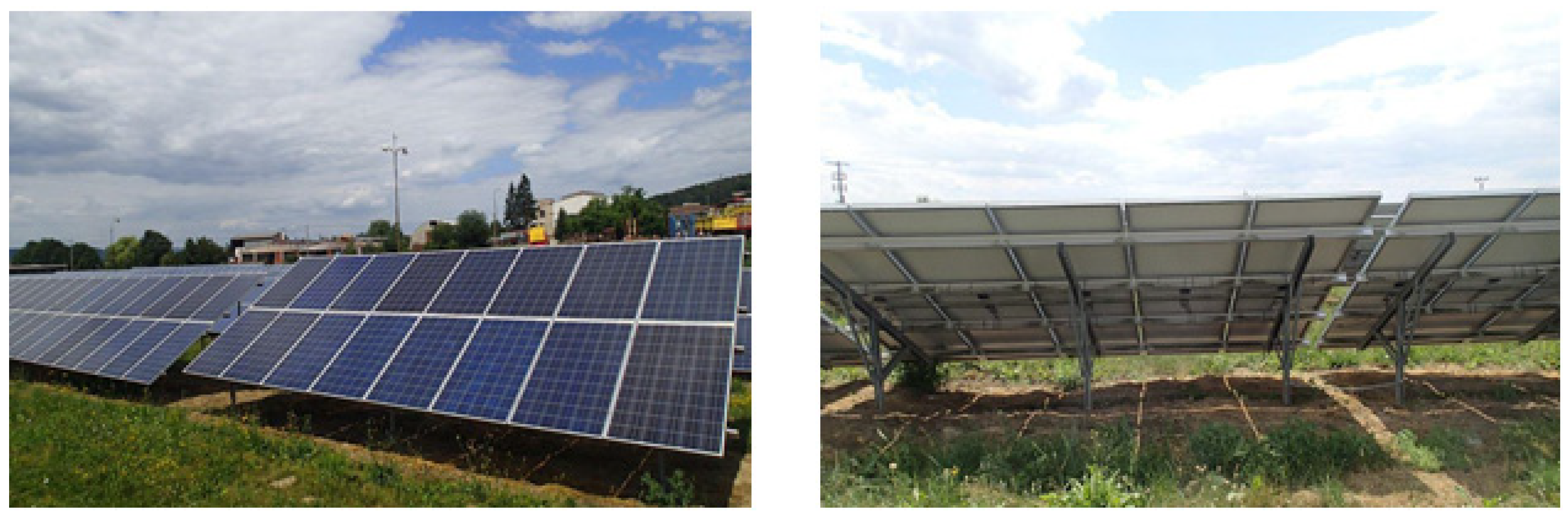
The next part describes the PV power plant and model PV system situated in the area of southern Slovakia. The monitoring of operational parameters started in January 2011 an continues today. The research was carried out during the years 2012–2019. The PV power plant is type grid on and it consists of 432 polycrystalline PV modules PHONOSOLAR PS240P−20/U (Phono Solar, Willich Germany) and the whole area of the PV system is 714.6 m² (Figure 2).

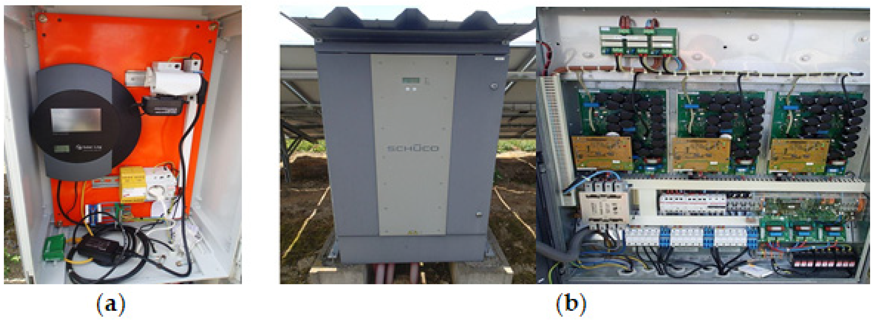
The tilt angle of PV modules is 35°, which is in the literature [2] considered to be ideal for Central Europe. The azimuth orientation of the PV modules was South with the azimuth angle 0°. Efficiency of PV module is 14.8%. Power of one PV module is 240 Wp, so the total installed power is 103.68 kWp. For converting DC voltage that is supplied by photovoltaic cells, AC voltage 230 V with frequency 50 Hz serve 3 voltage converters type Schüco Central Inverter type SGI 33 (Schüco, Prague, Czech Republic) is used. Efficiency of these converters is 97.1%. Monitoring of the PV power plant is solved using the RS485 interface, and the inverters are connected by FTP cables and monitored by Solar-Log 2000 (Solare Datensysteme GmbH, Geislingen-Binsdorf, Germany) (Figure 3). The Solar-Log 2000 offers the option to measure the amount of self-produced power consumption and it presents graphically via the Solar-Log™ WEB. The proposed system is in accordance with the technical recommendations and requirements for the interface between the PV power plant and the electrical grid according to EN 61727.

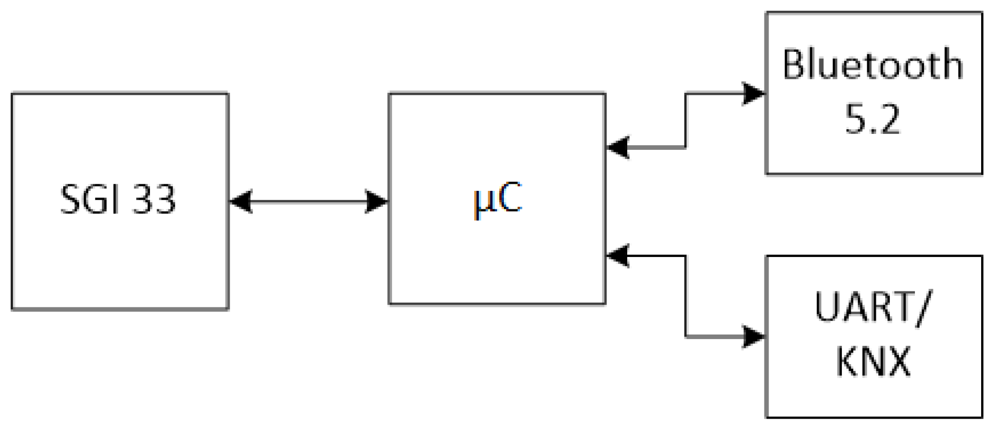
The SGI 33 inverter provides communication via the RS−485 standard. A chip with an integrated Bluetooth 5.2 radiosystem EFR32BG22C224F512GN32-C in a TQFN32 case is used in place of the microcontroller (Silicon Laboratories, Austin USA). It contains two UART modules. The first module is designed for communication with the inverter in the semi-duplex RS−485 mode with hardware flow control of the UART/RS485 converter of the MAX 481 integrated circuit. The second UART module communicates with the galvanically isolated KNX TinySerial Interface 810 and provides information on the operating parameters of the PV system with an intelligent installation element. Block scheme of communication is shown in (Figure 4).

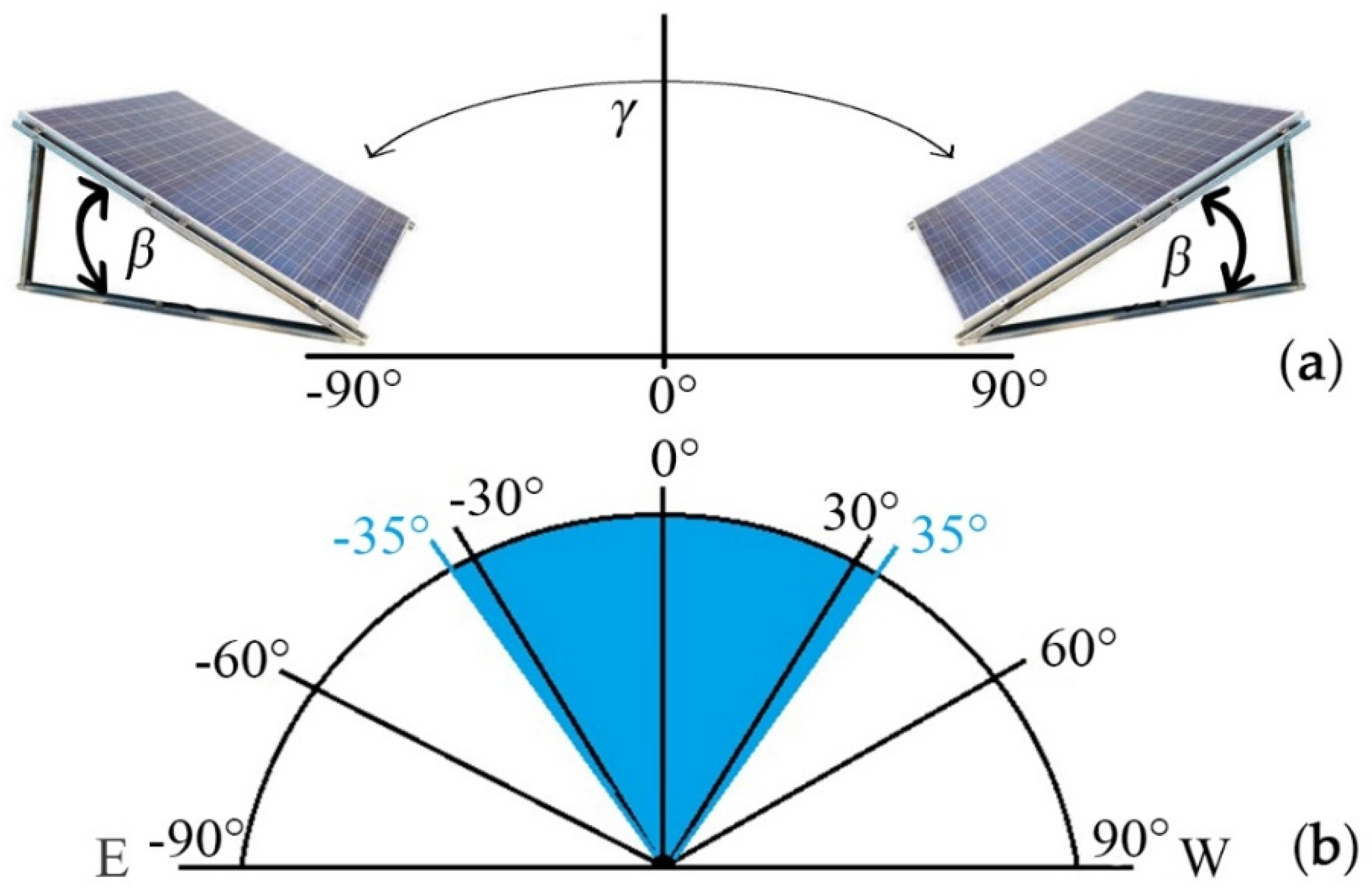
The model PV solar system was constructed from the identical polycrystalline PV module PHONOSOLAR PS240P−20/U. Each PV module was placed on a separate construction that allowed changes of the tilt angle. The operational data were collected separately for every PV module. The number of PV modules was selected according to number of different azimuth orientation represented by the azimuth angles from −90° to 90° (Figure 5). The tilt angles and azimuth angles were changed separately and manually for every PV module. The solar trackers were not used because approximately 92% of buildings have a sloping roof in southern Slovakia and non-stationary systems cannot be installed. However, roofs differ in the tilt and azimuth orientation.

The azimuth angle 0° means South, the azimuth angle +90° is West, and −90° is East. The range (−5–−85°) means Southeast (SE) orientation and azimuth angle in the range (5°–85°) means Southwest (SW) orientation of PV module (Figure 5). The results for different azimuth angles (−90°, −80°, −70°, −55°, −50°, −45°, −35°, −25°, −20°, −15°−10°, −5°, 5°, 10°, 15°, 20°, 25°, 35°, 40°, 45°, 50°, 55°, 70°, 80°, 90°) were experimentally detected by comprehensive monitoring of operational conditions (ambient temperature, temperature of PV module surfaces, intensity of solar radiation, wind speed, output electric current and voltage, output electric power, energy production). The tilt angle was changed gradually by 5°. Experimental data were collected, sorted, and numerically and statistically processed. The method of group data analysis was applied on huge data files. The time relations were detected in hourly, daily, and monthly time ranges. The measured data from the selected part model PV system (1 PV module) were compared with data from real PV power plant with the same tilt angle and azimuth angle. The results were converted to a unit of the PV module active area. The difference between each compared value was less than 0.46%. The experimental data from both PV systems with tilt angle 35° were also used for calculation of energy production. The correlation analysis confirmed 99.54% correlation between the values of energy produced by a model PV system and PV power plant.

Then were created two-dimensional graphical dependencies and by regression analysis were detected suitable mathematical equations which describe the PV system energy production as a function of tilt angle and azimuth angle. In the next step polynomial approximation on the three-dimensional graphical dependencies was performed. The verification of mathematical models was made by iteration method. In the next part the PV power plant and the model PV system are described.

Large data files were processed with spreadsheet software Microsoft Excel and Matlab^® version R2015b. All data were analysed using analysis of variance (ANOVA). The comparison of the averages was carried out by Duncan’s test with a 95% confidence level. The arithmetic averages, medians, and standard error of the arithmetic average were computed from the data. The depth data analysis and the data extraction were applied on the data files obtained from real PV system for creating a mathematical model.

3. Results

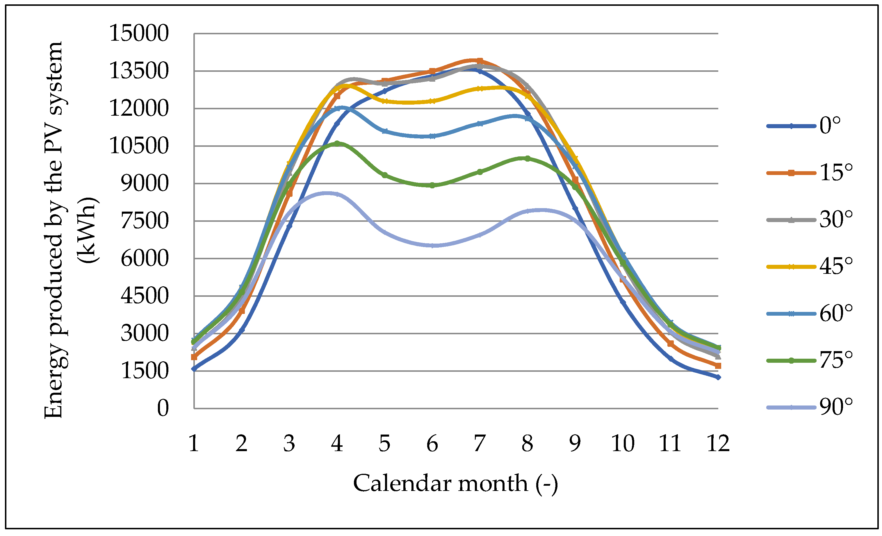
The first part of the study was focused on the identification of optimal tilt angle for southern Slovakia region. In this section the time relations for different tilt angles (0°, 15°, 30°, 45°, 60°, 75°, and 90°) were evaluated. At first, data from autonomous model solar system (1 PV module) were detected, then the results were processed and the data were recalculated on the experimental PV power plant. 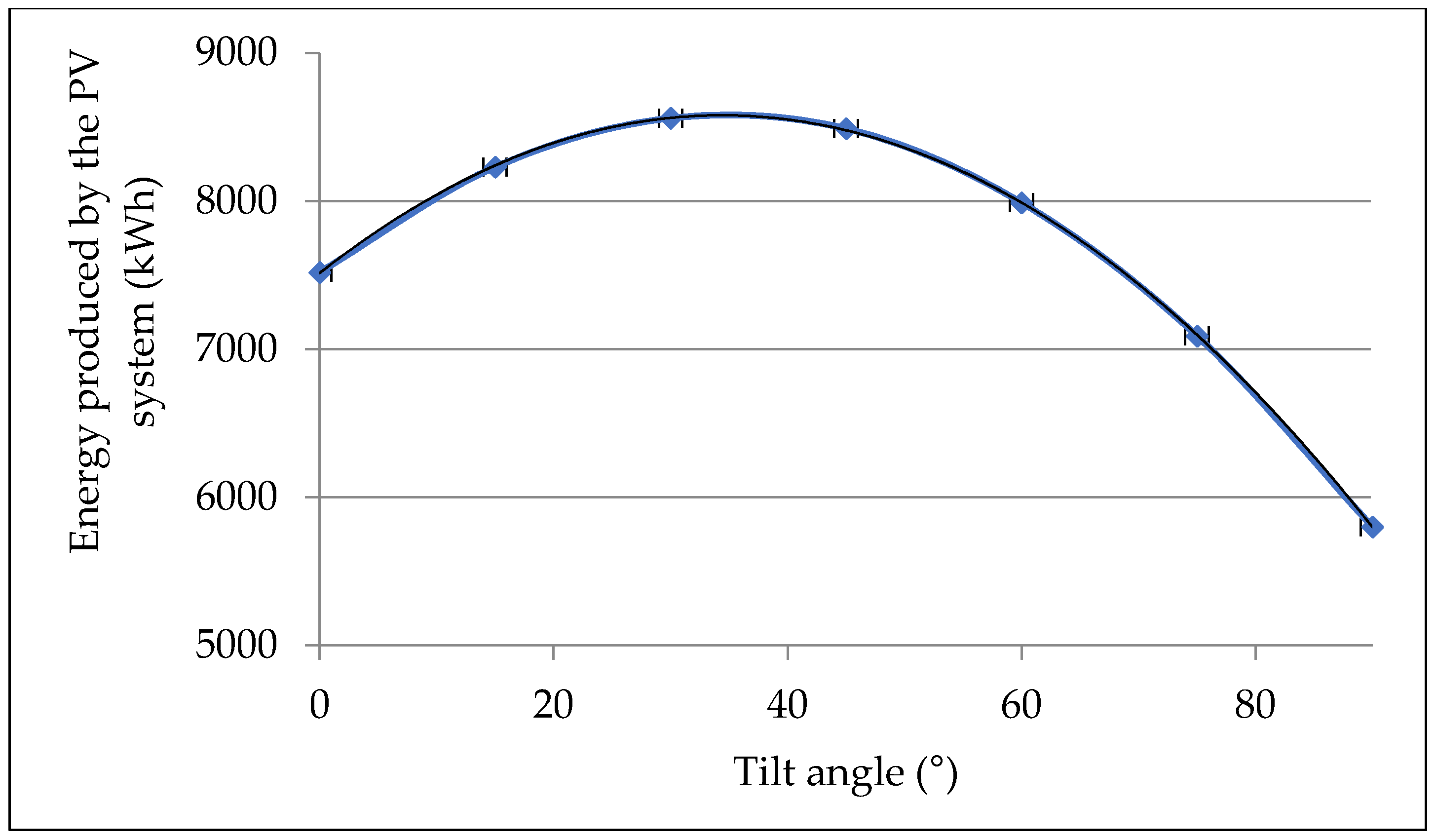The dependencies of energy produced by the PV system for tilt angle range from 0° to 90° in different calendar months are presented in Figure 6. Especially for tilt angle 35° was measured the amount of produced electrical energy not only by the model PV system but also by the PV power plant. The correlation between the calculated values and the experimentally obtained results was from 99.18% to 99.89% during the year. The output power of the system was the highest for the tilt angle 30° and the optimal energy balance was detected for tilt angle from 15° to 30°. A very small difference of about 0.9% in energy production of PV system was identified for range (30–35°). If the tilt angle is greater than the 35°, the power decreases. The group data analysis and data extraction were carried out for identifying the model equation within the observed experimental dependence. For mathematical description of power energy balance for different tilt angle β was found mathematical Equation (4), which is a polynomial function of the second degree with the coefficient of determination R² = 0.9999.

$$E_m\left(\beta \right)=-0.9{\beta }^2+61.929\beta +7514.3$$

(4)

where: $E_m\left(\beta \right)$ is the energy produced by the PV system per month (kWh), $\beta$ is the tilt angle (°). Figure 7 shows a more general relation which represents the result of the evaluation of the PV module tilt angle influence on the electricity production. The simulation in software Matlab^® was used for detection of the optimal tilt angle for examined PV system installed in southern Slovakia region. The maximum of energy production was obtained for the tilt angle 34.5°.

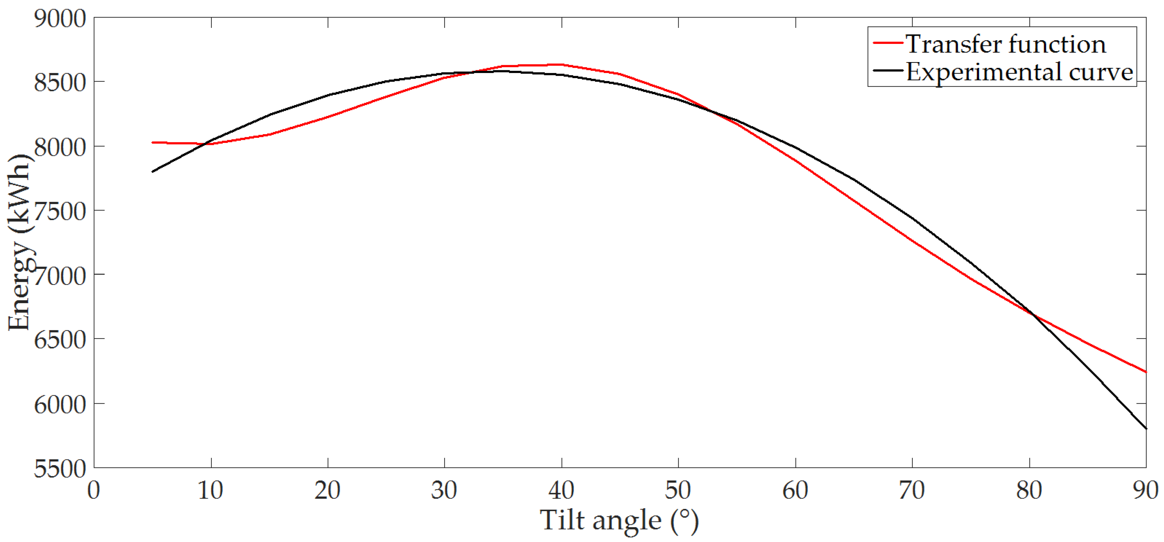
A part of the model equation verification has the polynomial function form described by Equation (4). An analytical model was created by using of iterative method for system modelling. Finally, both models (polynomial and analytical) were compared.

A 3rd order differential equation with constant coefficients—Equation (5)—was used to create the analytical model.

The differential equation describes the behavior of the output variable. From the physical point of view, it represents the amount of energy produced by the PV system, which is characterized by a transfer function in a complex plain0—Equation (6).

$$\frac{d^{3}E\left(\beta \right)}{d{\beta }^3}+0.02644·\frac{d^{2}E\left(\beta \right)}{d{\beta }^2}+0.007259·\frac{dE\left(\beta \right)}{d\beta }+5.472·{10}^{-11}·E\left(\beta \right)=-0.004562·\beta$$

(5)

$$G\left(s\right)=\frac{-0.004562}{s^3+0.02644·s^2+0.007259·s+5.472·{10}^{-11}}$$

(6)

This is based on the values of the independent variable, which was the tilt angle of PV modules β. The 95.96% reliability of the transfer function with respect to the experimental data was determined (Figure 8).

General solution of the differential Equation (7) has the form expressed as follows–Equation (7):

$$\begin{array}{c}E\left(\beta \right)=\left(7245.99·e^{-7.53823·{10}^{-9}\beta }\right)\\ +\left(e^{-0.01322\beta }·\left(-24.2152·\mathit{sin}\left(0.0841679\beta \right)+268.311·\mathit{cos}\left(0.0841679\beta \right)\right)\right)\end{array}$$

(7)

From the global extreme analysis of the model polynomial function described by Equation (6) and analytical model function—Equation (7), the global maxima of the functions were identified for the tilt angle 34,405°.

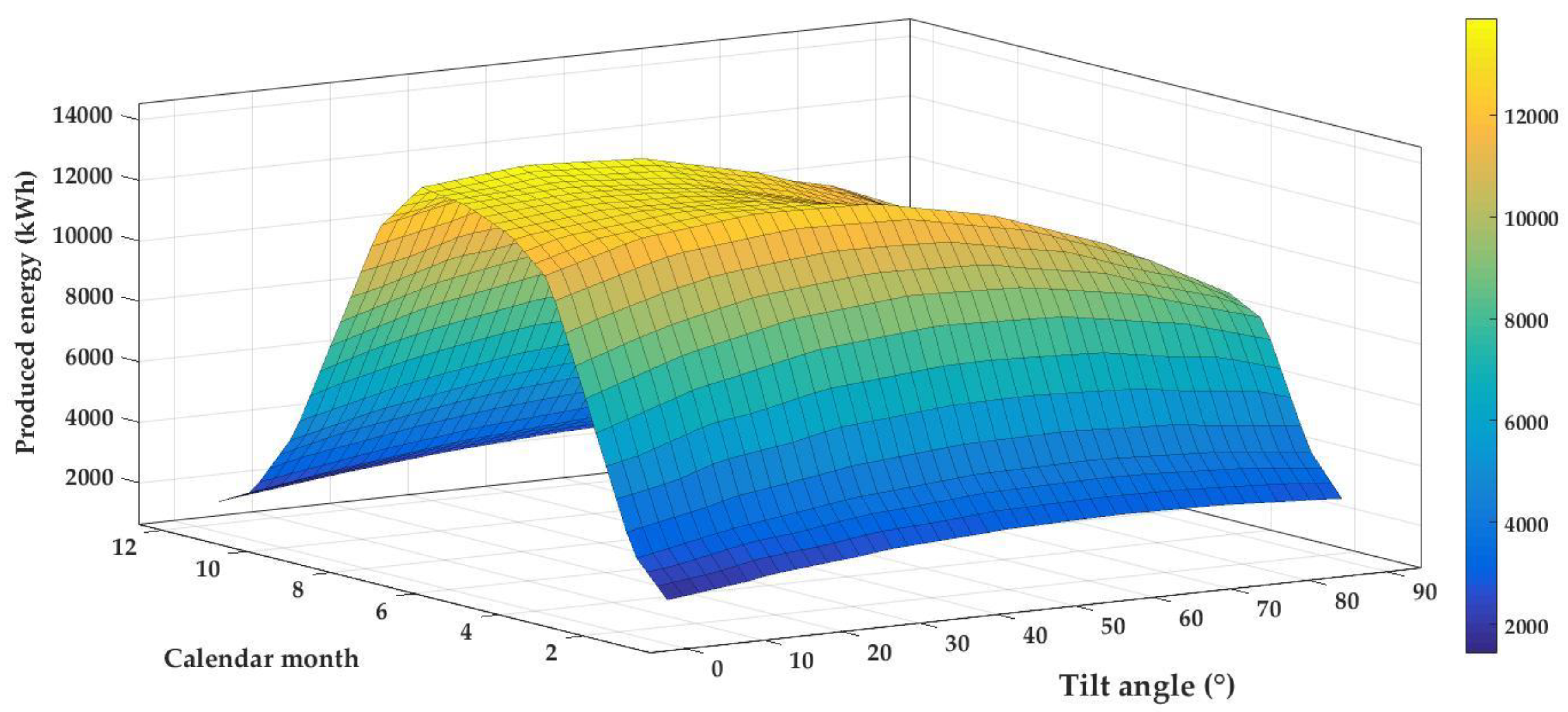
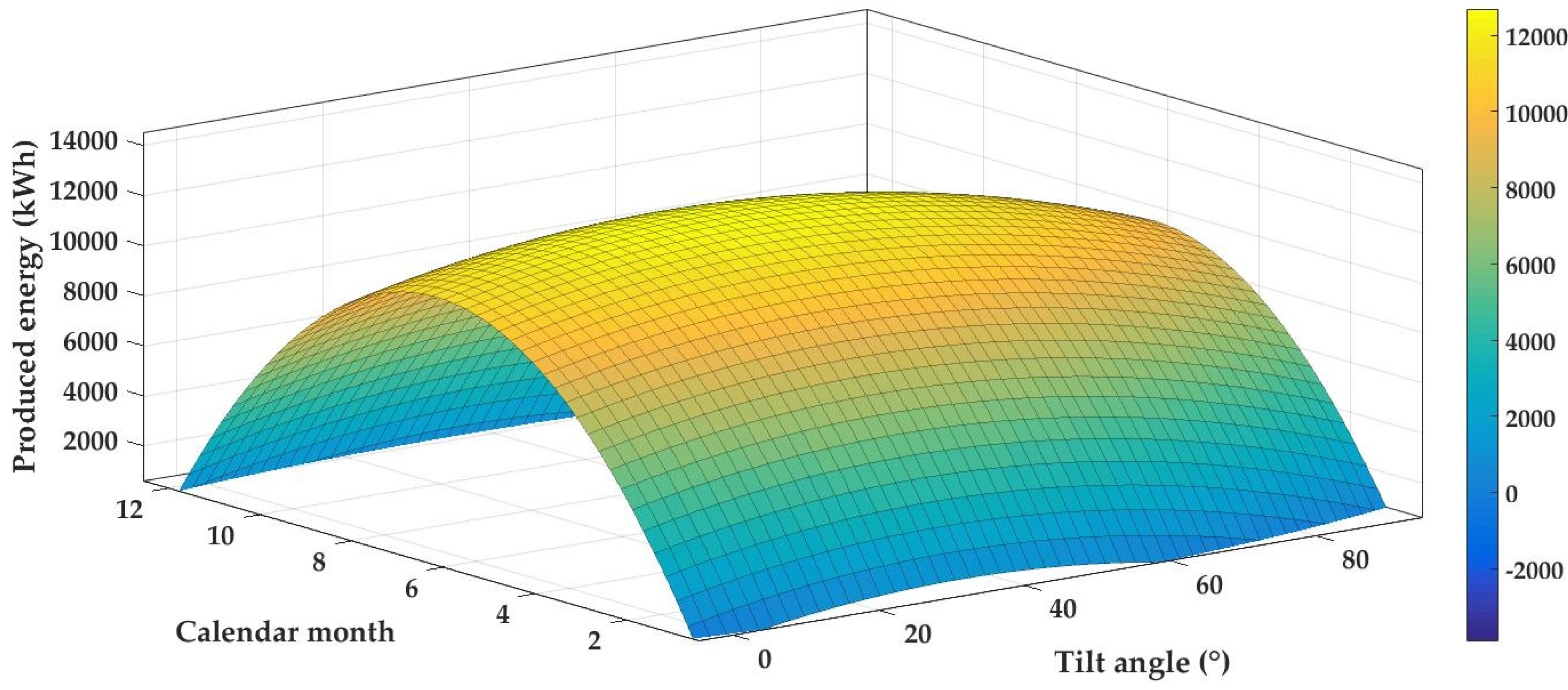
The influence of the tilt angle on the PV system electricity production during the year was also modelled by three-dimensional graphical dependence shown in Figure 9. On the presented 3D dependence was applied polynomial approximation of second degree, which was used for the x-axis and the y-axis. The x-axis shows the time represented by calendar months; the y-axis shows the individual positions of PV modules which correspond to the tilt angles. The z-axis shows the average values of the electricity produced by the PV system. The final three-dimensional model dependency is shown in Figure 10. It can be described by the characteristics which are presented in

Table 1. The statistical and regression characteristics of approximated polynomial function for three-dimensional dependence on Figure 10.

Sum of Squares	1.735 × 108
Coefficient of Determination	0.8723
Standard error of arithmeticaverage	1.491 × 103
Regression Equation	$E_m\left(t, \beta \right)=A+B·t+C·\beta +D·t^2+E·t·\beta +F· {\beta }^2$
Coefficient	Value	Minimum of the Range	Maximum of the Range
A (kWh)	−1438	−3063	−185.8
B (kWh∙month−1)	56.33	12.4	100.3
C (kWh)	4218	3785	4652
D (kWh∙month−2)	−0.8993	−1.315	−0.4835
E (kWh∙month−1)	0.8507	−2.278	3.979
F (kWh)	−340.9	−371.6	−310.2

and for mathematical description of three-dimensional relation was obtained Equation (8). The relation can be used for prediction of PV system energy balance as a function of tilt angle and month. The importance of mathematical modelling dependencies that enable the calculation of the PV system energy production was also declared by the authors [18,47,62].

$$E_m\left(t,\beta \right)=-1438+56.33·t+4218·\beta -0.8993·t^2+0.8507·t·\beta -340.9·{\beta }^2$$

(8)

where $E_m\left(t, \beta \right)$ is the energy produced by the PV system per month (kWh), $\beta$ is the tilt angle of PV system (°), and t is the time (month).

The author [2] in the publication presents that any change in the tilt angle of the PV panel is the cause of electric energy production decreasing up to 10%. Measurements on the model PV module showed the significant influence of the tilt angle, where the perpendicular placement of the PV module (90°) reduces the electricity production from 13,200 kWh to 6520 kWh, which represents 49.39%. If the tilt angle of the PV module is in the range from 0° to 30° during the months from April to August, the difference of electric energy production by PV system is minimal. Especially, the energy range was from 12,700 kWh to 13,100 kWh, which means the difference is 3.05%. However, if we compare the arithmetic average representing the energy production by the PV system in different months for different tilt angles, it is obvious that they differ from the total monthly average of 7668.571 kWh. This is especially in the range 5800–8560 kWh, which represents 24.37–11.62%. From the photovoltaic practice point of view, the average influence of the tilt angle on the energy production is approximately 18%. A considerable influence of the tilt angle is evident also from the graphical dependencies presented in Figure 6, Figure 7, Figure 9 and Figure 10. The general mathematical description of the tilt angle influence is represented by Equation (4). This equation allows the simple calculation of electric energy production by the PV system after entering the time value and the position which corresponds to the tilt angle β of the PV panel. These parameters are easy to identify in practice. Based on the model equation, it is possible to determine the energy balance of a PV plant with an installed output of 100 kWp for any tilt angle and calendar month of the year in the southern Slovakia region.

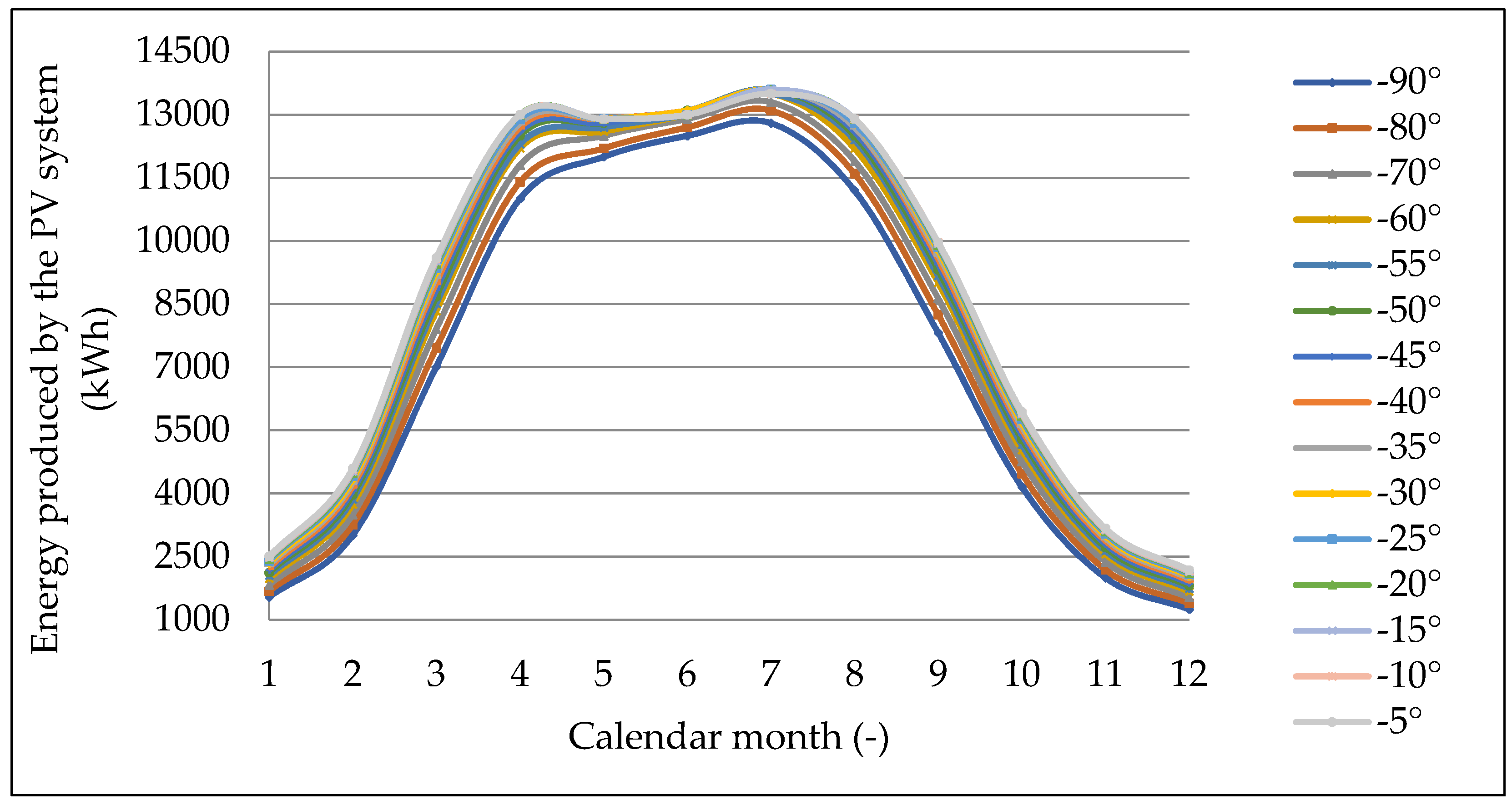
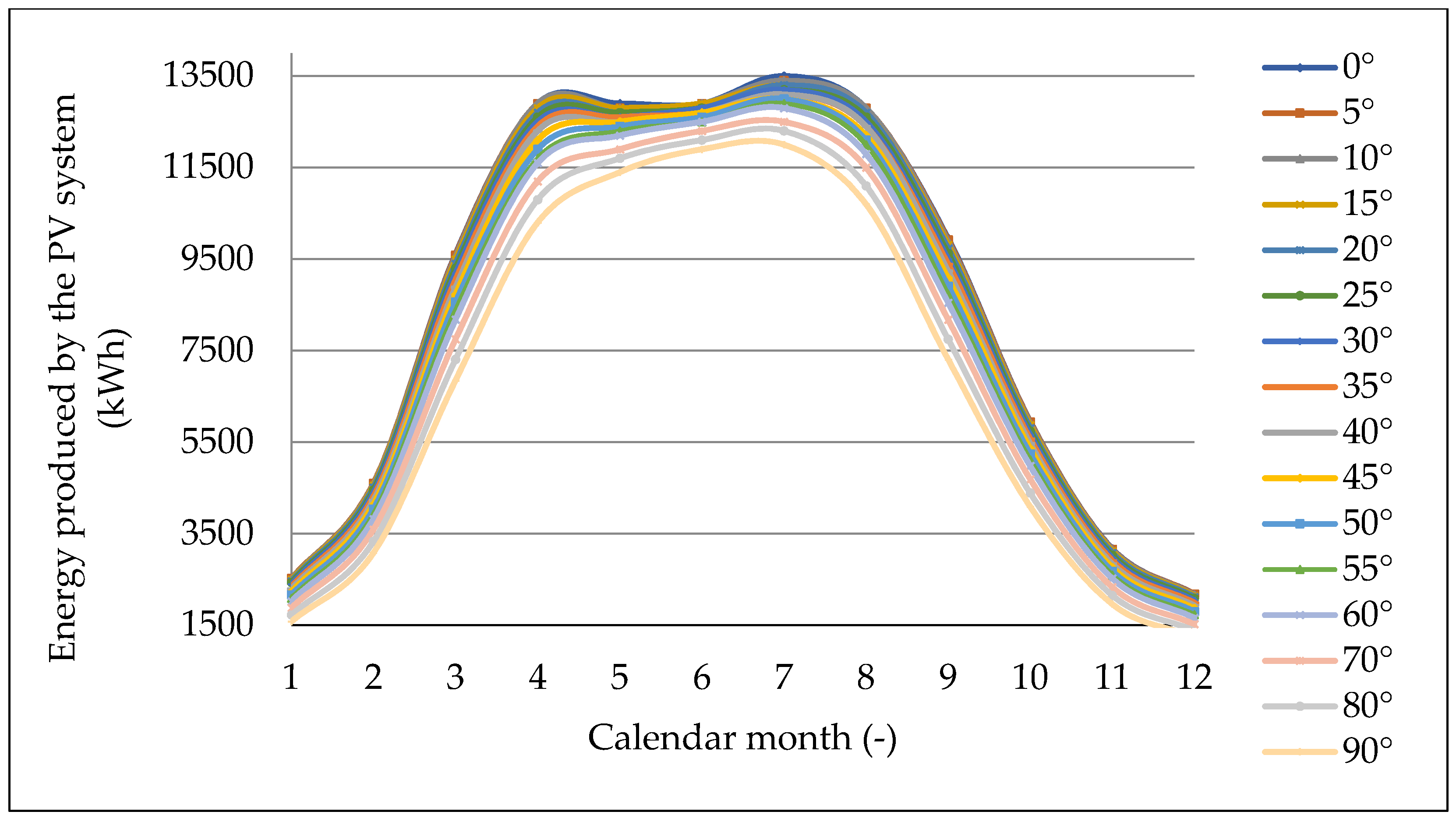
The second part of research was focused on identification of optimal azimuth angle for southern Slovakia region. Azimuth angle change was measured on PV power plant and the model PV system. The results are summarized as graphical dependencies. For clarity, results are presented in two figures. At first, dependencies were created in the range −90–5° shown in Figure 11 and then were made relations for azimuth angles 0–90° in Figure 12. The results were compared with values experimentally obtained from the model PV system for seven different azimuth orientations (−90°, −60°, −30°, 0°, 30°, 60°, and 90°). The difference between values obtained from the PV power plant and model PV system was approximately 0.58%.

The measured data were statistically processed and the selected statistical characteristics for each data group were calculated. Especially, arithmetic average, deviations from arithmetic average, variance σ², standard deviations σ, standard error of arithmetic average $\overline{\mathsf{\delta }}$(t), and the median were identified. Selected summary results are presented in

Table 2. Average amount of energy ($\overline{E}$ ) produced by PV system with different azimuth orientation and tilt angle 35°, average energy produced per month (${\overline{E}}_m$ ).

Azimuth angle	−90°	−80°	−70°	−60°	−55°	−50°	−45°	−40°	−35°	−30°	−25°
$\overline{E}$ (kWh)	7190	7480	7750	7990	8090	8190	8280	8350	8420	8470	8520
Median (kWh)	7415	7855	8275	8670	8840	8995	9150	9290	9415	9525	9605
Azimuth angle	−20°	−15°	−10°	−5°	0°	5°	10°	15°	20°	25°	30°
$\overline{E}$ (kWh)	8560	8580	8590	8590	8580	8560	8540	8500	8450	8380	8310
Median (kWh)	9675	9730	9775	9785	9780	9755	9715	9650	9565	9460	9345
Azimuth angle	35°	40°	45°	50°	55°	60°	70°	80°	90°
$\overline{E}$ (kWh)	8230	8150	8050	7950	7830	7710	7450	7170	6870
Median (kWh)	9220	9065	8905	8735	8555	8365	7965	7530	7080
Month		January	February		March		April		May	June
${\overline{E}}_m$ (kWh)		2200.32	4094.19		8758.71		12280.65		12567.74	12793.55
$\overline{\mathsf{\delta }}$(P) (kWh)		52.38	84.16		143.67		129.42		69.67	52.78
Month		July	August		September		October		November	December
${\overline{E}}_m$ (kWh)		13225.81	12325.81		9221.29		5361.61		2778.71	1868.39
$\overline{\mathsf{\delta }}$(P) (kWh)		72.67	104.48		101.07		97.96		64.6	51.17

.

Summary results for energy produced by PV system with different azimuth orientation are presented in

Table 3. The statistical and regression characteristics of approximated polynomial function for three-dimensional dependence in Figure 14.

Sum of Squares	4.975 × 108
Coefficient of Determination	0.9314
Standard error of arithmetic average	1.1680 × 103
Regression equation	$E_m\left(t, \gamma \right)=A+B·t+C·\gamma +\mathrm{D}· t^2+E·t·\gamma +F {\gamma }^2$
Coefficient	Value	Minimum of the Range	Minimum of the Range
A (kWh)	−2215	−2656
B (kWh∙month−1)	−2.104	−7.389	3.18
C (kWh)	4965	4815	5116
D (kWh∙month−2)	−0.1949	−0.2453	−0.1446
E (kWh∙month−1)	−0.009663	−0.7277	0.7084
F (kWh)	−396.7	−408	−385.4

. It is clear that the largest amount of electrical energy is produced for the azimuth orientation from −5° to −35°, which represents the energy range (8420–8590) kWh. In the South orientation 0°, the PV system produced 8580 kWh. In the Southwest orientation was the maximum energy production in range 8560–8450 kWh obtained for azimuth angles from +5° to +20°.

The comprehensive evaluation of the results for the azimuth angle that influenced the PV system energy production pointed to the fact that optimum energy is achieved at the azimuth angle −20–15°. However, the average difference is only 3.80% as compared with the orientation in the range (−35–35°), which is presented as acceptable for the azimuth angle for the PV module orientation in literature [16,63,64,65].

From the results interpretation of the azimuth angle changes simulation on the PV system energy production, it is clear that the time is one of the most important factors. The amount of energy produced by the PV system varies from month to month when changing the azimuth angle of rotation from −90° to +90°. The extensive data set will assess the impact in selected model months of the relevant season. The largest amount of electricity is produced in the summer months, specifically in July, where for the above azimuth angle range, the PV system is produced at least 12,000 kWh at +90° orientation and 13,600 kWh at azimuth angle from (−50–15°). It means change of energy production 11.76% in relation to the maximum energy production in July. It follows from the above facts that in the summer months the influence of the azimuth angle is minimal and the changes in the amount of produced energy is on average 12.18%. After analyses of the energy production during the winter months in a similar way, the amount of produced energy in January was 1580 kWh for the azimuth angle +90° to 2520 kWh at the azimuth angle in range (0–5°). It means change of 37.30% from the maximum energy production in January. The influence of the azimuth angle changes in winter is on average 36.55%. It can be compensated for example by optimizing of the PV module tilt angle. From the spring months typical March is the model month, where the amount of produced energy was (6850–9610) kWh; the change in the amount of produced energy in March was affected by an azimuth angle of 28.72%. Minimum energy production was reached in March with azimuth orientation of +90° and maximum energy production with azimuth orientation of 0°. Numerically, the effect of the azimuth orientation changes on energy production is during the spring 19.38%. Similarly, model autumn month October was analysed. The minimum energy production during October was 4090 kWh at +90° and the maximum energy production was 5950 kWh for azimuth orientation 0°. The difference in October was 31.26%, and the average change of energy balance was 31.51% in the autumn season.

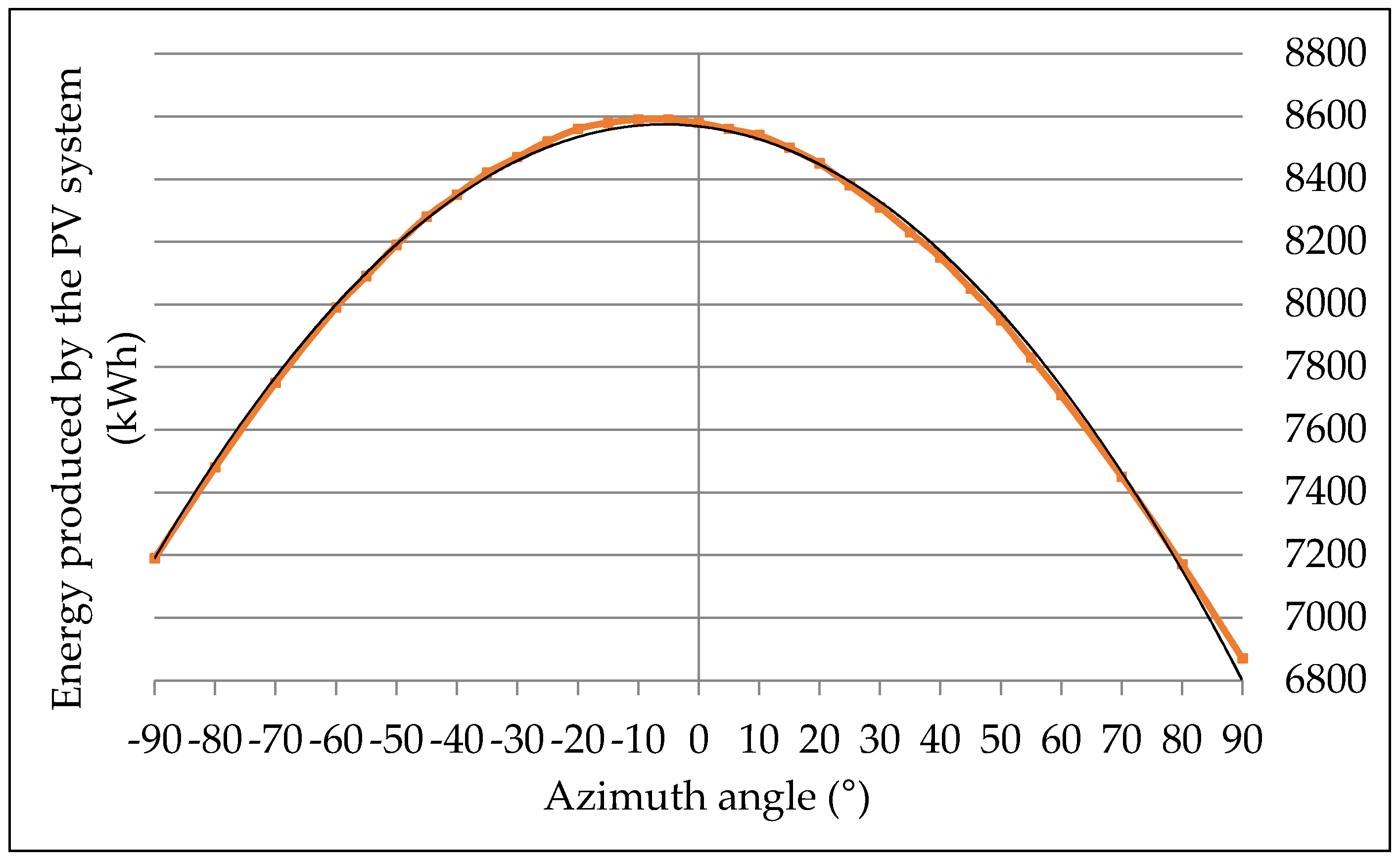
The presented results show that in terms of the energy balance, the maximal production was achieved for azimuth angle from −5° to −10° Southeast when the average energy production was 8590 kWh. More generally, the assessment of the effect of the PV module azimuth angle on the amount of produced energy is shown in Figure 13. The final observed dependence can be described by the regression Equation (9). It represents the polynomial function of the second degree with the coefficient of determination R² = 0.998.

$$E_m\left(\gamma \right)=-0.1943·{\gamma }^2-2.1746·\gamma +8568.8$$

(9)

where $E_m\left(\gamma \right)$ is the energy produced by the PV system per month (kWh) and $\gamma$ is the azimuth angle (°).

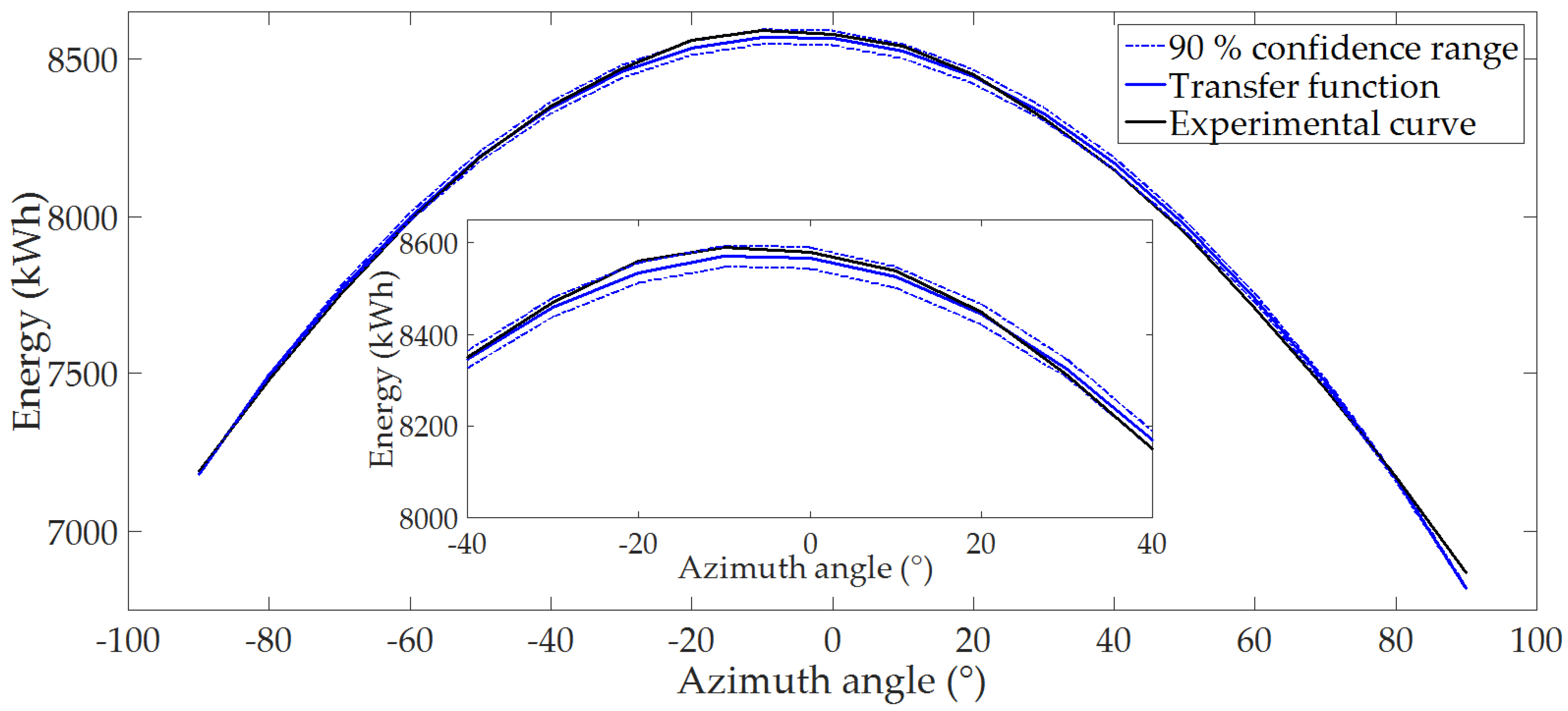
In the case of Figure 13, a purely parabolic trend of functional dependence was detected. Within the analytical model, the first order differential equation with constant coefficients—Equation (10)—was compiled. As in the previous analytical solution, a transfer function in a complex plain described by Equation (11) was used and subsequently a general solution of the differential Equation (10) was found. The coefficient of determination for the transfer function—Equation (11)—was 96.25%,

$$\frac{dE\left(\gamma \right)}{d\gamma }+490.3·{10}^{-6}·E\left(\gamma \right)=-0.3879·\gamma$$

(10)

$$G\left(s\right)=\frac{-0.3879}{s+0.0004903}$$

(11)

where γ is the azimuth angle (°). From the mathematical description of the parabolic course by polynomial function of the second degree, it is possible to determine the position of the stationary point, which corresponds to an azimuth angle of −5.60°. Due to the information known from PV theory, a calculation was performed for the azimuth angle γ = 0°. The general solution of the differential Equation (10) for the mentioned azimuth angle γ can be expressed in the form of Equation (12):

$$E\left(\gamma \right)=8568.8·e^{-0.0004903\gamma }$$

(12)

A comparison of the analytical model results with functional dependence is shown on Figure 14.

Matlab^® version R 2015a was used for the mathematical model creation. Three-dimensional dependencies were created by mathematical software. The suitable polynomial approximation was applied to the relation of data files. For the three-dimensional relation, selected statistical parameters and regression coefficients of Equation (13) were calculated, which are summarized in Table 3.

$$E_m\left(t,\gamma \right)=-3603+4966·t+192.6·\gamma -396.7·t^2-0.05377·t·\gamma -6.372{\gamma }^2$$

(13)

where $E_m\left(t, \gamma \right)$ is the energy produced by the PV system per month (kWh), γ is azimuth angle (°), and t is the time (month).

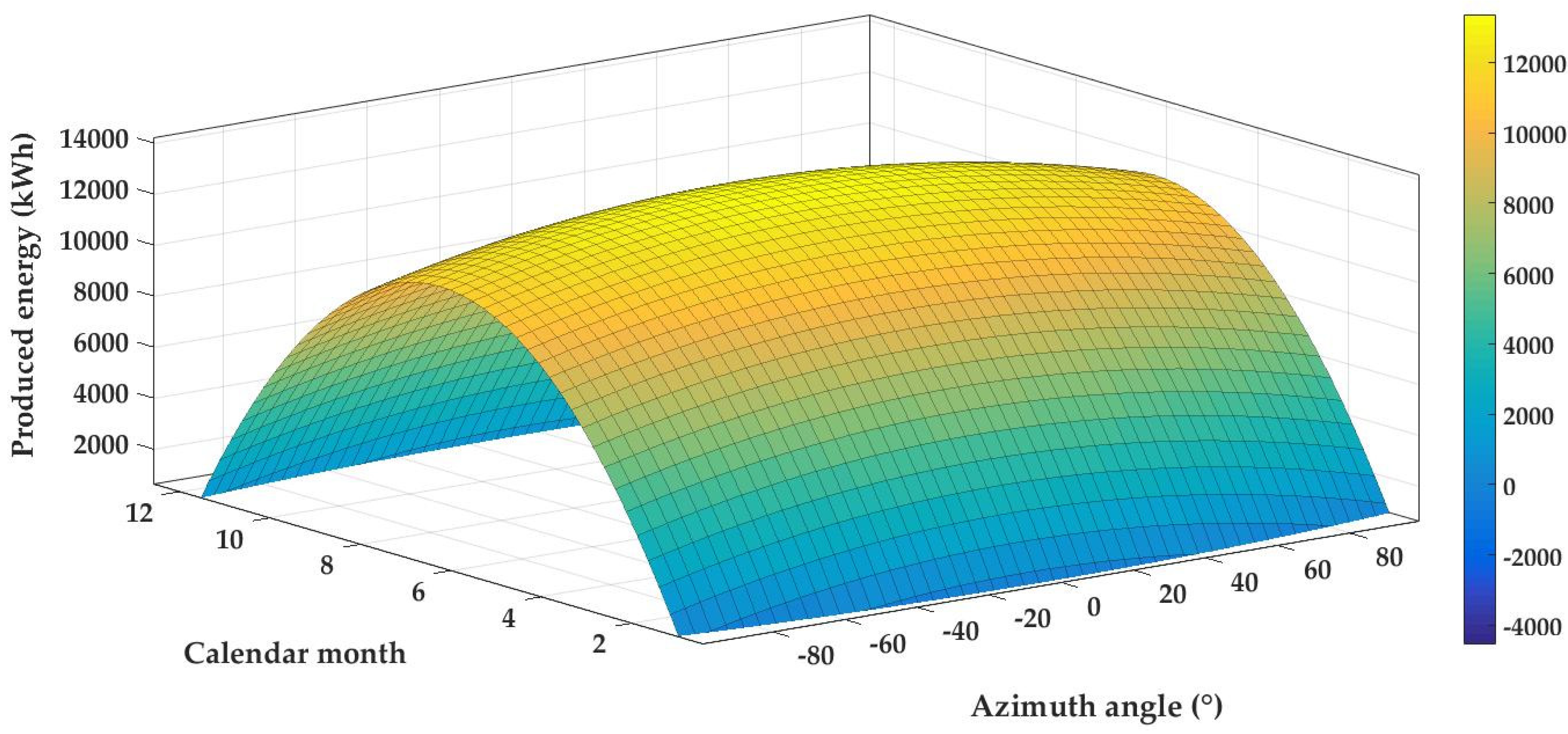
The final relation for the influence of the azimuth angle on the amount of produced energy by the PV system can be modelled by using three-dimensional graphical dependence, which is shown in Figure 15. The x-axis shows the time represented by calendar months and the y-axis represents the positions which correspond to the azimuth angle of PV module. On the z-axis are plotted average values of produced energy.

4. Discussion

The research results can be divided into two parts. In the first part the effect of the tilt angle changes will be discussed. The second part of presented research aimed to determine the influence of the azimuth orientation on the resulting energy balance of the PV system. The results mentioned in the previous chapter take into account not only experimental data but also mathematical models which were created. The mathematical evaluation of the final function relations was done by software Matlab^®.

The polynomial function pointed to the fact that the tilt angle 34.5° is the best for PV module installed in the southern Slovakia region. The obtained result was verified by analytical model, which confirmed that optimal tilt angle of PV module installed in the Southern Slovakia regions is 34,405°, which agrees with the result calculated by using the model polynomial equation. The tilt angle difference between models was 0.095°. Presented results are also in good agreement with the information presented in literature [65] and values of energy production amounts for every month are consistent with the results reported by research in the articles [20,21].

From numerical assessment of results for azimuth angle orientation in the southern Slovakia, it is evident that maximal power and energy production of PV system was obtained for azimuth angle in the range (−20–15°). This fact is in agreement with information presented in the literature [66], but the best energy production is detected if the azimuth angle is −5°, which means the South-East orientation. The average energy losses if the PV modules have South (0°) azimuth orientation were 0.12%. The fact is known also from the literature [13] where general information is presented. Our research confirmed significant influence of azimuth angle and tilt angle on PV system energy production, which is in accordance with results presented by authors [11,17,27,37,53,56].

For verification and evaluation of the experimental results and the created mathematical models special photovoltaic software was also used, which enabled the simulation of the operating conditions of the PV system for the selected area. In this software the simulation of solar radiation and PV system energy production was performed. Software calculates the solar radiation from satellite according to the methodology described in publications [62,63,64]. The calculation of PV system power is based on Equation (14),

$$P=\frac{G}{1000} ·A·eff\left(I_G,T_m\right)$$

(14)

where P is power of PV module (W), I_G is solar radiation (W.m⁻²), A is area of PV system (m²), eff is efficiency of PV system (%), and T_m is temperature of PV module (°C) [62]. The total amount of energy PV system production was identified as a product of the PV system power by using Equation (14) and selected time range.

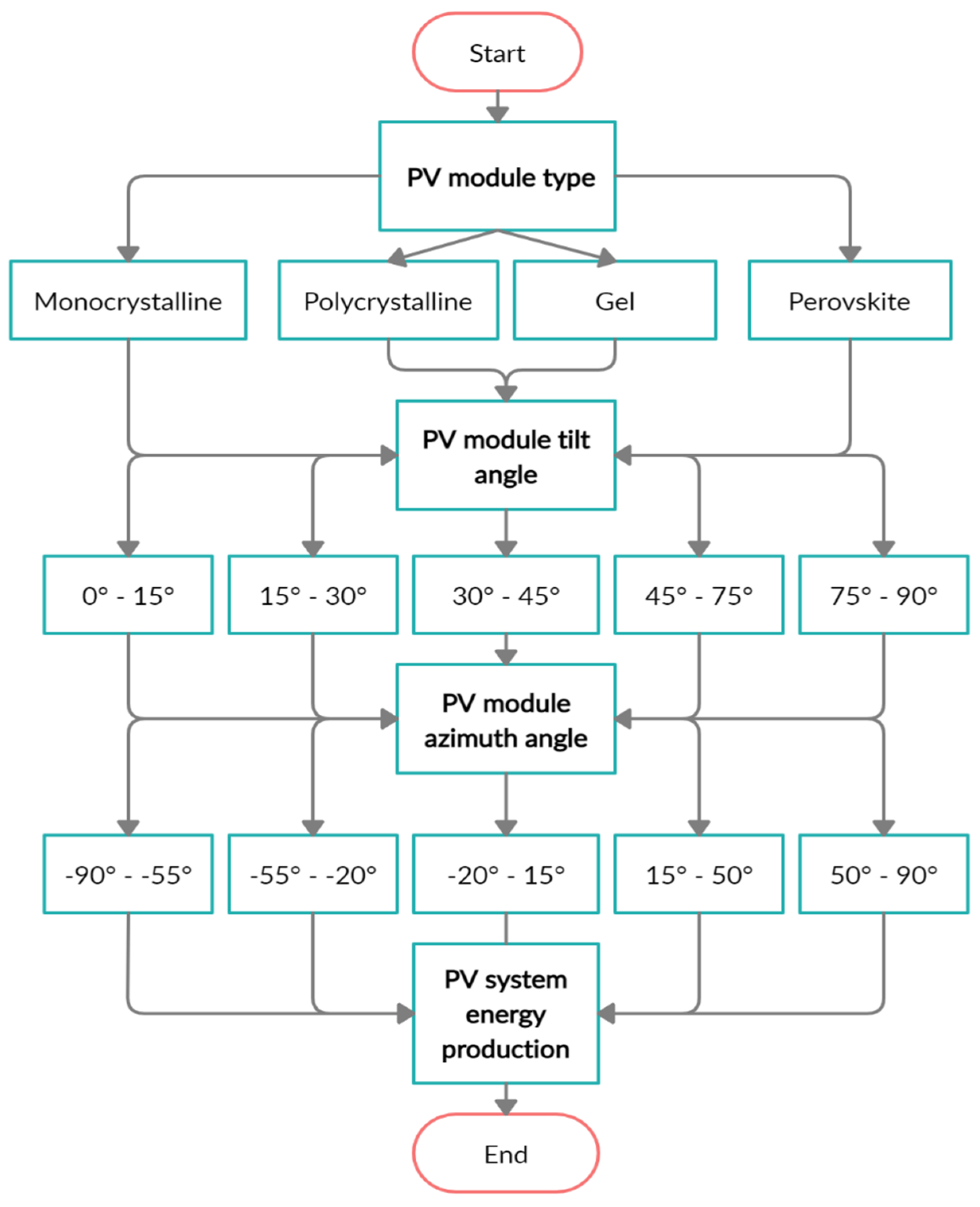
The dependencies found in the experimental work were summarized and made a contribution to a comprehensive basis for the creation of a final mathematical model. The final model will be a platform for creation of smart application. Part of the flowchart is presented in Figure 16. Due to the applicability of the mathematical model in practice and the possibility of its use by the target group, which will be ordinary users, the model had to be simplified. It contains easily identifiable parameters. The created mathematical model allows for the prediction of power or energy of a PV system installed in southern Slovakia region. The equation for the simplified performance model has the form described by Equation (15):

$$P\left(t\right)=k_{type}·k_{const}·k_{tilt}·k_{azim}·k_{tcell}·k_{loss}·f_G\left(t\right)·P_{inst}$$

(15)

where P is power of PV system in kW, k_type coefficient for PV module type, k_const is coefficient for PV system construction, k_tilt coefficient for PV module tilt angle, k_azim is coefficient for PV module azimuth angle, k_tcell is coefficient for PV cell temperature, k_loss coefficient for PV system loss, f_G(t) is the function for solar radiation intensity in kW∙m⁻², and P_inst is installed power of PV system in kW_p.

The tilt angle of PV panels in relation to the location and azimuth position was investigated experimentally in many studies. Latitude based model for tilt angle optimization for solar systems in the Mediterranean region was detected by [67]. Mentioned article presents also quadratic regression model that allows the prediction of the annual optimal tilt angle. Optimum tilt angle for 1 MW PV system at Sukkur in Pakistan was determined and described in literature [68]. The research results confirmed the tilt angle variations during the year from 0° to 61.1° in the northern Pakistan. It was found that optimal tilt angle for that region is 29.5°. An experimental and mathematical investigation of optimal tilt angle and effects of reflectors on PV energy production was presented by authors [69]. Experimental results show that for gain of optimum power output the tilt angle needs to be changed every month. From experimental study located in Nitte (India), it was found that the PV system produced maximum power output in April for tilt angle 0°; in March optimal tilt angle is 13°, for February 22°, tilt angle for January is 33° and 30° for December. World estimates of PV optimal tilt angles and ratios of sunlight incident upon tilted and tracked PV panels relative to horizontal panels were described in [70].

One of the best ways to optimize the energy balance of PV panels is to use solar trackers that can optimize their position. The use of solar trackers can increase electricity production by around a third, and some claim by as much as 40% in some regions, compared with modules at a fixed angle. In any solar application, the conversion efficiency is improved when the modules are continually adjusted to the optimum angle as the sun traverses the sky. As improved efficiency means improved yield, use of trackers can make quite a difference to the income from a large plant. This is why utility scale solar installations are increasingly being mounted on tracking systems [71]. One of the best technologies for PV module position optimalization are dual axis trackers. Dual axis trackers typically have modules oriented parallel to the secondary axis of rotation. No matter where the Sun is in the sky, dual axis trackers are able to angle themselves to be in direct contact with the Sun [72]. Very innovative idea is presented in literature [51] where authors described design and performance of a new self-powered LCPV solar trackers using bifacial solar cells and concentrating mirror. All mentioned references confirmed that the orientation of the module with respect to the tracker axis is important when modelling performance. However, when installing solar trackers, there are design and economic limitations that do not allow their use. In this case, it is essential to install a PV system with fixed panels into the best operating position and it is appropriate to use the created mathematical model.

All the above mentioned publications confirm the local variability of the PV panels tilt angle and azimuth orientation. It is in accordance with the results presented in the text. It should be emphasized that the effect of both angle changes on energy production in Central Europe was declared by other experimental results which were obtained during the several years in Czech Republic, specifically in the region of Brno and Prague. Identical methods of processing and evaluation of experimental data were used. It was found that in the region of Nitra in Slovakia the optimal angle of inclination is 34.5°, in the region of Brno in the Czech Republic it is 34.7°, and in the region of Prague the optimal tilt angle is 35°.

5. Conclusions

From the presented results it is a clear well-known fact that the tilt angle and azimuth angle have significant influence on the total energy balance of the PV system. The research also confirmed that is very important to know the optimal tilt angle and azimuth angle orientation for the area in which the PV system is installed. The first benefit of presented research is a simplified mathematical model for energy production expressed through the time relations for tilt angle and azimuth angle which contains a very small number of input parameters which are easily identifiable to ordinary users of PV system. The results of the research presented in the manuscript are localized to the area of Southern Slovakia, but the general forms of model equations are applicable to the area of Central Europe respectively for areas with similar climatic conditions. For a detailed prediction of energy production in certain areas, a modification of regression equation coefficients and differential equations can be applied. The second benefit is that the model can be described by the simple polynomial function of the second degree. Since the model equations were created on the basis of data processing from long-term monitoring of the operating parameters of the PV system, the resulting model, although not based on data obtained by satellite measurements, gives results better corresponding to the real energy production of the PV system at the site. The third benefit is that the mentioned mathematical model gives about 4% more accurate results than models used so far for the locality of southern Slovakia. Experimental methods, numerical simulation, and data analysis find that the effect of PV module tilt angle on the amount of electricity generated by the PV power plant is about 18%. The ideal tilt angle for southern Slovakia region is 34.5°. The effect of azimuth angle changes on the PV system energy production is 24.19% during the year. Maximum energy production was achieved in the selected locality at azimuth angle from the range (−20–15°). All obtained results are a part of final mathematical model for simulation of PV system power and energy balance. This model created the platform for development of application for smart devices. Presented results allow a simple prediction of the energy production of a PV power plant installed in real operating conditions and they can be used in practice for the design, dimensioning, and optimization of PV power plants in the southern Slovakia.