Keyboard Model of Seismic Cycle of Great Earthquakes in Subduction Zones: Simulation Results and Further Generalization

Abstract

Catastrophic megaearthquakes (M > 8) occurring in the subduction zones are among the most devastating hazards on the planet. In this paper we discuss the seismic cycles of the megathrust earthquakes and propose a blockwise geomechanical model explaining certain features of the stress-deformation cycle revealed in recent decades from seismological and satellite geodesy (GNSS) observations. Starting with an overview of the so-called keyboard model of the seismic cycle by L. Lobkovsky, we outline mathematical formalism describing the motion of seismogenic block system assuming viscous rheology beneath and between the neighboring elastic blocks sitting on top of the subducting slab. By summarizing the GNSS-based evidence from our previous studies concerning the transient motions associated with the 2006–2007 Simushir earthquakes, 2010 Maule earthquake, and 2011 Tohoku earthquake, we demonstrate that those data support the keyboard model and reveal specific effect of the postseismic oceanward motion. However, since the seismogenic blocks in subduction systems are mostly located offshore, the direct analysis of GNSS-measured displacements and velocities is hardly possible in terms of the original keyboard model. Hence, the generalized two-segment keyboard model is introduced, containing both frontal offshore blocks and rear onshore blocks, which allows for direct interpretation of the onshore-collected GNSS data. We present a numerical computation scheme and a series of simulated data, which exhibits the consistency with measured motions and enables estimating the seismic cycle characteristics, important for the long-term earthquake forecasting.

1. Introduction

Large-magnitude subduction-associated earthquakes with M > 8 cause the release of enormous elastic stresses accumulated over hundreds of years or even a millennium. Forecast of such shocks, leading to substantial social, economic and ecological consequences, is one of the most crucial problems in geophysics [1,2]. To date, the most developed forecast-related approaches include deformational monitoring [3,4,5], identification of geophysical precursors, as well as statistical analysis of the seismicity pattern [6,7,8]. Machine learning (ML) techniques and big data analysis have also become a trend in recent years, and have potential to increase forecast reliability [9]. However, given the rare occurrence of catastrophic M > 8 events (around once-in-a-century), with only few such megaearthquakes recorded over a history of seismological observation, this approach is faced with difficulties due to a small size of the training sample. Thus, some physical (mechanical) model is strongly needed for appropriate description of geodynamical setting during the earthquake preparation phase, and such model might be employed in combination with ML methods to better constrain the results.

Geomechanical models used in seismology and geodynamics are mainly based on continuum mechanics, and widely employ the concept of the continuous structure being ruptured at the instant of an earthquake which results in the formation of a plane fault [10,11]. Models of seismic cycles associated with the strongest subduction earthquakes are mostly based on the concepts of the widely used “asperity” model [12], which explains the difference in characteristic sizes of sources and recurrence periods of catastrophic earthquakes in various subduction zones. Later, a set of mechanical models describing the generation of strongest earthquakes with the source length up to 1000 km was proposed assuming the idea of synchronous failure of several adjacent asperities: from a first simple model [3] to a very complex model by [4,5]. An explanation of seismic–aseismic slip patterns observed on megathrust faults proposed in [13] is also worth mentioning: the results of numerical simulations based on the quasi-dynamic asperity fault model with the slip-dependent friction and stress-dependent healing quite accurately reproduces the main features of real megathrust fault behavior.

However, this approach is still lacking accuracy when modeling the processes of the earthquake preparation, stress release, and post-quake stress relaxation. Analysis of the large-magnitude tsunamigenic earthquakes and seismotectonic features of various subduction zones suggests that these regions have essentially a fault-block structure, with certain patterns in their kinematics [14,15]. The studies based on GPS-measured displacements of the Earth’s surface in the source areas of large recent earthquakes during different stages of the seismic cycle, have also confirmed the fault-block structure in the frontal part of the continental margin [16,17,18,19]. Thus, geodetic observations combined with geological and seismological studies, clearly indicate that the continental lithosphere in subduction regions has complex structure, revealing a number of separate blocks which move independently from each other.

Explanation of the observed displacements and velocities, which sometimes have opposite direction in neighboring blocks, is hardly possible in terms of the well-known asperity model [12]. At the same time, interpretation of this motion pattern might be possible assuming the so-called “keyboard” model proposed by Lobkovsky et al. [20]. This concept is essentially a geomechanical model describing seismotectonic evolution of subduction regions, taking into account the fault-block structure of the continental margin. Application of the above model implies identification of large fault-separated blocks in the considered area based on geological, geophysical, seismological and geodetic data, which allows tracing their lateral boundaries.

The model involves a numerical formalism allowing for simulation of the displacements of frontal seismically-active blocks in the subduction zone during different phases of the seismic cycle, assuming that rear portion of the continental lithosphere (which corresponds to island arc) is a single structural element that is not separated into smaller blocks and does not experience its own horizontal displacements. However, the GPS-measured velocities along with geological and seismological data clearly indicate that the structure in the rear part of the subduction region also consists of separate segments divided by large faults rooted into the contact zone of interacting lithospheric plates [18,21].

Due to the relatively weak interaction between neighboring blocks, each of them can deform nearly independently of adjacent structural segments, while the overall deformation of the entire system may exhibit a very complex pattern. During seismic events, the rear blocks, similar to frontal ones, may experience almost instantaneous offsets towards the trench. Once the stress is released, a slow straightening of the rear blocks occurs in the postseismic period, partly restrained by the viscous friction at the bottom of the block due to the underlying asthenospheric layer.

The above considerations indicate the need for modification of the original model [20] in order to take into account the discontinuities both in the frontal and rear parts of the island arc. An important motivation for model improvement is also the fact that geodetic observations of Earth’s surface motions are mainly carried out onshore, that is, within the rear segment of subduction system, which troubles the direct interpretation of the available displacement data within the framework of the original single-segment model.

A very brief analysis of the generalized model has been published in [22]. In this paper, we discuss the motivation for application of keyboard model in order to explain observed motion patterns in subduction regions, with primary focus on its generalization, leading to the modified two-segment keyboard model. We also present some preliminary simulation data calculated assuming elastic spring-like interaction between the frontal and rear segments.

2. Materials and Methods

In this section we provide the description of single-segment keyboard model and then discuss the observational GNSS evidence and reasoning for the necessity of model generalization.

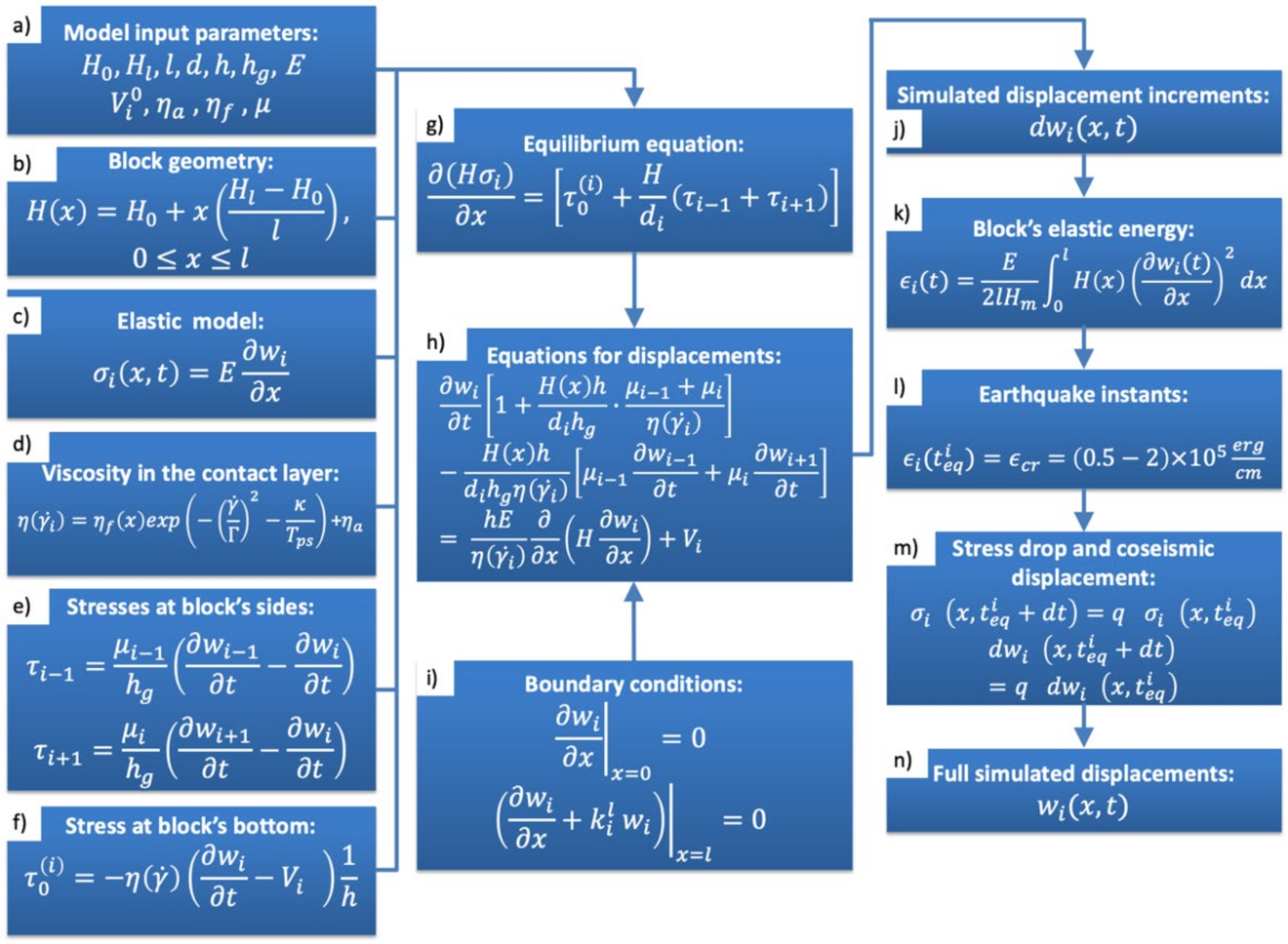
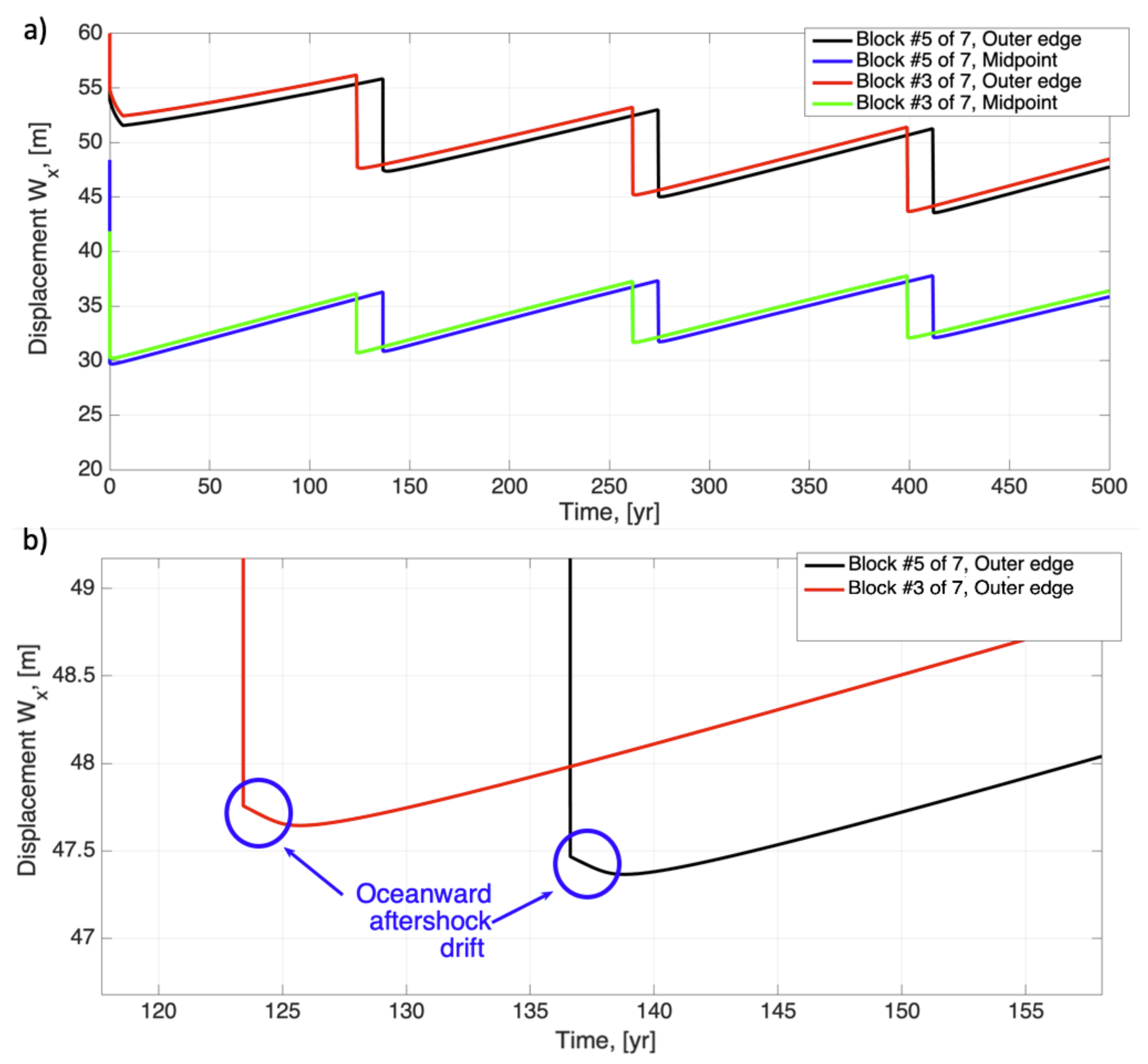
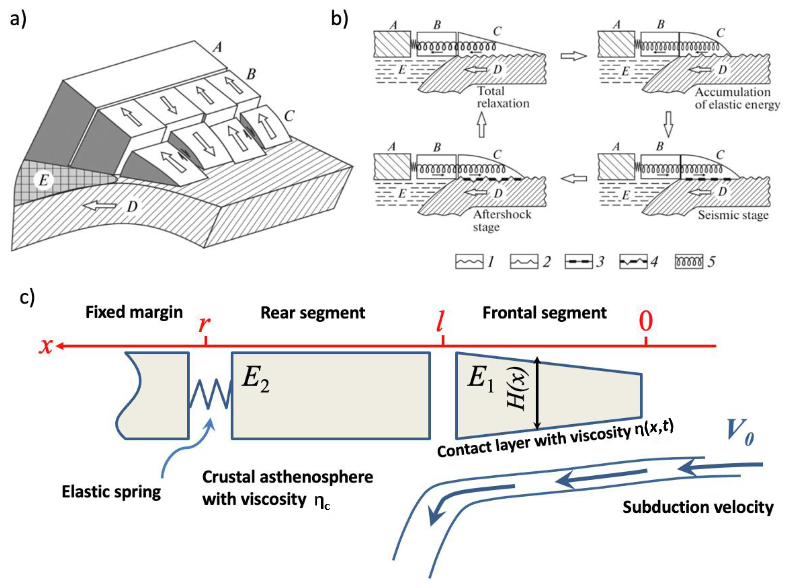
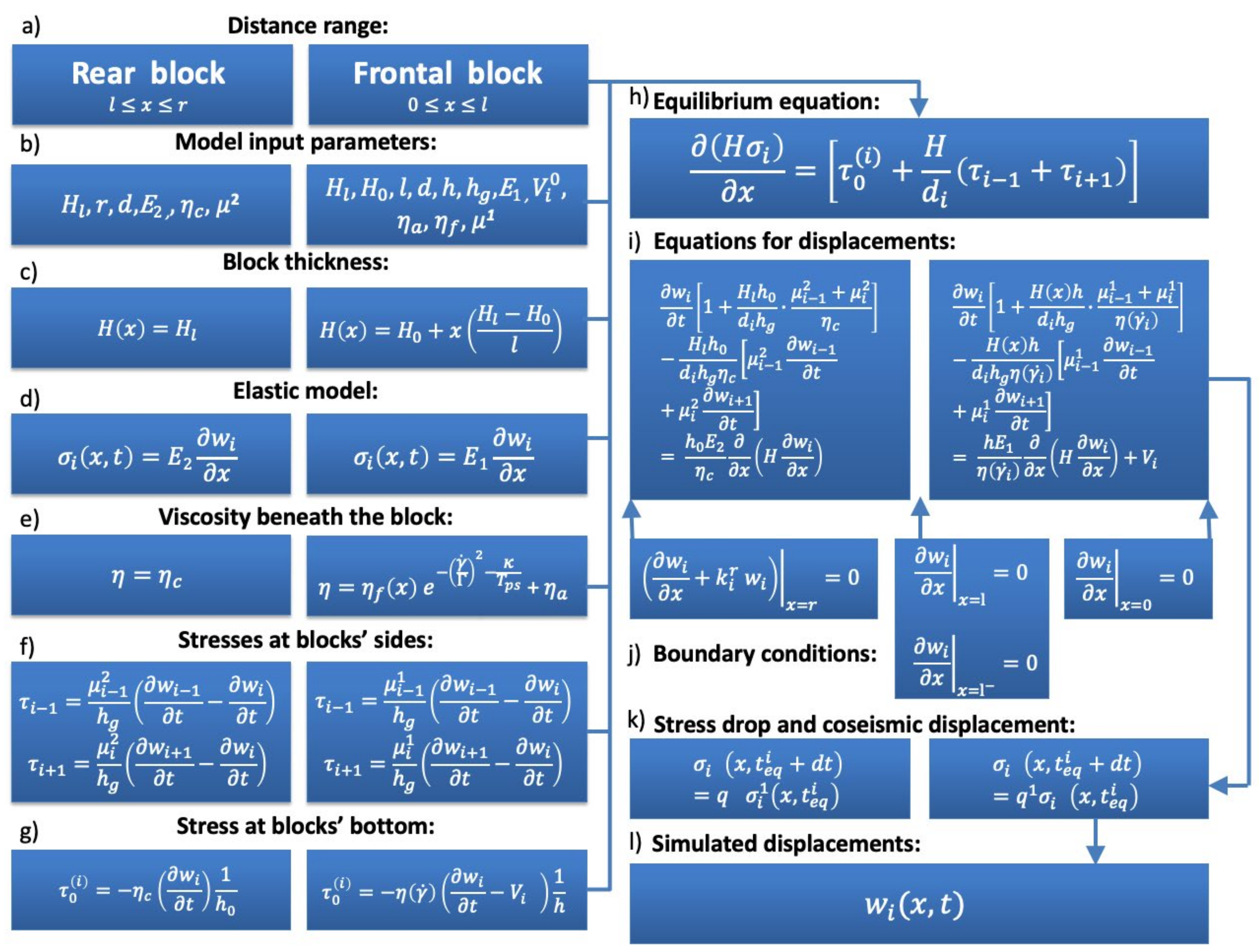
2.1. Keyboard Model of Seismic Cycles of Great Subduction-Associated Earthquakes

The keyboard model was originally proposed in a series of papers by L. Lobkovsky and his colleagues [20]. Here, we briefly cover this concept both in aspects of geometrical structure and numerical formalism allowing for the simulation of stresses and displacements over the system’s evolution cycle.

Geometrically, the modeled region consists of a series of elastic blocks forming a keyboard-like structure aligned with the subduction trench (Figure 1a). Each block is sitting on top of subducting lithosphere, which is constantly moving underneath the continent with velocity V, and there is a thin viscous contact layer separating the block and subducting plate. Tangential stresses acting at the blocks’ bottom due to subduction cause the blocks to move slowly away from the trench (continent-ward motion), leading to build up of the elastic stress within each block until the critical stress value is reached and blocks instantly jump towards the ocean. Thus, the evolution of the system follows a certain periodic pattern (Figure 1b), with repeated phases of stress accumulation, instantaneous stress release (earthquake), and postseismic relaxation.

Transition from the stress accumulation to stress release, followed by aftershock relaxation, occurs once any of the frontal blocks reaches a certain critical energy. To ensure the model’s capability of predicting nonlinear kinematic behavior during the cycle, the contact layer viscosity is assumed variable, taking higher or lower values depending on the strain rate. The numerical scheme applied for simulating the cyclic dynamics, is described by a system of equilibrium equations connecting stresses in the given block and all the neighboring blocks, expressed in terms of the displacement velocities. These essentially depend on viscosities of the contact layer material and the crustal asthenosphere beneath the rear block, as well as viscosity of destructed zones separating blocks laterally.

In describing the model’s mathematical formalism, we will follow notations used in the original paper [20], and present the entire calculation scheme as a flowchart in Figure 2. Model inputs (Figure 2a) include series of parameters defining both geometry and mechanical properties (rheology) of the structure to produce the spatial and temporal distributions of horizontal displacement $w_i\left(x,t\right)$ for any given (ith) block ($i=2, 3,\dots ,m-1)$. The block geometry is given by its lateral dimensions l and d (along x- and y-directions, respectively), and thickness $H\left(x\right)$, which varies from $H_0$ at the outer side of the block to $H_l$ at its inner side (Figure 2b). Typically, $l$ is between 100 to 300 km, while d is 30 to 200 km, depending on a specific structure in a particular subduction zone (

Table 1. Main characteristics of the structure and seismic cycle in Kuril-Kamchatka, Japan, and Chile subduction zones, according to our studies and available data.

Subduction Zone	Block Width/Length, km	Block Length (Frontal/Rear Segment), km	Cycle Period, yrs	Horizontal Coseismic/Aftershock Displacement at Rear Segment, cm
Kuril-Kamchatka	30–100 [15]	100/100 [15]	140 ± 60 [23]	50/50 [19]
Japan	100–150 [24,25]	200/300 [24,25]	100–1000 [21,26]	50–200/10–50 [18]
Chile	100–200 [27,28,29,30]	100/300 [27,28,29,30]	63–176 [31]	5–50/50–80 [17]

).

Mechanically, the mean compressional stress in x-direction is proportional to x-component of deformation (Figure 2c), with $E$ being the elastic modulus of the block. The block is also experiencing tangential stresses ${\tau }_{i-1}$ and ${\tau }_{i+1}$ arising due to the friction of the blocks’ lateral boundaries with neighboring blocks (Figure 2e) as well as the stress ${\tau }_0^{\left(i\right)}$ acting on the bottom surface due to the viscous contact layer, Figure 2f. The latter depends on the strain rate in the contact layer with thickness $h$, written as $\dot{\gamma }=\left(\frac{\partial w_i}{\partial t}-V_i^{}\right)\frac{1}{h}$ ($V_i^{}$ is subduction rate beneath the block), and effective viscosity of the contact layer $\eta \left(\dot{\gamma }, x,t\right)$ (Figure 2d). The viscosity $\eta \left(\dot{\gamma },x,t\right)$ is described by a monotonic function of the strain rate, reflecting the transition from the stationary viscosity ${\eta }_f^{}$ describing the rheology of the contact layer during the interseismic phase of the cycle to a lower postseismic phase viscosity ${\eta }_a^{}$, associated with the contact layer destruction caused by the recently-occurred earthquake. Here $\mathsf{\Gamma }$ denotes the viscosity recovery parameter ($\mathsf{\Gamma }$ = 10⁻⁴ $\frac{1}{yr})$, $\kappa$ = 0.2–0.5 yr is characteristic time required for the contact layer defects to be healed, and $T_{ps}$ is the time passed since the last earthquake in a given block.

The lateral side stresses (Figure 2e) depend on the thickness of the viscous material filling the interblock faults $h_g$, as well as ${\mu }_{i-1}^{}$ and ${\mu }_i^{}$, viscosities of that material between neighboring blocks number. The stress-strain state is assumed to satisfy the stress equilibrium equation (Figure 2g), where $d_i$ is the block size along strike direction, parallel to the trench line.

Table 2. Typical values for parameters of viscous elements of the model according to [20].

Contact Layer Thickness, $\mathit{h}$	Stationary Viscosity of the Contact Layer, ${\mathit{\eta }}_{\mathit{f}}^{}$	Postseismic Viscosity of the Contact Layer, ${\mathit{\eta }}_{\mathit{a}}^{}$	Interblock Fault Thickness, ${\mathit{h}}_{\mathit{g}}$	Interblock Viscosity, $\mathit{\mu }$
~0.5 km	~1019 Pa·s	~1018 Pa·s	~1 km	~4 × 1018 Pa·s

shows typical values of the above parameters following [20].

Substitution of expressions for stresses into equilibrium equation yields the series of equations in terms of displacement w (Figure 2h). Additionally, the boundary conditions are applied (Figure 2i), which have the meaning that the outer edges of the frontal blocks are free, while the rear edges undergo elastic interaction with the fixed margin controlled by the rigidity coefficient $k_i^r$.

The above mathematical formalism is characterized by significant nonlinearity. To solve the problem, we apply an explicit finite-difference method yielding displacement increments $\Delta W_{i, j}^k$ at nodal points $x_i,y_j$ within each block updated at time instants $t_k$ (Figure 2j). Evolution of the block system is controlled by the conditions for dumping the accumulated elastic energy in the form of an abrupt decrease in compressional stresses at time instants $t_{eq}^i$, corresponding to earthquakes, occurring when the block reaches the threshold energy ${ϵ}_{cr}$ (Figure 2k–n). Note that this condition is equivalent to an instantaneous change in displacement. Specific time instants of the earthquakes, $t_{eq}^i$, are determined from the equality of accumulated energy to the threshold value (critical energy) ${ϵ}_{cr}$(Figure 2l) prespecified according to available estimates within range $\left(0.5-2\right)\times {10}^5\frac{erg}{cm}$ [20] ($H_m=\left(H_0+H_l\right)/2$ is the mean thickness of the block).

Obviously, to start the iterative procedure of the solution, one needs the initial displacements to be specified at zeroth step for each point/block. Although not known in practice, since we are lacking historical geodetic data, these might be calculated from random stresses, chosen within the range of 100 to 300 Bar.

Over time, the system shows the tendency to stabilize and follow a specific cyclic pattern, no matter what specific initial stresses/displacements had been used at the starting point. The choice of initial values only affects the time instants at which the blocks reach critical energy, while other properties of the cycle (i.e., cycle period and the shape of kinematic parameters variation over time) remain constant.

The simulated motion patterns computed for a series of typical parameters mentioned above show a sufficient agreement with observational data in terms of cycle duration (around 150–250 years, Figure 3a) and contain characteristic features, with aftershock oceanward motion of the blocks being the most pronounced one (Figure 3b). Below we discuss its possible geomechanical explanations in the light of the up-to-date GNSS observational data.

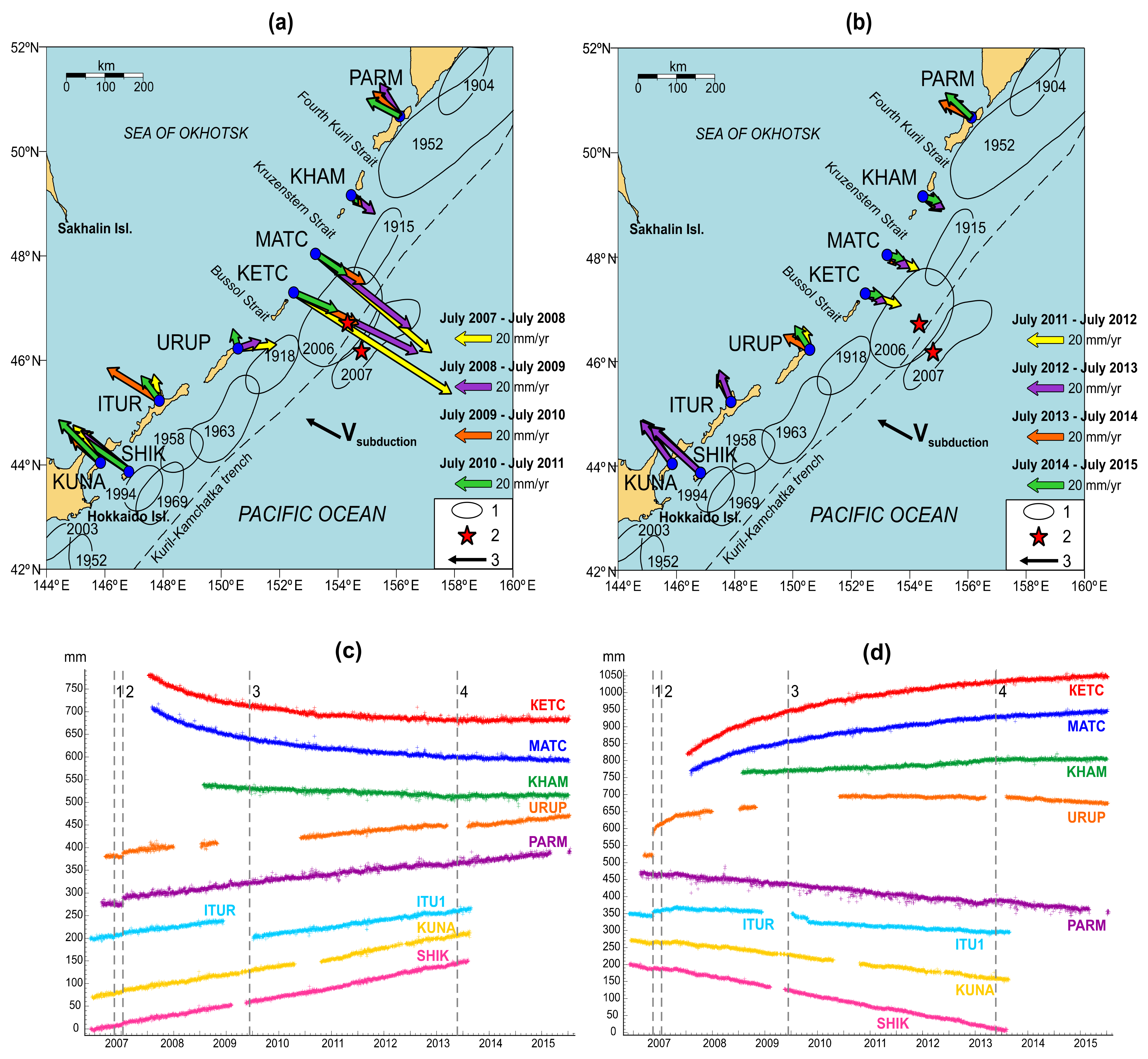
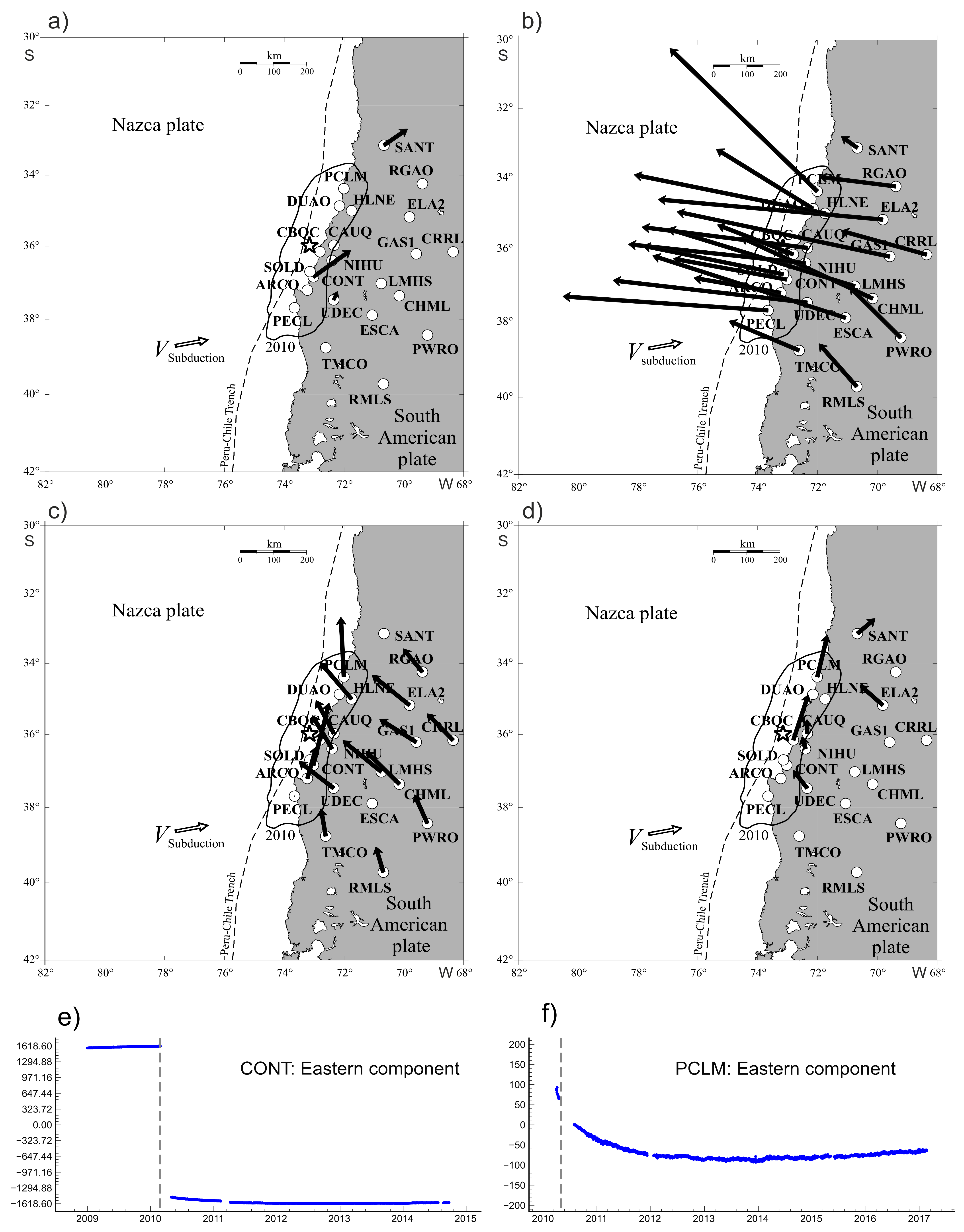
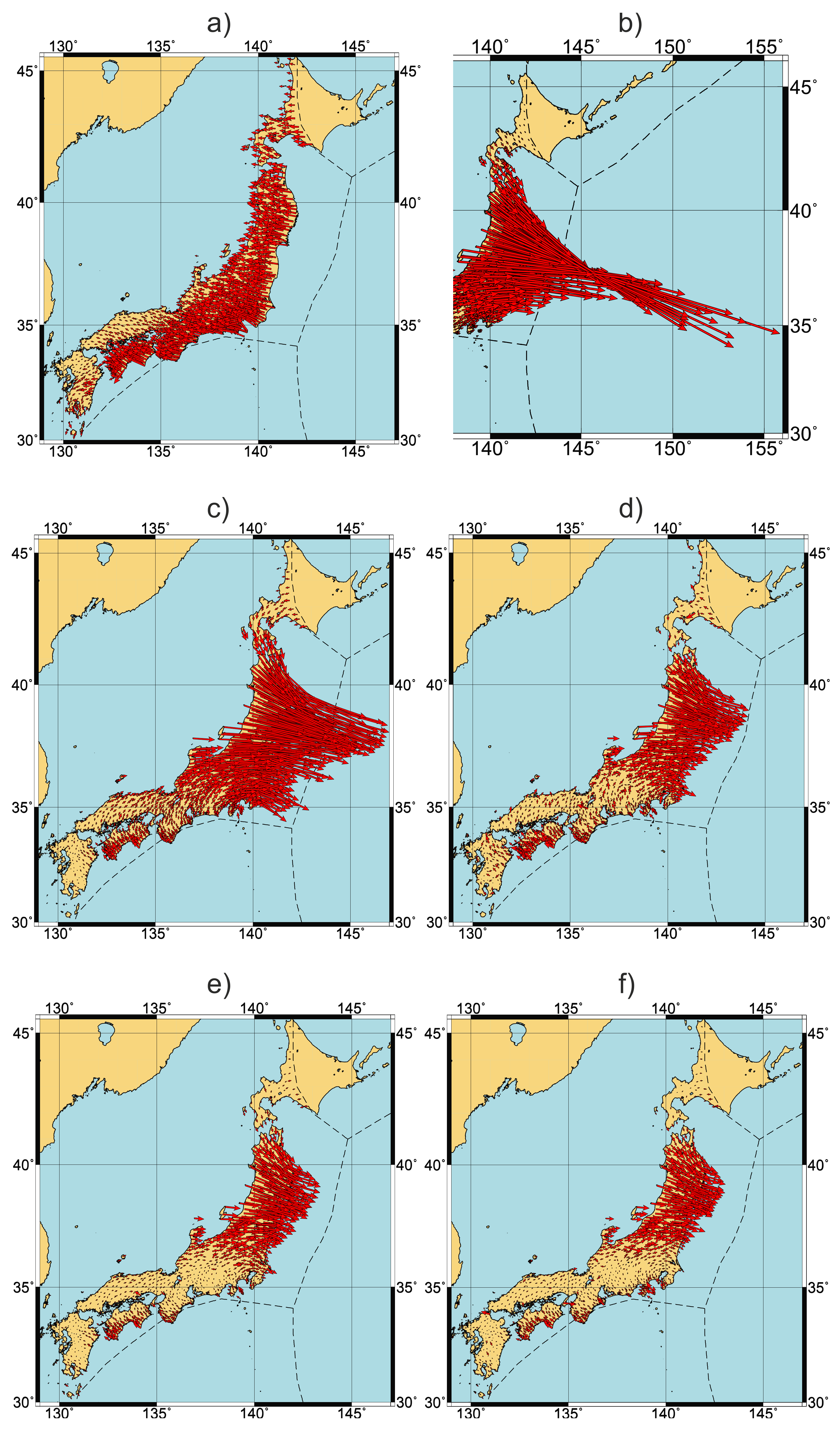
2.2. GNSS-Measured Motions and Stress-Deformation Cycle in Subduction Regions

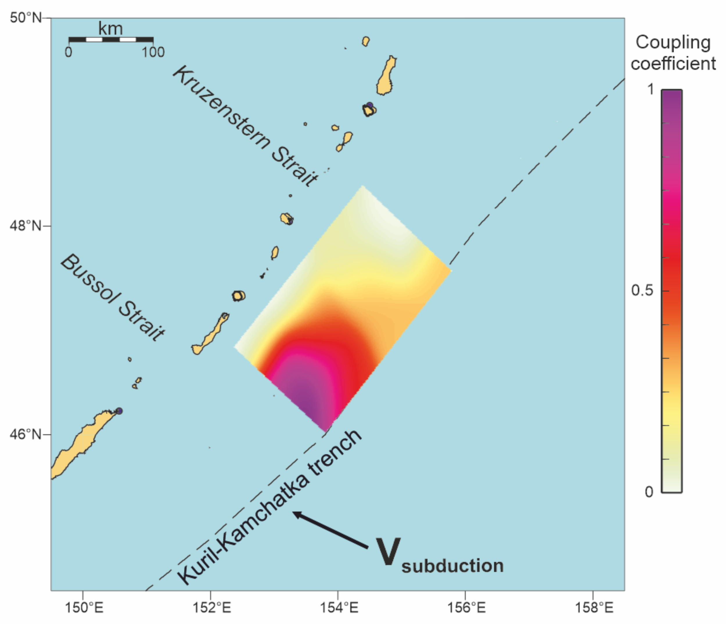
Understanding stress-deformation cycle (SDC) [32] mechanisms in subduction zones is critically important for the long-term large earthquake prediction and seismic hazard assessment [19]. Over decades, a number of concepts have been proposed to explain the SDC features, with the so-called asperity model being the most promoted one [12]. We believe that it is crucial that those models be validated by comparing the predicted behavior with the observed motion data, which has become possible since the high-precision GNSS-based geodetic observations had been launched. GNSS stations deployed in active regions including subduction zones, had made the long-term displacement and velocity data series available, which totally changed the landscape in tectonics and seismology studies.

In a series of previous studies, we analyzed GNSS-measured motions in the Kuril subduction zone following the 2006–2007 Simushir earthquakes [16] (Figure 4), Chile subduction zone following the 2010 Maule earthquake [17] (Figure 5), and Japan subduction zone following the 2011 Tohoku earthquake [18] (Figure 6 and Figure 7), with primary attention paid to horizontal displacements.

Main features of the observed Earth’s surface motions include a slow background continent-ward motion (Figure 5a and Figure 6a), which lasts up to 75% of the duration of the seismic cycle [32] and then is suddenly interrupted by an abrupt oceanward dislocation in source-neighboring areas at the instance of the seismic event (Figure 6b), followed by the continuous motion of the continent-side lithosphere in source-neighboring areas towards the oceanic plate. These postseismic oceanward displacements are unsteady in time and along the strike of the trench. The Figure 4a,b, Figure 5c,d and Figure 6c–f show annual variations of Earth’s surface postseismic motions in the vicinity of source regions of 2006 Simushir, 2010 Maule, and 2011 Tohoku earthquakes, respectively. Despite the fact that each of the regions under consideration has a different tectonic structure and the spatial density of our data varies greatly, we observe similar patterns of postseismic motions: (a) postseismic drift occurs in the direction towards the ocean, and (b) different portions of lithosphere may experience motion in opposite directions at the same time. Such abrupt changes in the direction of motions of adjacent areas of the Earth’s surface in the framework of models assuming a continuous medium will cause large deformations between them. This behavior is seen for all three events in consideration and implies the existence of geomechanical process responsible for the above motions. Obviously, the well-known asperity model lacks the ability to explain the post-quake oceanward drift, occurring in particular regions, while the neighboring territories may move in the opposite (normal) direction. At the same time, the proposed keyboard model can provide natural explanation for observed motions during preseismic, coseismic, and postseismic stages of the seismic cycle. The slow background continent-ward motion (Figure 5a and Figure 6a) is associated with stationary elastic compression of frontal and rear blocks during the interseismic stage. These blocks at the instance of the seismic event are abruptly shifted towards the ocean, which triggers the observed continued oceanward motions of the Earth’s surface. The almost independent displacements of seismogenic blocks also explain the opposite directions of Earth’s surface motions along the oceanic trench during the postseismic stage of the seismic cycle (Figure 4a,b, Figure 5c,d and Figure 6c–f). The observed difference in postseismic motions in the direction perpendicular to the trench (Figure 5c,d) is due to the presence of viscous friction at the bottom of the rear blocks and the presence of a viscous response in the asthenospheric wedge to a coseismic stress drop [19].

3. Results

The motion patterns discussed above provide strong GNSS data-based evidence for alternation of prevalent motion direction over the cycle. At the same time, available geological and seismological data suggest the existence of the fault interfaces separating the offshore frontal blocks from the onshore rear ones [15,33,34], which means that the complete geomechanical model should incorporate both frontal and rear structural parts, allowing for a complex interaction between them. The above considerations indicate the need for modification of the original model [20] in order to take into account the discontinuities both in the frontal and rear parts of the island arc.

In terms of geometry, the two-segment keyboard-block model is represented by a series of elastic blocks forming two chains separated by fault zones extending along the subduction axis (Figure 8). In most cases, the model allows for a relatively simple quasi one-dimensional approximation, limiting the analysis to a single strain component perpendicular to the strike (subduction axis), describing the motion of blocks relative to the subducted lithospheric plate. The submerging plate is separated from the overhanging block by a relatively thin contact layer characterized by nonlinear viscous rheology, with its viscosity essentially depending on the rate of relative motion of the block’s bottom and the subducted plate surface. Nonlinear behavior implies an increase in viscosity when the strain rate is low and block is moving towards the continent (stress accumulation phase), followed by abrupt decrease during the coseismic stage due to the destruction of the material of this layer at the instant of the earthquake, which contributes to the reverse sliding of the block towards the trench in the process of partial release of accumulated elastic stress during the aftershock stage. The transition from the stress accumulation stage to coseismic stage is controlled by an abrupt change (release) of stresses at the instant of an earthquake upon reaching a certain critical stress value (Figure 8b).

Modification of the model’s mathematical formalism involves introducing two separate model domains (corresponding to each of two blocks), and applying appropriate equations within each of them (see Figure 9). An important difference from the original model is that mechanical properties, strain rate and viscosity beneath the blocks are defined in a different way for each block.

The frontal (outer) segment falls within x-coordinate range $0\le x\le l$, while the rear (inner) one lies within $l\le x\le r$. We assume that the gaps between the frontal and rear segments ($x=l)$, as well as between the rear segment and fixed margin ($x=r)$ are negligibly small compared to the block size. Similar to original single-segment model, the computational scheme applied for simulating the cyclic dynamics is described by a system of equilibrium equations connecting stresses in the given frontal-segment (seismogenic) block, rear-segment block, and all the neighboring blocks (Figure 9h).

The boundary conditions applied at the model boundaries (Figure 9j) define the behavior of not only outer edges of the frontal blocks (free moving) and elastic interaction of the rear blocks with the fixed margin, but also of the contact point separating the rear and frontal segments. This condition is variable, depending on the current state of the seismic cycle. During the stress accumulation phase (interseismic stage), the frontal block motion is fully transferred to the rear segment, while during the postseismic (aftershock) phase of the cycle, the segments are considered to be separated by a fluid-filled “gap” due to the possible different rates of backward motion of the frontal and rear blocks towards the ocean following the abrupt stress drop caused by the seismic event. These different rates are due to the viscous friction on the bottom of the rear block which may prevent its elastic straightening. Duration of the postseismic phase is defined by convergence of the segments after the frontal block changes the direction of its motion and starts moving towards the continent, which indicates the transition of the cycle to the stress accumulation phase.

Similar to the original calculation [20], we discretize the problem both in terms of time t with step $\mathsf{\Delta }t$ ($t_k=k·\Delta t$) and $x$ with step $\mathsf{\Delta }x$ ($x_j=j·\Delta x$), so that nodes x_j ($j=1,\dots ,L)$ fall within the frontal block, while those with $j=L+1,\dots ,N$ correspond to the rear block. In discrete formulation, the problem takes form.

For the frontal blocks:

$$\begin{array}{c}\Delta W_{i, j}^k\left[1+\frac{H_{j}h}{d_i{h}_g{\eta }_{i, j}^k}\left({\mu }_{i-1}^1+{\mu }_i^1\right)\right]-\frac{H_{j}h}{d_i{h}_g{\eta }_{i, j}^k}\left({\mu }_{i-1}^1\Delta W_{i-1,j}^k+{\mu }_i^1\mathsf{\Delta }{W}_{i+1,j}^k\right)\\ =\frac{h{E}_1}{{\eta }_{i, j}^k}\frac{\mathsf{\Delta }t}{{\left(\mathsf{\Delta }\mathrm{x}\right)}^2}\left[H_j\left(W_{i, j+1}^k-2W_{i, j}^k+W_{i, j-1}^k\right)+\mathsf{\Delta }x\left(\frac{H_l-H_0}{l}\right)\left(W_{i, j+1}^k-W_{i, j}^k\right)\right]+V_i^1\mathsf{\Delta }t\\ j=2,\dots , L; i=2, \dots , m-1 \end{array}$$

(1)

For the rear blocks:

$$\begin{array}{c}\Delta W_{i, j}^k\left[1+\frac{H_{l}h}{d_i{h}_g{\eta }_{i, j}^k}\left({\mu }_{i-1}^2+{\mu }_i^2\right)\right]-\frac{H_{l}h}{d_i{h}_g{\eta }_{i, j}^k}\left({\mu }_{i-1}^2\Delta W_{i-1,j}^k+{\mu }_i^2\mathsf{\Delta }{W}_{i+1,j}^k\right)\\ =\frac{h{E}_2}{{\eta }_{i, j}^k}\frac{\mathsf{\Delta }t}{{\left(\mathsf{\Delta }x\right)}^2}\left[H_l\left(W_{i, j+1}^k-2W_{i, j}^k+W_{i, j-1}^k\right)\right]\\ j=L+1,\dots , N-1; i=2, \dots , m-1. \end{array}$$

(2)

To ensure the scheme convergence, the time step $\mathsf{\Delta }t$ and x-spacing $\mathsf{\Delta }x$ must be related as $\mathsf{\Delta }t<\frac{{\eta }_{min}{\left(\mathsf{\Delta }x\right)}^2}{2HhE}$, where ${\eta }_{min}$ is the minimum viscosity in the contact layer, and E is elastic modulus of either frontal or rear block.

Boundary conditions are written as:

$$W_{i, 1}^k=W_{i, 2}^k,$$

(3)

$$W_{i, L}^k=\frac{W_{i, L-1}^k}{1+k_i\Delta x},$$

(4)

$$W_{i, L+1}^k=W_{i, L}^k, t_k \mathrm{during} \mathrm{interseismic} \mathrm{phase},$$

(5)

$$W_{i, L+1}^k=W_{i, L+2}^k, t_k \mathrm{during} \mathrm{postseismic} \mathrm{phase}.$$

(6)

Similar to the original single-segment model, the evolution of the block system described by expressions (1–2), (5–6) is controlled by the conditions for dumping the accumulated elastic energy in the form of an abrupt decrease in compressional stresses at $t_{eq}^i$, corresponding to earthquakes, occurring when the frontal block reaches the threshold energy ${ϵ}_{cr}$:

$${\sigma }_i^1\left(x, t_{eq}^i+1\right)=q^1{\sigma }_i^1\left(x, t_{eq}^i\right),$$

(7)

$${\sigma }_i^2\left(x, t_{eq}^i+0\right)=q^2{\sigma }_i^1\left(x, t_{eq}^i-0\right),$$

(8)

Note that this condition is equivalent to an instantaneous change in displacement, with some coefficients that take into account the differences in the elastic modulus between the frontal and rear segments. The specific time instants of the earthquakes, $t_{eq}^i$, are determined from the expression:

$${ϵ}_i\left(t_{eq}^i\right)=\frac{E}{2l{H}_m}{{\displaystyle \int }}_0^{l}H\left(x\right){\left(\frac{\partial w_i\left(t_{eq}^i\right)}{\partial x}\right)}^{2}dx={ϵ}_{cr}$$

(9)

To demonstrate the main features of the model kinematics, we have performed series of simulations, showing the evolution of the model over a 500-year time interval (Figure 10).

An important feature of the model behavior is the existence of oceanward motion of the entire rear segment following every subsequent earthquake (a postseismic or aftershock stage). Modeling of this oceanward motion is of great importance for better assessment of the duration of the seismic cycle and the time moment of the transition of subduction zone to the next seismic cycle. The duration of the aftershock phase depends on the rheological parameters of the medium and can reach up to 50 years in the rear and central part of the rear block and a few years at its frontal edge. Our tests also helped us determine the limits for the viscous parameters of the model. We found that the model behaves in an expected way (accumulation of elastic stress occurs in a reasonable time range (See Table 1)) for the viscosity of the contact layer and the asthenosphere lying in the range of 0.1–1 × 10¹⁹ Pa·s. Lower viscosity (less than 10¹⁸ Pa·s) causes numerical instability of the solution. In the case of higher viscosity (of the order of 10²⁰ Pa·s), the slow (at around 1 cm/year) oceanward motion persists all over the cycle, and the rear block does not experience any continent-ward motion at all. The obtained estimates for model viscous parameters are consistent with the earlier results lying in the range 5 × 10¹⁷–5 × 10¹⁹ Pa·s [35,36,37,38,39,40].

4. Discussion

We believe that employment of the fault-block models seems to be the most promising approach, which allows for more realistic quantitative characterization of the seismic deformation process [19], and propose the generalized two-segment keyboard model [22] as a geomechanical concept capable of explaining the SDC and kinematics in the subduction regions. It is also clear, that validation of such model is only possible through onshore GNSS observations, thus making the problem weakly constrained and unstable, given the lack of data on particular properties of the model.

To verify the above assumptions, we performed a numerical simulation of series of seismic cycles using initial and generalized formulations of keyboard model with stochastic behavior of parameters governing the critical amount of accumulated elastic energy and the amount of relaxed energy. During the simulations the model parameters were constrained to values that are typical for the Kuril subduction system ($E_{1 }$ = 29 GPa, $E_2$= 80 Gpa, $d_i$= 200 km, frontal block length = 100 km, rear block length = 200 km, effective viscosity of the contact layer and the asthenosphere = ${10}^{19}$ Pa·s). We also performed a comparison of the obtained model parameters with ones calculated earlier using the continuum medium model [19] and with geophysical data.

We assumed that the modeled coseismic slip distribution in the source zone of the 2006 Simushir earthquake [19] according to the asperity model [12] represents the preseismic mechanical coupling that was ruptured at the time of the main shock. Such suggestion helps us to construct a model of coupling distribution in the source zone of the 2006 Simushir earthquake (Figure 11). This model allows us to calculate the characteristic time of stress accumulation (i.e., seismic cycle duration) in the source zone of the 2006 Simushir earthquake (

Table 3. Main characteristics of the seismic deformation cycle in the Kuril-Kamchatka subduction zone.

	Geological+ Geophysical Data [32]	Continuous Medium Model [19]	Mechanical Keyboard Model	Generalized Mechanical Keyboard Model
Seismic cycle duration	140$\pm$60 years	159 years	60–267 years (av. 136 years)	40–338 years (av. 162 years)
Postseismic stage duration	Up to 35–50 years	0.5 years (afterslip) up to 10 years (viscoe-lastic relaxation)	2–7 years	1–5 years
Coseismic horizontal surface displacements	─	55 × 10−2 m (GNSS observations)		10 × 10−2–1.8 m (depends on distance from trench and magnitude)

) using known coseismic slip distribution and magnitude and direction of the plate convergence vector [41].

In Table 3 and Figure 12 we present the results of modeling the dynamics of seismogenic blocks in the middle part of the Kuril island arc for 1400 years (10 times the mean duration of SDC for Kuril-Kamchatka subduction zone [32]). To simplify the model, the block sizes are assumed to be the same (100 km × 100 km). According to Global CMT Project data [42], large subduction earthquakes of the Kuril Islands are characterized by a focal length of 120 to 250 km. For example, the spatial dimensions of the source zone of the First Simushir earthquake was estimated on the basis of the aftershock distributions recorded in the first 2 months after the earthquake. This megathrust earthquake was the largest event in the central Kuril Islands since 1915 with the source zone of about 230 km × 150 km. Coseismic motions in the source zone affected three seismogenic blocks with a maximum slip along the contact zone up to 12 m [19].

The rheological parameters of the medium were selected during the further modeling according to the results of the previous studies of the First Simushir earthquake [19].

As a result of the simulation, we estimated the total duration of the seismic cycle, which lay between 113 and 330 years with an average value of 196 years and the duration of the postseismic stage, which corresponds to a range of 11–19 years with an average value of ~15 years. These estimates are in good agreement with the real values of the seismic cycle associated with the 2006 Simushir earthquake, which is 226 years [43] and more than 10 years [19], respectively.

For the case of the used rheological parameters of the medium during the realization of seismic cycles, episodes of simultaneous displacements of two adjacent seismogenic blocks were observed, which confirms the possibility of the formation of extended source zones, such as of the First Simushir earthquake (about 200 km).

Comparing the oceanward motion features observed in the original (Figure 3) and modified (Figure 10) models, it is important to notice that although main features may look similar, including the oceanward drift, in the original model the latter is clearly visible only within the outer (frontal) relatively narrow region of the block. At the same time, the middle and rear parts of the block show no evidence of this oceanward motion. In the modified two-segment model, the oceanward drift is observed both at the outer edges of both the frontal and rear blocks, and that is exactly what is seen in GNSS data.

Figure 13 shows the comparison of characteristic simulated motion for the rear block and GNSS-measured displacements recorded during 2007–2015 at four stations located at the Kuril Islands. It can be seen that the modeled behavior is fairly close to that recorded at KETC station, both in terms of coseismic instantaneous displacement and transient motion observed over 8 years post-earthquake.

The analysis of the two-segment model showed that for the rheological and spatial parameters typical for the Kuril subduction zone, the results of the generalized model are quite close to the results of the original keyboard model and the results of previous studies. At the same time, the generalized model allowed us to compare the model displacements with the GNSS data.

5. Conclusions

Analyzing the simulated energy/stress/displacement/velocity datasets, we focus on characteristic features of the seismic-deformation cycle, presenting with repeated phases both in terms of stress accumulation/release and kinematics. Modeled displacement timeseries exhibit the pronounced cyclic behavior, with a characteristic cycle period of about 160 years, which is consistent with the known patterns of megathrust subduction earthquakes. An essential result proving the model’s relevance is the manifestation of the postseismic (aftershock) phase, when the blocks’ motion reverses its normal continent-ward direction, and a backward motion occurs towards the ocean, as observed from GPS velocity data [16,17,18,19]. In simulated data, this behavior is most clearly seen for the frontal blocks, where the duration of backward-motion phase is about 1–5 years, depending on the location (Figure 11).

Simulated data show the model’s capability to predict the cyclic kinematic patterns, being in good agreement with GPS-measured velocity variations, specifically during the post-quake transient phase (Figure 12).

With the further analysis within the framework of the two-segment keyboard-block model, we expect to obtain the estimates of the relevant geomechanical parameters (material properties) through inverting GPS-measured displacement and velocity timeseries data, acquired over the last decades in subduction regions including Kuril-Kamchatka, Japan, Aleutian, and Chile. The inverse problem solution would also provide crucial data on the transition of the block system between the states of the cycle.

References

1. Shebalin, N.V. Selected Publications. Great Earthquakes; Mining Academy Publishing House: Moscow, Russia, 1997; 542p. (In Russian) [Google Scholar]
2. Keilis-Borok, V. Earthquake Prediction: State-of-the-Art and Emerging Possibilities. Annu. Rev. Earth Planet. Sci. 2002, 30, 1–33. [Google Scholar] [CrossRef] [Green Version]
3. Ruff, L.J. Asperity distributions and large earthquake occurrence in subduction zones. Tectonophysics 1992, 211, 61–83. [Google Scholar] [CrossRef] [Green Version]
4. Kaneko, Y.; Avouac, J.P.; Lapusta, N. Towards inferring earthquake patterns from 513 geodetic observations of interseismic coupling. Nat. Geosci. 2010, 3, 363–369. [Google Scholar] [CrossRef]
5. Rosenau, M.; Horenko, I.; Corbi, F.; Rudolf, M.; Kornhuber, R.; Oncken, O. Synchronization of great subduction megathrust earthquakes: Insights from scale model analysis. J. Geophys. Res. 2019, 124, 3646–3661. [Google Scholar] [CrossRef] [Green Version]
6. Kossobokov, V.G.; Keilis-Borok, V.I.; Smith, S.W. Localization of intermediate-term earthquake prediction. J. Geophys. Res. 1990, 95, 12763–12772. [Google Scholar] [CrossRef]
7. Soloviev, A.A.; Gvishiani, A.D.; Gorshkov, A.I.; Dobrovolsky, M.N.; Novikova, O.V. Recognition of Earthquake-Prone Areas: Methodology and Analysis of the Results. Izv. Phys. Solid Earth 2014, 50, 151–168. [Google Scholar] [CrossRef]
8. Sykes, L.R.; Menke, W. Repeat times of large earthquakes: Implications for earthquake mechanics and long-term prediction. BSSA 2016, 96, 1569–1596. [Google Scholar] [CrossRef]
9. Banna, M.H.A.; Taher, K.A.; Kaiser, M.S.; Mahmud, M.; Rahman, M.S.; Hosen, A.S.M.S.; Cho, G.H. Application of Artificial Intelligence in Predicting Earthquakes: State-of-the-Art and Future Challenges. IEEE Access 2020, 8, 192880–192923. [Google Scholar] [CrossRef]
10. Battaglia, M.; Cervelli, P.F.; Murray, J.R. Modeling crustal deformation near active faults and volcanic centers—A catalog of deformation models. In Techniques and Methods; U.S. Geological Survey: Menlo Park, CA, USA, 2013; Book 13, Chapter B1; 96p. [Google Scholar]
11. Madariaga, R. Seismic Source Theory. In Treatise on Geophysics; Elsevier: Amsterdam, The Netherlands, 2015; pp. 51–71. [Google Scholar]
12. Lay, T.; Kanamori, H. An asperity model of large earthquake sequences. In Earthquake Prediction: An International Review; American Geophysical Union: Washington, DC, USA, 1981; pp. 579–592. [Google Scholar]
13. Senatorski, P. Effect of slip-weakening distance on seismic–aseismic slip patterns. Pure Appl. Geophys. 2019, 176, 3975–3992. [Google Scholar]
14. Lobkovsky, L.I.; Mazova, R.K.; Garagash, I.A.; Kataeva, L.Y.; Nardin, I. To analysis of source mechanism of the 26 December 2004 Indian Ocean tsunami. Russ. J. Earth. Sci. 2006, 8, ES5001. [Google Scholar]
15. Baranov, B.V.; Ivanchenko, A.I.; Dozorova, K.A. The Great 2006 and 2007 Kuril Earthquakes, Forearc Segmentation and Seismic Activity of the Central Kuril Islands Region. Pure Appl. Geophys. 2015, 172, 3509–3535. [Google Scholar] [CrossRef]
16. Lobkovsky, L.I.; Baranov, B.V.; Vladimirova, I.S.; Gabsatarov, V.V.; Steblov, G.M.; Garagash, I.A. Post-seismic motions after the 2006–2007 Simushir earthquakes at different stages of the seismic cycle. Dokl. Earth Sci. 2017, 473, 375–379. [Google Scholar] [CrossRef]
17. Lobkovsky, L.I.; Vladimirova, I.S.; Gabsatarov, Y.V.; Baranov, B.V.; Garagash, I.A.; Steblov, G.M. Seismotectonic deformations associated with the 2010 Maule earthquake at different stages of the seismic cycle according to satellite geodetic observations. Dokl. Earth Sci. 2017, 477, 716–721. [Google Scholar]
18. Lobkovsky, L.I.; Vladimirova, I.S.; Gabsatarov, Y.V.; Steblov, G.M. Seismotectonic Deformations Related to the 2011 Tohoku Earthquake at Different Stages of the Seismic Cycle, Based on Satellite Geodetic Observations. Dokl. Earth Sci. 2018, 481, 1060–1065. [Google Scholar] [CrossRef]
19. Vladimirova, I.S.; Lobkovsky, L.I.; Gabsatarov, Y.V.; Steblov, G.M.; Vasilenko, N.F.; Frolov, D.I.; Prytkov, A.S. Patterns of the Seismic Cycle in the Kuril Island Arc from GPS Observations. Pure Appl. Geophys. 2020, 177, 3599–3617. [Google Scholar]
20. Lobkovsky, L.I.; Kerchman, V.I.; Baranov, B.V.; Pristavakina, E.I. Analysis of seismotectonic processes in subduction zones from the standpoint of a keyboard model of great earthquakes. Tectonophysics 1991, 199, 211–236. [Google Scholar] [CrossRef]
21. Ozawa, S.; Nishimura, T.; Suito, H.; Kobayashi, T.; Tobita, M.; Imakiire, T. Coseismic and postseismic slip of the 2011 magnitude-9 Tohoku-Oki earthquake. Nature 2011, 475, 373–377. [Google Scholar] [CrossRef]
22. Lobkovsky, L.I.; Vladimirova, I.S.; Alekseev, D.A.; Gabsatarov, Y.V. Two-element keyboard model of strongest subduction earthquakes generation. Dokl. Earth Sci. 2021, 496, 72–75. [Google Scholar] [CrossRef]
23. Fedotov, S.A. Regularities of distribution of large earthquakes of Kamchatka, Kuril Islands and North-Eastern Japan. Tr. Inst. Fiz. Zemli Akad. Nauk SSSR 1965, 36, 66–93. (In Russian) [Google Scholar]
24. Loveless, J.P.; Brendan, J.M. Geodetic imaging of plate motions, slip rates, and partitioning of deformation in Japan. J. Geophys. Res. 2010, 115, 1–35. [Google Scholar] [CrossRef]
25. Panayotopoulos, Y.; Hirata, N.; Sato, H.; Kato, A.; Imanishi, K.; Kuwahara, Y.; Cho, I.; Takeda, T.; Asano, Y. Investigating the role of the Itoigawa-Shizuoka tectonic line towards the evolution of the Northern Fossa Magnarift basin. Tectonophysics 2014, 615–616, 12–26. [Google Scholar] [CrossRef] [Green Version]
26. Minoura, K.; Imamura, F.; Sugawara, D.; Kono, Y.; Iwashita, T. The 869 Jogan tsunami deposit and recurrence interval of large-scale tsunami on the Pacific coast of northeast Japan. J. Nat. Disaster Sci. 2001, 23, 83–88. [Google Scholar]
27. Melnick, D.; Echtler, H.P. Morphotectonic and geologic digital map compilations of the south-central Andes (36°–42° S). In The Andes—Active Subduction Orogeny; Frontiers in Earth Science; Oncken, O., Chong, G., Franz, G., Giese, P., Götze, H.-J., Ramos, V.A., Strecker, M., Wigger, P., Eds.; Springer: Berlin/Heidelberg, Germany; New York, NY, USA, 2006; Volume 1, pp. 565–568. [Google Scholar]
28. Geersen, J.; Behrmann, J.H.; Völker, D.; Krastel, S.; Ranero, C.R.; Diaz-Naveas, J.; Weinrebe, W. Active tectonics of the South Chilean marine fore arc (35° S–40° S). Tectonics 2011, 30, 1–16. [Google Scholar] [CrossRef] [Green Version]
29. Moreno, M.; Melnick, D.; Rosenau, M.; Baez, J.; Klotz, J.; Oncken, O.; Tassara, A.; Chen, J.; Bataille, K.; Bevis, M.; et al. Toward understanding tectonic control on the Mw 8.8 2010 Maule Chile earthquake. Earth Planet. Sci. Lett. 2012, 321–322, 152–165. [Google Scholar] [CrossRef]
30. Jara-Muñoz, J.; Melnick, D.; Brill, D.; Strecker, M.R. Segmentation of the 2010 Maule Chile earthquake rupture from a joint analysis of uplifted marine terraces and seismic-cycle deformation patterns. Quat. Sci. Rev. 2015, 113, 171–192. [Google Scholar] [CrossRef]
31. Metois, M.; Vigny, C.; Socquet, A. Interseismic Coupling, Megathrust Earthquakes and Seismic Swarms Along the Chilean Subduction Zone (38°–18° S). Pure Appl. Geophys. 2016, 173, 1431–1449. [Google Scholar]
32. Fedotov, S.A. The seismic cycle, possibility of the quantitative seismic zoning, and long-term seismic forecasting. In Seismic Zoning in the USSR; Medvedev, S.V., Ed.; Nauka: Moscow, Russia, 1968. (In Russian) [Google Scholar]
33. DeMets, C. Oblique convergence and deformation along the Kuril and Japan trenches. J. Geophys. Res. 1992, 97, 17615–17625. [Google Scholar] [CrossRef]
34. Cross, R.S.; Freymueller, J.T. Evidence for and implications of a Bering plate based on geodetic measurements from the Aleutians and western Alaska. J. Geophys. Res. 2008, 113, B07405. [Google Scholar]
35. Piersanti, A. Postseismic deformation in Chile: Constraints on the asthenospheric viscosity. Geophys. Res. Lett. 1999, 26, 3157–3160. [Google Scholar] [CrossRef]
36. Hu, Y.; Wang, K.; He, J.; Klotz, J.; Khazaradze, G. Three-dimensional viscoelastic finite element model for post-seismic deformation of the great 1960 Chile earthquake. J. Geophys. Res. 2004, 109, B12403. [Google Scholar] [CrossRef]
37. Wang, K. Elastic and viscoelastic models of crustal deformation in subduction zone cycles. In The Seismogenic Zone of Subduction Thrust Faults; Dixon, T.H., Moore, J.C., Eds.; Columbia University Press: New York, NY, 2007; pp. 540–577. [Google Scholar]
38. Bürgmann, R.; Dresen, G. Rheology of the Lower Crust and Upper Mantle: Evidence from Rock Mechanics, Geodesy and Field Observations. Annu. Rev. Earth Planet. Sci. 2008, 36, 531–567. [Google Scholar] [CrossRef] [Green Version]
39. Suito, H.; Freymueller, J.T. A viscoelastic and afterslip postseismic deformation model for the 1964 Alaska earthquake. J. Geophys. Res. 2009, 114, B11404. [Google Scholar] [CrossRef] [Green Version]
40. Sato, T.; Larsen, C.F.; Miura, S.; Ohta, Y.; Fujimoto, H.; Sun, W.; Motyka, R.J.; Freymuller, J.T. Reevaluation of the viscosity of upper mantle beneath southeast Alaska. Tectonophysics 2011, 511, 79–88. [Google Scholar] [CrossRef]
41. Kogan, M.G.; Steblov, G.M. Current global plate kinematics from GPS (1995–2007) with the plate-consistent reference frame. J. Geophys. Res. 2008, 113, B04416. [Google Scholar] [CrossRef]
42. Ekström, G.; Nettles, M.; Dziewonski, A.M. The global CMT project 2004–2010: Centroid-moment tensors for 13,017 earthquakes. Phys. Earth Planet. Inter. 2012, 200–201, 1–9. [Google Scholar] [CrossRef]
43. Rogozhin, E.A. Application of tectonophysical approaches to the solution of seismotectonic problems by the example of the Simushir earthquakes of November 15, 2006 and January 13, 2007 in Central Kuriles. Izv. Phys. Solid Earth 2013, 49, 643–652. [Google Scholar] [CrossRef]
Figure 1. (a) Keyboard model geometry; (b) seismic deformation cycle phases. A is the fixed undeformable continental margin; B is the seismogenic block; C is the block-margin interface; D is the subducting plate; (1) 2-D geometry for the no deformation state; (2) stress accumulation (preseismic) phase; (3) coseismic phase (destruction of the mechanical coupling in the contact layer); (4) postseismic (aftershock) phase with continued oceanward motion of the blocks; (5) spring imitating the elastic interaction between blocks and margin.
Applsci 11 09350 g001
Figure 2. Flowchart showing calculation scheme of the original keyboard model. (a) Model input parameters; (b) block thickness; (c) 1-D elastic model; (d) time-dependent viscosity of the contact layer; (e) stresses acting on lateral sides of the block; (f) stress acting at the block’s bottom; (g) stress equilibrium equation; (h) equation governing displacement evolution; (i) boundary conditions applied at the frontal (x = 0) and rear (x = l) edges of the block; (j) calculating incremental displacements; (k) converting displacements into elastic energy accumulated by the block; (l) condition to identify the instant of the earthquake; (m) stress dumping conditions; (n) output dataset.
Applsci 11 09350 g002
Figure 3. Displacement variations W(x,t), simulated with an original single-segment model for an outer edge and midpoint of blocks. Panel (a) shows an overall cycle pattern for 2 different blocks (assuming 7-block structure), while panel (b) provides a detailed picture showing the postseismic oceanward motion, observed at the outer region of the block.
Applsci 11 09350 g003
Figure 4. GNSS-observed motions in Kuril subduction zone after large Simushir earthquakes modified from [16]. Upper panel shows velocity vectors measured by the Kuril GNSS stations during time intervals from May 2007 to May 2011 (a) and from May 2011 to May 2015 (b). (1) Sources of strongest earthquakes with M ≥ 8; (2) main shocks of earthquakes in 2006 and 2007; (3) subduction velocity equal to 80 mm/yr. The velocities indicated here are relative to the North American lithospheric plate. Lower panel shows northern (c) and eastern (d) components of the displacements of the Kuril network observation points. Dashed vertical lines denote the moments: (1) Simushir earthquake in 2006; (2) Simushir earthquake in 2007; (3) Eruption of Sarychev peak in 2009; (4) deep earthquake of the Sea of Okhotsk in 2013.
Applsci 11 09350 g004
Figure 5. GNSS-observed motions in Chile subduction zone before (a) and after (b,d) large 2010 Maule earthquake modified from [17]. Map plots show the velocity vectors estimated from the Chilean and Argentinean regional satellite geodesy networks data for the time intervals of 27 February 2009–26 February 2010 (a); 28 February 2010–27 February 2011 (b); 28 February 2013–27 February 2014 (c); and 28 February 2016–27 February 2017 (d). Lower panel shows eastward displacement timeseries measured at CONT (e) and PCLM (f) GNSS stations. Displacements are relative to the South American lithospheric plate.
Applsci 11 09350 g005
Figure 6. Surface motions in Japan before (a), during (b) and after (cf) 2011 Tohoku earthquake estimated from GEONET GNSS data, modified from [18]. Red arrows show velocity distributions for time intervals as following: 11 March 2010–10 March 2011 (a); 11 March 2011 (b); 12 March 2011–10 March 2012 (c); 11 March 2012–10 March 2013 (d); 11 March 2013–10 March 2014 (e), and 11 March 2014–10 March 2015 (f). Velocities are relative to the South American lithospheric plate.
Applsci 11 09350 g006
Figure 7. Timeseries for the northern (a) and eastern (b) displacement components recorded at GEONET GNSS station 0033. Dashed vertical line indicates 2011 Tohoku earthquake.
Applsci 11 09350 g007
Figure 8. (a) Three-dimensional geometry of the two-segment keyboard-block model, (b) seismic deformation cycle phases, and (c) vertical plane section for the particular block along x-direction. A is the fixed undeformable continental margin; B is the rear-segment block; C is the frontal-segment block; D is the subducting plate; E is the crustal asthenosphere. (1) Two-dimensional geometry for the no deformation state; (2) stress accumulation (preseismic) phase; (3) coseismic phase (destruction of the crust); (4) postseismic (aftershock) phase with continued oceanward motion of the blocks.
Applsci 11 09350 g008
Figure 9. Flowchart showing calculation scheme of the generalized (two-element) keyboard model. (a) Schematic representation of rear (left) and frontal (right) modeling domains (blocks); (b) model input parameters for the rear (left) and frontal (right) blocks; (c) block thickness; (d) 1-D elastic model; (e) viscosity as function of x and t: constant viscosity beneath the rear block (left), time-dependent viscosity of the contact layer beneath the frontal block (right); (f) stresses acting on lateral sides of the blocks; (g) stress acting at the blocks’ bottom; (h) stress equilibrium equation; (i) equation governing displacement evolution; (j) boundary conditions applied at the frontal edge of the frontal block (x = 0), contact between the frontal and rear blocks (x = l), and rear (x = r) edge of the rear block; (k) stress dumping conditions; (l) output dataset.
Applsci 11 09350 g009
Figure 10. Displacement variations W(x,t), simulated with a two-segment model for a series of points within the rear-segment blocks (x = 150, 160, 175, and 225 km), calculated for a typical set of model parameters (see Table 1).
Applsci 11 09350 g010
Figure 11. Model of the mechanical coupling distribution in the source zone of the 2006 Simushir earthquake. Black arrow displays magnitude and direction of the plate convergence vector [41].
Applsci 11 09350 g011
Figure 12. Simulation of several seismic deformation cycles in Kuril subduction zone for generalized keyboard model. Left column of images shows the displacements of two boundary and one middle points of frontal block, right column shows the displacements of the same points of rear block. Stochastic condition for amount of relaxed and accumulated elastic energy was applied. Initial large displacement is caused by stabilization of the numerical scheme and is ignored in further analysis.
Applsci 11 09350 g012
Figure 13. East-west displacement timeseries measured by Kuril GNSS network following the 2006–2007 Simushir earthquakes (black curves) and modeled displacement data (light blue line) calculated within the interior part of the rear block using the two-segment model. Positive values correspond to eastward (i.e., oceanward) motion.
Applsci 11 09350 g013