Analytical Solution of Stress in a Transversely Isotropic Floor Rock Mass under Distributed Loading in an Arbitrary Direction

Abstract

Rock masses with a distinct structure may present a transversely isotropic character; thus, the stress state in a transversely isotropic elastic half-plane surface is an important way to assess the behavior of the interaction between the distributed loading and the surroundings. Most previous theoretical analyses have considered a loading direction that is either vertical or horizontal, and the stress distribution that results from the effect of different loading directions remains unclear. In this paper, based on the transversely isotropic elastic half-plane surface theory, a stress solution that is applicable to distributed loading in any direction is proposed to further examine the loading effect. The consistency between the analytical solution and numerical simulations showed the effectiveness of the proposal that was introduced. Then, it was utilized to analyze the stress distribution rule by changing the Poisson’s ratio and Young’s modulus of the model. The effects of the formation dip angle on the stress state are also examined. The stress distribution, depending on the physical property parameters and relative angle, is predicted using an analytical solution, and the mechanisms associated with the transversely isotropic elastic half-plane surface subjected to the loading in any direction are clarified. Additionally, extensive analyses regarding this case study, with respect to the mechanical behavior associated with changes in the stress boundary, is available. Hence, the proposed analytical solution can more realistically account for the loading problem in many engineering practices.

1. Introduction

Along with the development of underground engineering construction, layered rock mass is the most familiar type of rock mass due to the existence of directional structural planes. The failure modes and deformation behaviors of transversely isotropic rocks are very different from those of isotropic rock mass under the uniform loading of an arbitrary angle. Therefore, the influence of the mechanical properties of rock materials, particularly under transverse isotropic conditions, is a notably important problem for describing the deformation and failure characteristics of rock masses.

The issues with respect to transversely isotropic rocks are often encountered in mining engineering. Uniaxial and triaxial cyclic tests were sensitive to being strongly influenced by the inclination of loading with respect to the isotropy planes [1]. The direct tensile strength of the initial bedding plane was quantified through laboratory experiments, and the influence of weak planes on the mechanical behaviors of transversely isotropic rocks under uniaxial compression was studied [2,3]. In addition, the fracture mode and failure strength of the rock samples tested in Brazil were characterized with different foliation-loading angles [4,5], of which the digital image correlation (DIC) method was used to study crack initiation and propagation with various anisotropy angles [6]. The relationship among the tensile strength, specimen size, and loading slice angle of the transversely isotropic rocks was revealed from the perspective of size effect, which together control the failure mechanism of transversely isotropic rocks in the Brazilian test [7,8]. The isotropic materials’ response curve was defective because of the neglect of the orthotropic and transversely isotropic cases, and the classical criteria for isotropic materials were generalized for the case of orthotropy as well as transverse isotropy [9]. These laboratory studies have provided a great deal of insight and many valuable results.

In order to identify the distribution of the stress and strength of rock mass affected by the transversely isotropic laminated layers, a number of physical models have been reported [10,11,12,13]. Moreover, the wave phase velocity [14] and ultrasonic response [15] across the transversely isotropic layers were employed and analyzed, creating an effective constitutive model that was capable of describing the bedding plane elastic-plastic matrix equation [16]. The evolution of the mechanical parameters of bedding planes with the internal variable was determined, including the isotropic plane direction and dip angle [17], and the magnitude of the anisotropic elastic constant [18] and its influence under non-uniform action [19]. The studies revealed that the in situ stress ratio and the orientation of the bedding plane significantly affected the load distribution. Theoretical derivation of the anisotropic damage model was given [20], both in the elastic [21] as well as in the post-failure phases [22]. Hu JT et al. [23] and Vu TM et al. [24] proposed a calculation of p-wave travel time marching in a three-dimensional transversely isotropic medium wave step by step. Anisotropic damage models considering loading were induced [25], continuum damage ([26]) was analyzed, and some suggestions were put forward.

The experiments in the lab and the implementations on the worksite [27] showed that according to the structure in the direction of principal stress test [28], assembling produced a set of devices for carrying out an experiment in parallel and perpendicular to the direction of the bedding, analyzing its influence on tunnel convergence [29], and determining the influence of the stratification plane directivity on the supporting structure [30]. Meanwhile, shale stability depended on the direction between the borehole axis and the stratification at the drilling site [31,32]. The concentrations of stress in the wall of a horizontal well in transversely isotropic shale were quantified [33], and the lateral pressure sensitivity [34,35] was obtained.

More recently, the numerical solution of isotropic multilayer viscoelastic porous rock foundations under vertical circular loading was given [36], the displacement continuity condition [37] and non-Darcy flow [38] characteristics were analyzed, and the mechanical and anisotropic characteristics of the rock mass were developed and adopted to explain this based on Goodman’s stiffness equation [39], the double boundary element method [40], the three-dimensional continuum model [41], and the Thomsen parameters [42]. They came to the conclusion that transversely isotropic bedding planes have significant impacts on the analysis of bedding planes.

The above valuable results obtained were developed based on the assumption that loading occurred in the vertical or horizontal direction. Considering the fact that there was a lack of an efficient method to analyze and evaluate the effect of the loading angle with respect to the horizontal plane applied on structures, based on the previous basic work by the authors, the angle was adopted as the variable to propose a method to support the stress distribution. Therefore, the ground responses to distributed loading, considering the influence of an arbitrary angle, require further analysis. In this paper, based on the equilibrium equation, geometric equation, boundary conditions and physical equation, a new analytical model to estimate the stress is established, where the loading inclination is considered. On this basis, a new model was devised for the arbitrary direction under various schemes, and an evaluation of the efficiency for arbitrary direction was proposed by using numerical simulations. The results were given to manifest the analytical computation, which can be used for the advance predictions of loading action. Thus, this paper proposes a theoretical foundation for the evaluation of stress distribution results under an arbitrary direction and offers valuable insights into both theoretical research and actual engineering applications.

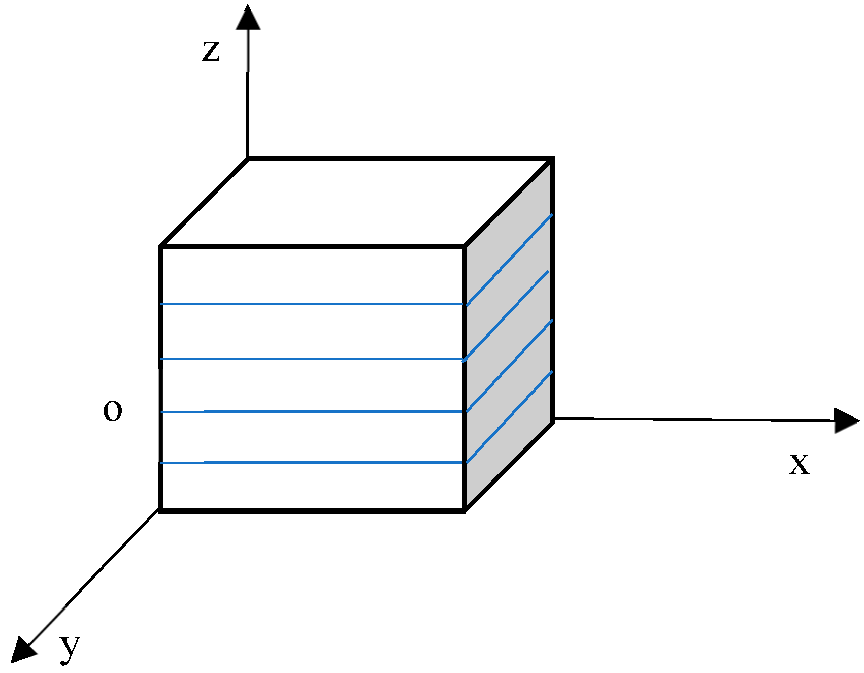
2. The Transverse Isotropic Model of Layered Rock Mass

2.1. The Transverse Isotropic Elastic Constitutive Model

The analytical solution of the distributed loading on the surface of semi-infinite isotropic elastomers has been given, while that of the transversely isotropic floor rocks has not been obtained as layered rock mass is often simplified as a transversely isotropic body in engineering practices, as shown in Figure 1. More specifically, if XOY is a transversely isotropic plane, then the constitutive relation of a transversely isotropic elastomer [43] is:

$$\begin{gathered} \{\begin{array}{c}{\epsilon }_x\\ {\epsilon }_y\\ {\epsilon }_z\\ {\gamma }_{xy}\\ {\gamma }_{yz}\\ {\gamma }_{xz}\end{array}\}=\left[\begin{array}{cccccc}{A}_{11}& A_{12}& A_{13}& 0& 0& 0\\ A_{12}& A_{22}& A_{23}& 0& 0& 0\\ A_{13}& A_{23}& A_{33}& 0& 0& 0\\ 0& 0& 0& A_{44}& 0& 0\\ 0& 0& 0& 0& A_{55}& 0\\ 0& 0& 0& 0& 0& A_{66}\end{array}\right]\left\{\begin{array}{c}{\sigma }_x\\ {\sigma }_y\\ {\sigma }_z\\ {\tau }_{xy}\\ {\tau }_{yz}\\ {\tau }_{xz}\end{array}\right\} \\ \begin{array}{c}{A}_{11}=A_{22}=\frac{1}{E_1},A_{12}=-\frac{{\mu }_1}{E_1},A_{13}=-\frac{{\mu }_2}{E_2}\\ A_{33}=\frac{1}{E_2},A_{44}=\frac{2(1+{\mu }_1)}{E_1},A_{55}=A_{66}=\frac{1}{G_2}\end{array} \end{gathered}$$

(1)

where $E_1$ and $E_2$ are the elastic moduli of the parallel transversely isotropic plane (XOY plane) and the vertical transversely isotropic plane (z-axis direction), respectively; ${\mu }_1$ and ${\mu }_2$ are Poisson’s ratios characterizing the lateral strain response in the plane of transverse isotropy to a stress acting parallel or normal to it, respectively; and $G_2$ is the shear modulus in the vertical isotropic plane.

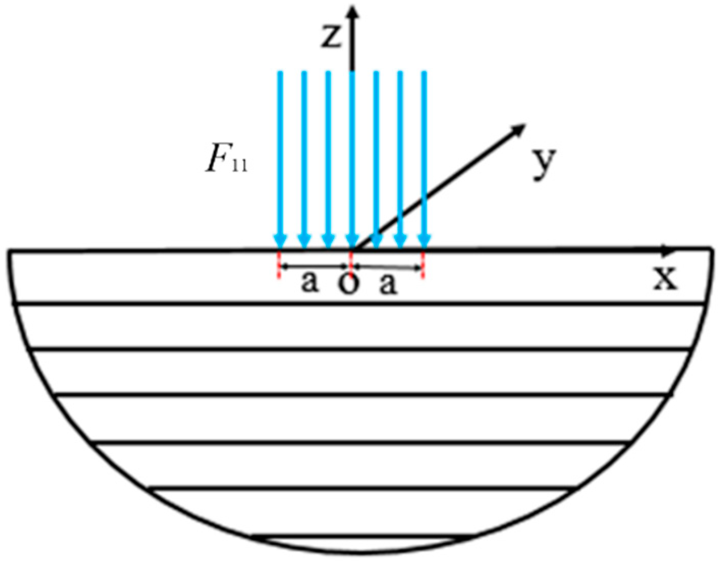
2.2. A Semi-Infinite Plane Subjected to Vertically Distributed Stresses

For the case of the isotropic elastic half-plane subjected to vertical stresses on the point, the coordinate system is established as shown in Figure 2. The XOY plane is assumed to the transverse isotropic plane [44]. If F₁ is the applied stress, the basic equation can be obtained as follows:

(1)

Equilibrium differential equation

$$\{\begin{array}{c}\frac{\partial {\sigma }_x}{\partial x}+\frac{\partial {\tau }_{xz}}{\partial z}+f_x=0\\ \frac{\partial {\sigma }_z}{\partial z}+\frac{\partial {\tau }_{xz}}{\partial x}+f_z=0\end{array}$$

(2)

where $f_x$ and $f_z$ are the volume forces along the X and Z axes, respectively; ${\sigma }_x$ and ${\sigma }_z$ are the normal stresses along the X and Z axes, respectively; and ${\tau }_{xz}$ is the shear stress along the X direction.

(2)

geometric equation

$${\epsilon }_x=\frac{\partial u}{\partial x},{\epsilon }_y=\frac{\partial w}{\partial z},{\gamma }_{yz}=\frac{\partial w}{\partial x}+\frac{\partial u}{\partial z}$$

(3)

where $u$ and $w$ are the displacements along the X and Z axes, respectively.

(3)

physical equations

$$\{\begin{array}{c}{\epsilon }_x=\frac{1}{E_1}\left(1-{\mu }_1{}^2\right){\sigma }_x-\frac{1}{E_2}\left(1+{\mu }_1\right){\mu }_2{\sigma }_z\\ {\epsilon }_z=-\frac{1}{E_2}\left(1+{\mu }_1\right){\mu }_2{\sigma }_x+\frac{1}{E_2}\left(1-\frac{E_1}{E_2}{\mu }_2{}^2\right){\sigma }_z\\ {\gamma }_{xz}=\frac{1}{G_2}{\tau }_{xz}\end{array}$$

(4)

where $E_1$ and ${\mu }_1$ are the elastic modulus and Poisson’s ratio in the transverse isotropic plane; $E_2$ and ${\mu }_2$ are the elastic modulus and Poisson’s ratio in the vertical isotropic plane (z-axis direction); and $G_2$ is the shear modulus in the vertical isotropic plane.

(4)

boundary conditions

When $z=0$, ${\tau }_{xz}=0$, ${\sigma }_z=-p\delta (x)$.

where: $\delta (x)$ is the function of $Dirace$, $\delta (x)=\{\begin{array}{c}\infty ,x=0\\ 0,x\ne 0\end{array}$.

$$\frac{{\partial }^2{\epsilon }_x}{\partial z^2}+\frac{{\partial }^2{\epsilon }_z}{\partial x^2}=\frac{{\partial }^2{\gamma }_{xz}}{\partial x\partial z}$$

(5)

Without considering physical strength, the stress component of the transversely isotropic plane problem is also expressed as:

$${\sigma }_x=\frac{{\partial }^2\phi }{\partial z^2},{\sigma }_z=\frac{{\partial }^2\phi }{\partial x^2},{\tau }_{xz}=-\frac{{\partial }^2\phi }{\partial x\partial z}$$

(6)

where $\phi =\phi (x,z)$ is a $Airy$ function.

The stress function $\phi =\phi (x,z)$ automatically satisfied the equilibrium Equation (2) [45]. The physical Equation (4) is substituted into the deformation coordination Equation (5), and then Equation (6) is deduced to obtain the compatible equation, which is expressed by the stress function as:

$$\frac{1}{E_1}\left(1-u_1^2\right)\frac{{\partial }^4\phi }{\partial z^4}+\left[\frac{1}{G_2}-\frac{2}{E_2}\left(1+u_1\right)u_2\right]\frac{{\partial }^4\phi }{\partial x^2\partial z^2}+\frac{1}{E_2}\left(1-\frac{E_1{u}_2^2}{E_2}\right)\frac{{\partial }^4\phi }{\partial x^4}=0$$

(7)

Note that the solution of the transversely isotropic problem is reduced to seek the stress function satisfying the differential Equation (7) and boundary conditions $\phi =\phi (x,z)$ without regard to physical force. It is very convenient for this differential equation to use the Fourier transform to solve Equation (7). By applying the Fourier transform of Equation (7) to X, it can be obtained as follows:

$$\begin{array}{l}\frac{1}{E_1}\left(1-{\mu }_1^2\right)\frac{d^4\overline{\phi }\left(\xi ,z\right)}{d{z}^4}-{\xi }^2\left[\frac{1}{G_2}-\frac{2}{E_2}\left(1+{\mu }_1\right){\mu }_2\right]\frac{d^2\overline{\phi }\left(\xi ,z\right)}{d{z}^2}\\ +{\xi }^4\frac{1}{E_2}\left(1-\frac{E_1{\mu }_2^2}{E_2}\right)\overline{\phi }\left(\xi ,z\right)=0\end{array}$$

(8)

Equation (8) is a fourth order differential equation with constant coefficients. Considering that the half plane of z < 0, the general solution is:

$$\overline{\phi }\left(\xi ,z\right)=c{e}^{a_1\left|\xi \right|z}+d{e}^{a_2\left|\xi \right|z}$$

(9)

where c and d are the functions of the Fourier transform parameters, which can be determined according to the boundary conditions. a₁ and a₂ are the two positive real numbers of the roots of the quartic algebraic equation with respect to a, whose equations were:

$$\frac{1}{E_1}\left(1-u_1^2\right)a^4+\left[\frac{1}{G_2}-\frac{2}{E_2}\left(1+u_1\right)u_2\right]a^2+\frac{1}{E_2}\left(1-\frac{E_1{u}_2^2}{E_2}\right)=0$$

(10)

By applying the Fourier transform to the boundary conditions in Equation (4), it can be obtained that the boundary conditions in the image domain are:

When $z=0$, ${\tau }_{xz}=0$, ${\sigma }_z=p$.

According to the above analysis results, it can be concluded that:

$${\sigma }_x=\frac{F_1}{\pi }\left[\frac{K_1{A}_1{}^{3}z}{x^2+{(A_{1}z)}^2}-\frac{K_2{A}_2{}^{3}z}{x^2+{(A_{2}z)}^2}\right]$$

(11)

$${\sigma }_{\mathrm{z}}=-\frac{F_1}{\pi }\left[\frac{K_1{A}_{1}z}{x^2+{(A_{1}z)}^2}-\frac{K_2{A}_{2}z}{x^2+{(A_{2}z)}^2}\right]$$

(12)

$${\tau }_{xz}=-\frac{F_1}{\pi }\left[\frac{K_1{A}_{1}x}{x^2+{(A_{1}z)}^2}-\frac{K_2{A}_{2}x}{x^2+{(A_{2}z)}^2}\right]$$

(13)

where

$$\begin{gathered} A_1=\sqrt{\frac{S_{66}/2+S_{12}+\sqrt{{\left(S_{66}/2+S_{12}\right)}^2-S_{11}{S}_{22}}}{S_{11}}} \\ {A}_2=\sqrt{\frac{S_{66}/2+S_{12}-\sqrt{{\left(S_{66}/2+S_{12}\right)}^2-S_{11}{S}_{22}}}{S_{11}}} \\ {S}_{11}=\frac{1-{\mu }^2}{E_1} S_{12}=-\frac{{\mu }_2\left(1+{\mu }_1\right)}{E_2} S_{22}=\left(1-\frac{E_1{\mu }_2{}^2}{E_2}\right)/E_2 S_{66}=\frac{1}{G_2} \\ {K}_1=\frac{A_2}{A_1-A_2} K_2=\frac{A_1}{A_1-A_2} \end{gathered}$$

Based on Equations (11)–(13) and Figure 3, it can be obtained that the distributed stress F₁₁ applied vertically on the transverse isotropic plane and the stress distribution can be expressed as:

$$\Delta {\sigma }_x=\frac{F_{11}}{\pi }\left[\begin{array}{l}{K}_1{A}_1{}^2\left(arc\tan \left(\frac{x+a}{A_{1}z}\right)-arc\tan \left(\frac{x-a}{A_{1}z}\right)\right)-\\ K_2{A}_2{}^2\left(arc\tan \left(\frac{x+a}{A_{2}z}\right)-arc\tan \frac{x-a}{A_{2}z}\right)\end{array}\right]$$

(14)

$$\Delta {\sigma }_z=-\frac{F_{11}}{\pi }\left[\begin{array}{l}{K}_1\left(arc\tan \left(\frac{x+a}{A_{1}z}\right)-arc\tan \left(\frac{x-a}{A_{1}z}\right)\right)-\\ K_2\left(arc\tan \left(\frac{x+a}{A_{2}z}\right)-arc\tan \frac{x-a}{A_{2}z}\right)\end{array}\right]$$

(15)

$${\tau }_{xz}=-\frac{F_{11}}{\pi }\left[\begin{array}{l}{K}_1{A}_1\left[\ln {\left({\left(x+a\right)}^2+{\left(A_{1}z\right)}^2\right)}^{1/2}-\ln {\left({\left(x-a\right)}^2+{\left(A_{1}z\right)}^2\right)}^{1/2}\right]-\\ K_2{A}_2\left[\ln {\left({\left(x+a\right)}^2+{\left(A_{2}z\right)}^2\right)}^{1/2}-\ln {\left({\left(x-a\right)}^2+{\left(A_{2}z\right)}^2\right)}^{1/2}\right]\end{array}\right]$$

(16)

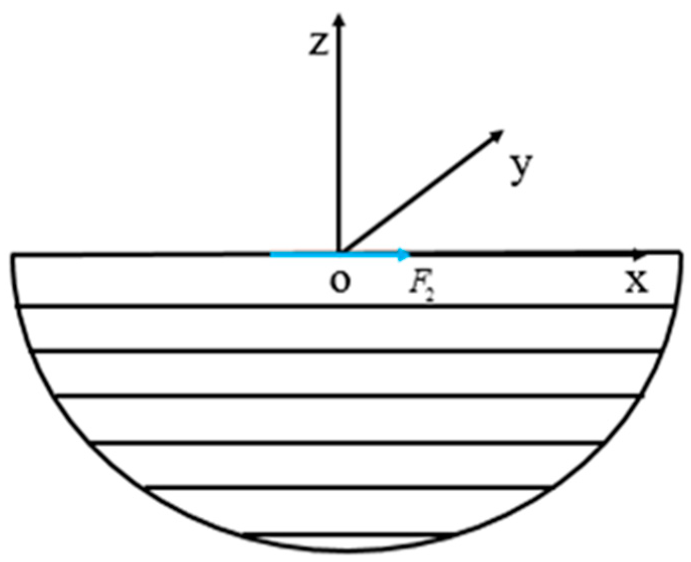
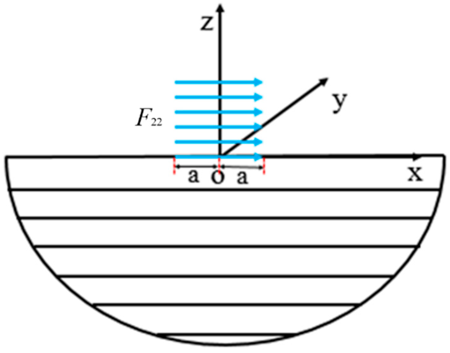
2.3. A Semi-Infinite Plane Subjected to Horizontally Distributed Stresses

There is a semi-infinite body with no physical force, and the concentrated stress F₂ is applied along the plane. The main coordinate is shown as Figure 4.

The solution process of horizontal stress is the same as that of the vertical stress. As such, the stress distribution can be obtained as follows:

$${\sigma }_x=-\frac{F_2}{\pi }\left[\frac{K_1{A}_{1}x}{{(z\tan \alpha )}^2+{(A_{1}z)}^2}-\frac{K_2{A}_{2}x}{{(z\tan \alpha )}^2+{(A_{2}z)}^2}\right]$$

(17)

$${\sigma }_{\mathrm{z}}=-\frac{F_2}{\pi }\left[-\frac{K_1}{A_1}\frac{x}{{(z\tan \alpha )}^2+{(A_{1}z)}^2}+\frac{K_2}{A_2}\frac{x}{{(z\tan \alpha )}^2+{(A_{2}z)}^2}\right]$$

(18)

$${\tau }_{xz}=-\frac{F_2}{\pi }\left[\frac{K_1{A}_{1}z}{{(z\tan \alpha )}^2+{(A_{1}z)}^2}-\frac{K_2{A}_{2}z}{{(z\tan \alpha )}^2+{(A_{2}z)}^2}\right]$$

(19)

If the horizontal stress is uniformly distributed, the coordinate system can be established as shown in Figure 5. Assuming that the width of strip foundation is 2a, and distributed loading F₂₂ is horizontally applied on the transversely isotropic plane, the additional stress at any point in the foundation can be obtained by integrating the above equations in the interval [−a, a], which can be depicted as:

$${\sigma }_x=\frac{F_{22}}{2\pi }\left[K_1{A}_1\cdot \ln \frac{{(x-a)}^2+A_1{}^2{z}^2}{{(x+a)}^2+{(A_{1}z)}^2}-K_2{A}_2\cdot \ln \frac{{(x-a)}^2+A_2{}^2{z}^2}{{(x+a)}^2+{(A_{2}z)}^2}\right]$$

(20)

$${\sigma }_z=-\frac{F_{22}}{2\pi }\left[\frac{K_1}{A_1}\cdot \ln \frac{{(x-a)}^2+A_1{}^2{z}^2}{{(x+a)}^2+{(A_{1}z)}^2}-\frac{K_2}{A_2}\cdot \ln \frac{{(x-a)}^2+A_2{}^2{z}^2}{{(x+a)}^2+{(A_{2}z)}^2}\right]$$

(21)

$${\tau }_{xz}=\frac{F_{22}}{\pi }\left[K_1\left(a\tan \frac{x-a}{A_{1}z}-a\tan \frac{x+a}{A_{1}z}\right)-K_2\left(a\tan \frac{x-a}{A_{2}z}-a\tan \frac{x+a}{A_{2}z}\right)\right]$$

(22)

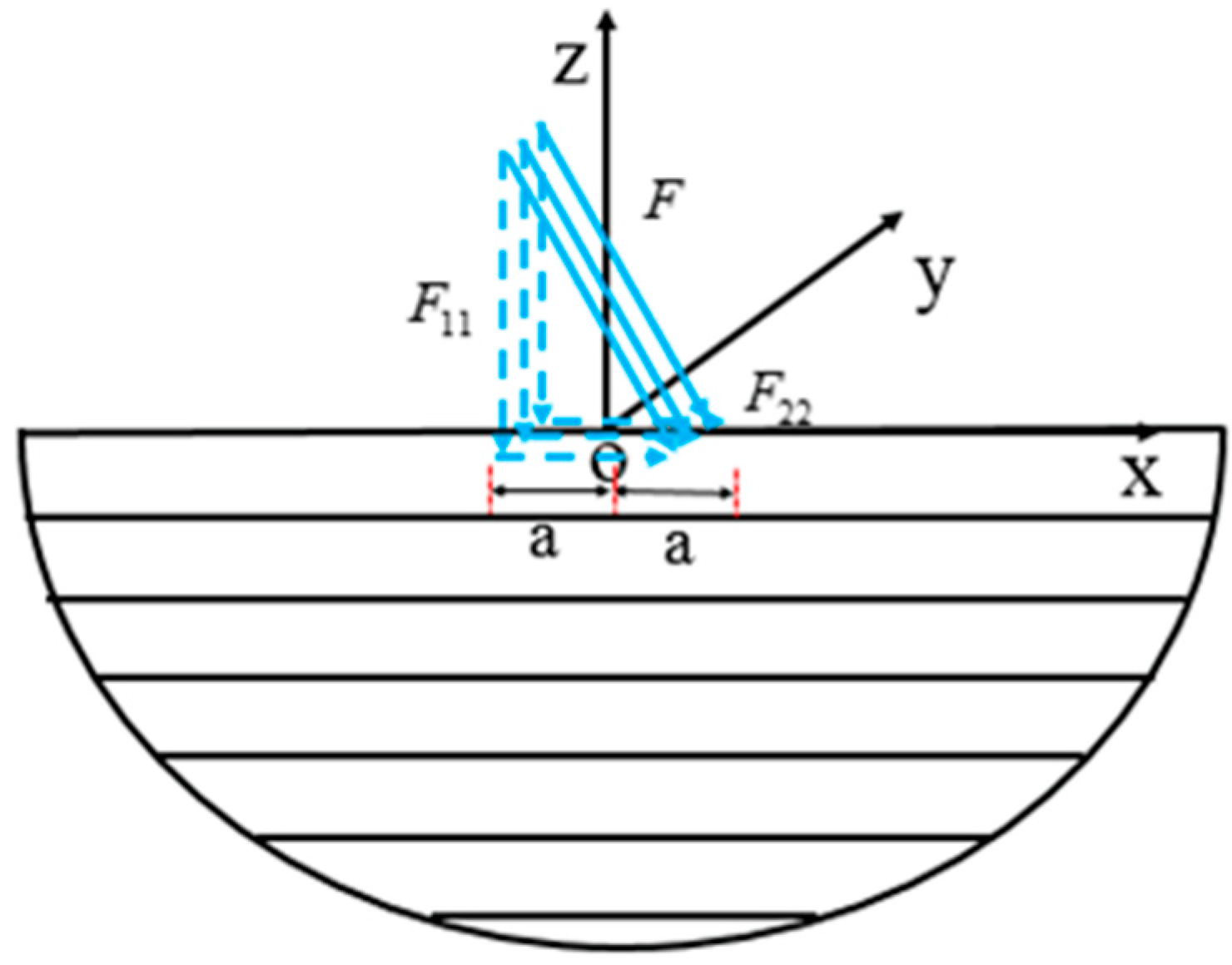
2.4. A Semi-Infinite Plane Subjected to Distributed Stresses in Any Direction

Given a semi-infinite body without physical force F, distributed stress in any direction is applied on its surface, which is decomposed into stress F₁₁ in the vertical direction and stress F₂₂ in the horizontal direction. The stress states at the area acting on the loading interface plane is shown in Figure 6. According to the previous analysis, the stress distribution for any direction can be deduced as follows:

$$\begin{array}{l}\Delta {\sigma }_F{}_x=\frac{F_{11}}{\pi }\left[K_1{A}_1{}^2\left(arc\tan \left(\frac{x+a}{A_{1}z}\right)-arc\tan \left(\frac{x-a}{A_{1}z}\right)\right)-K_2{A}_2{}^2\left(arc\tan \left(\frac{x+a}{A_{2}z}\right)-arc\tan \frac{x-a}{A_{2}z}\right)\right]\\ +\frac{F_{22}}{2\pi }\left[K_1{A}_1\cdot \ln \frac{{(x-a)}^2+A_1{}^2{z}^2}{{(x+a)}^2+{(A_{1}z)}^2}-K_2{A}_2\cdot \ln \frac{{(x-a)}^2+A_2{}^2{z}^2}{{(x+a)}^2+{(A_{2}z)}^2}\right]\end{array}$$

(23)

$$\begin{array}{l}\Delta {\sigma }_F{}_z=-\frac{F_{11}}{\pi }\left[K_1\left(arc\tan \left(\frac{x+a}{A_{1}z}\right)-arc\tan \left(\frac{x-a}{A_{1}z}\right)\right)-K_2\left(arc\tan \left(\frac{x+a}{A_{2}z}\right)-arc\tan \frac{x-a}{A_{2}z}\right)\right]\\ -\frac{F_{22}}{2\pi }\left[\frac{K_1}{A_1}\cdot \ln \frac{{(x-a)}^2+A_1{}^2{z}^2}{{(x+a)}^2+{(A_{1}z)}^2}-\frac{K_2}{A_2}\cdot \ln \frac{{(x-a)}^2+A_2{}^2{z}^2}{{(x+a)}^2+{(A_{2}z)}^2}\right]\end{array}$$

(24)

$$\begin{array}{l}{\tau }_F{}_{xz}=-\frac{F_{11}}{\pi }\left[\begin{array}{l}{K}_1{A}_1\left[\ln {\left({\left(x+a\right)}^2+{\left(A_{1}z\right)}^2\right)}^{1/2}-\ln {\left({\left(x-a\right)}^2+{\left(A_{1}z\right)}^2\right)}^{1/2}\right]-\\ K_2{A}_2\left[\ln {\left({\left(x+a\right)}^2+{\left(A_{2}z\right)}^2\right)}^{1/2}-\ln {\left({\left(x-a\right)}^2+{\left(A_{2}z\right)}^2\right)}^{1/2}\right]\end{array}\right]+\\ \frac{F_{22}}{\pi }\left[K_1\left(a\tan \frac{x-a}{A_{1}z}-a\tan \frac{x+a}{A_{1}z}\right)-K_2\left(a\tan \frac{x-a}{A_{2}z}-a\tan \frac{x+a}{A_{2}z}\right)\right]\end{array}$$

(25)

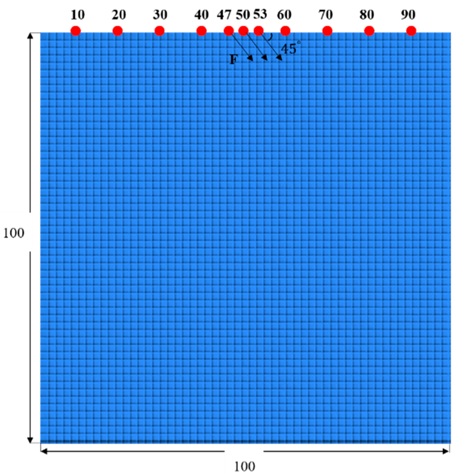
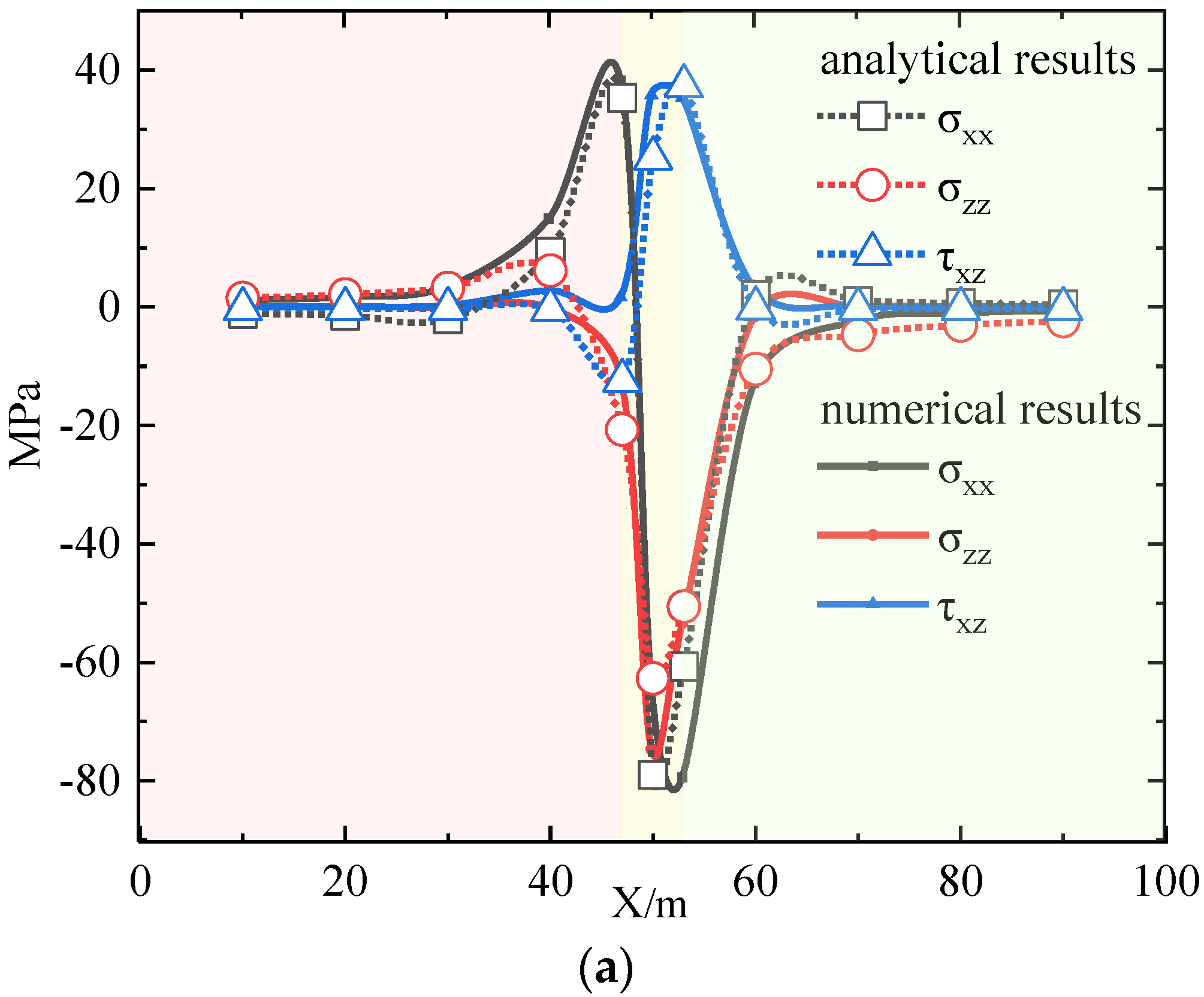
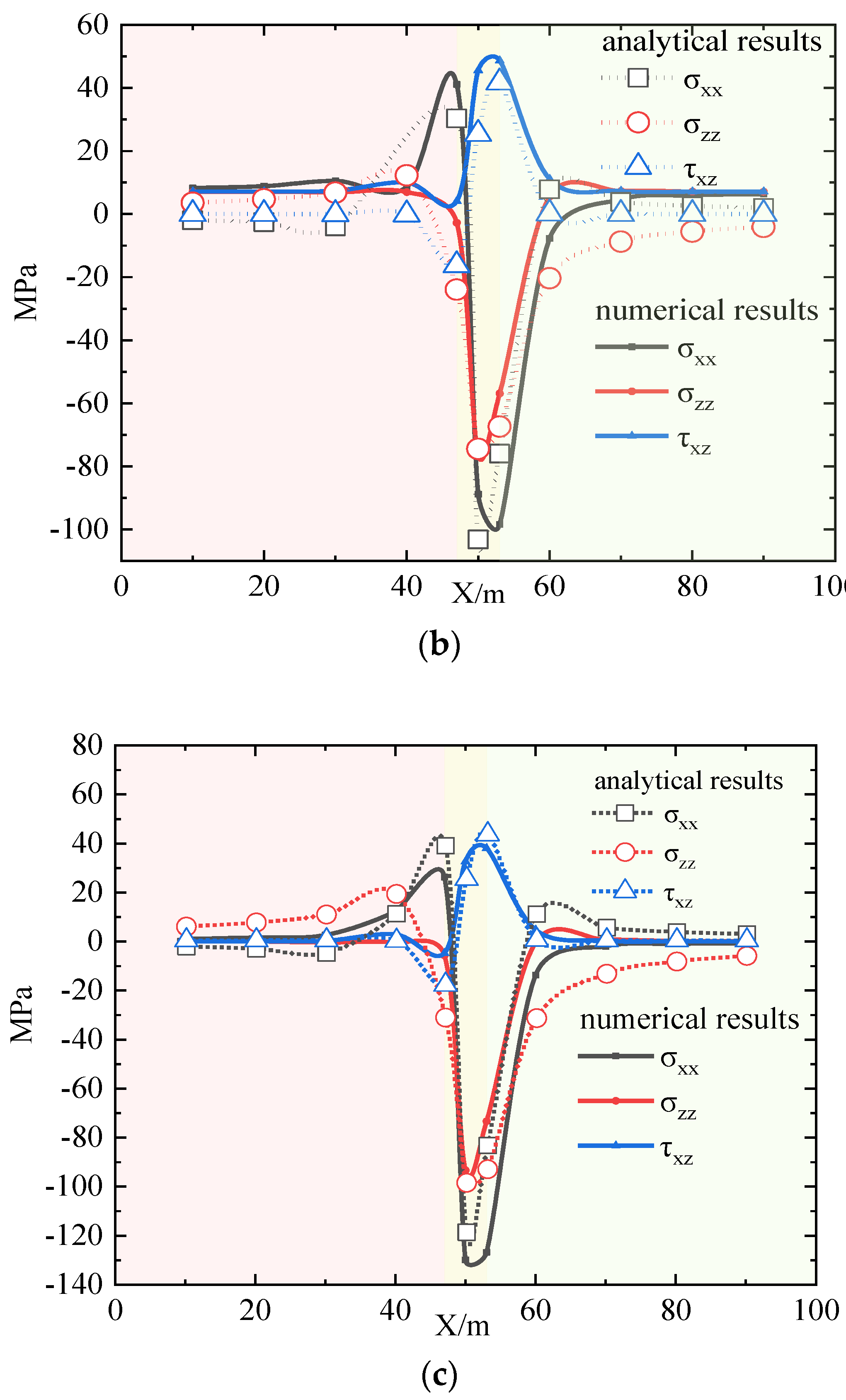
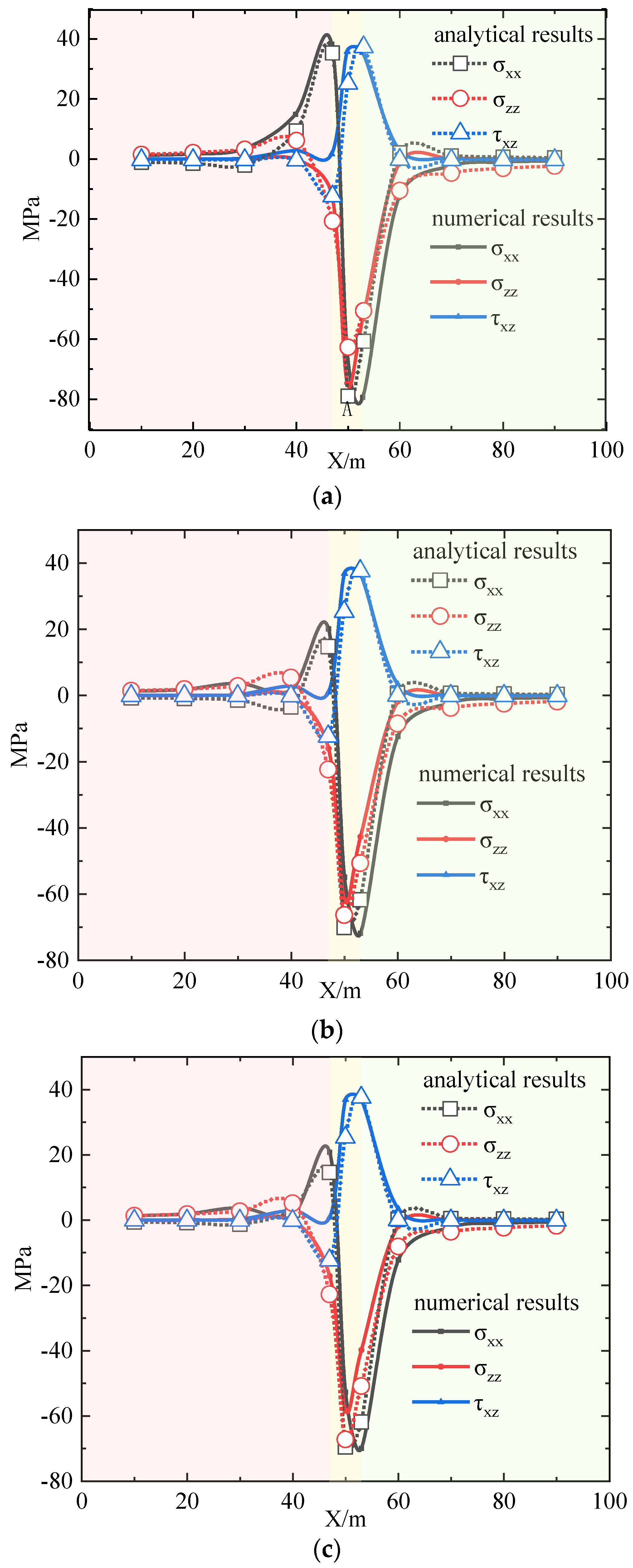
3. Verification against Numerical Simulations

To verify the proposed analytical solutions under distributed loading in any direction, a model is established with FLAC. The dimensions are 100 m, and the material parameters are shown in

Table 1. Parameters of the model.

Model	Length of the Side/m	γ/(kg/m3)	E1/GPa	E2/GPa	μ1	μ2	G/GPa
Parameters	100	2500	3	3	0.3	0.3	1.15

. The value of the distributed loading is $7\sqrt{2} \times 10\mathrm{MPa}$, and it is applied on the top of transversely isotropic floor rock at an angle of 45° to the horizontal plane to analyze the effect of the loading direction on the stress distribution of the model. The 11 measuring points and their positions in the numerical model are shown in Figure 7. The initial time step is $0.5 \mathsf{\mu }\mathrm{s}$, the maximum time is $1 \mathsf{\mu }\mathrm{s}$, and the relative and absolute tolerances during the calculation are $1e-5$. It has been noted that the time step was reasonable enough to guarantee the convergence and resolution accurately.

Prior to stress redistribution under different coefficients, a logical way to validate an analytical solution is to compare them with numerical solutions. Figure 8 shows several results of comparing the distribution of the stress fields based on the numerical simulation, accounting for the various values of the elastic moduli. To illustrate the factor (E) that affects the stress distribution, take ${\mu }_1={\mu }_2=0.3$, as $G_2$ is related to ${\mu }_1$, ${\mu }_2$, $E_1$, and $E_2$; given that $E_1=3\mathrm{GPa}$ set $E_1/E_2$ as 1.0, 2.0, and 3.0, respectively, and get the same depth (z = 1 m) distribution of ${\sigma }_{\mathrm{z}}$, ${\sigma }_{\mathrm{x}}$, and ${\tau }_{\mathrm{xz}}$, as shown in Figure 8. It indicates that the results, in terms of distributed stresses based on the proposed analytical solution for the transversely isotropic floor rock mass when compared with the numerical simulation, found that numerical solutions align favorably with the analytical solution, even though the amplitude of stress is not captured. From Figure 8a, it is observed that if the analytical solution is applied to the transversely isotropic floor rock mass, horizontal stress increases when x ≤ 47, then it undergoes the region in which there is an obvious decline until the peak stress is reached, corresponding to an overall decrease due to stress applied. For the case of x > 53, it shows a tendency to increase. In addition, vertical stress shows a sudden decrease and then rebounds, and it can be seen that the changes of shear stress are the exact opposite of vertical stress in Figure 8. Overall, the stress of an analytical solution is slightly greater than that of numerical simulations when x ≤ 47. On the contrary, the value of an analytical solution tends to be less than that of numerical simulations when x > 53. The reason for this phenomenon may be attributed to the influences of the model mesh. The results confirm the validity of the proposed solution, which can be utilized to estimate the stress distribution under distributed loading in an arbitrary direction.

The numerical model utilized in the discussion in this section might have been the same as that on the segment but for the elastic modulus and Poisson’s ratio. Take $E_1=E_2=3\mathrm{GPa}$, as $G_2$ is related to ${\mu }_1$, ${\mu }_2$, $E_1$, and $E_2$, given ${\mu }_1=0.3$ set ${\mu }_1/{\mu }_2$ as 1.0, 2.0 and 3.0, respectively, and obtain the same depth (z = 1 m) distribution of ${\sigma }_{\mathrm{z}}$, ${\sigma }_{\mathrm{x}}$, and ${\tau }_{\mathrm{xz}}$, as shown in Figure 9. It is denoted that there is very little difference between them, which indicates the proposed solution is feasible to obtain the stress concentration zone induced by stress redistribution with certain accuracy.

In conclusion, it is observed that there are some differences at the edge of the loading area in terms of the variation trend more specifically, which may be due to tension effects of the numerical model grid. Comparisons of results confirmed the validity of the proposed analytical solution, which is effective for capturing the characters of rock mass.

4. The Transverse Isotropic Stress Distribution Law

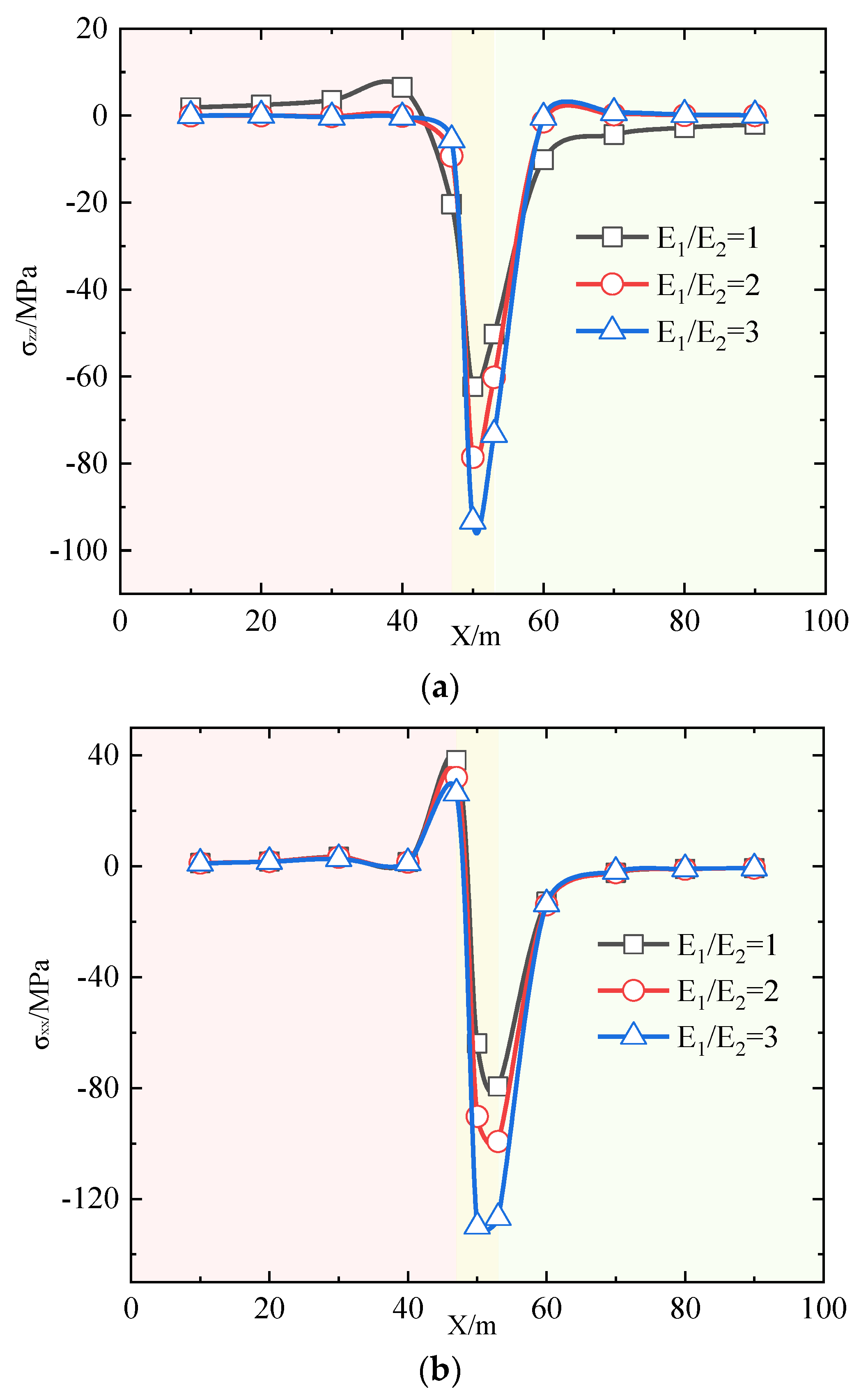
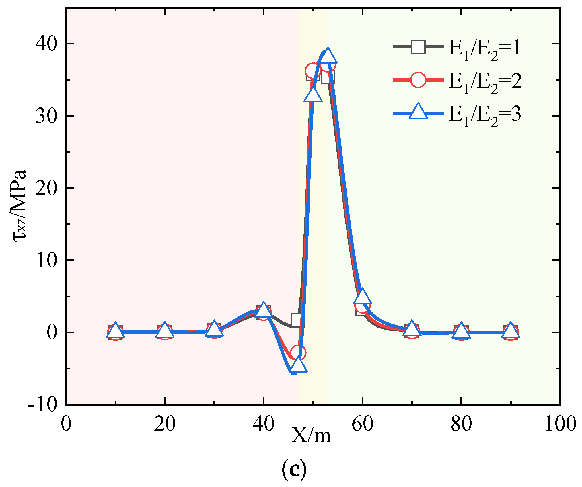
4.1. The Effect of E₁/E₂ on Stress Distribution

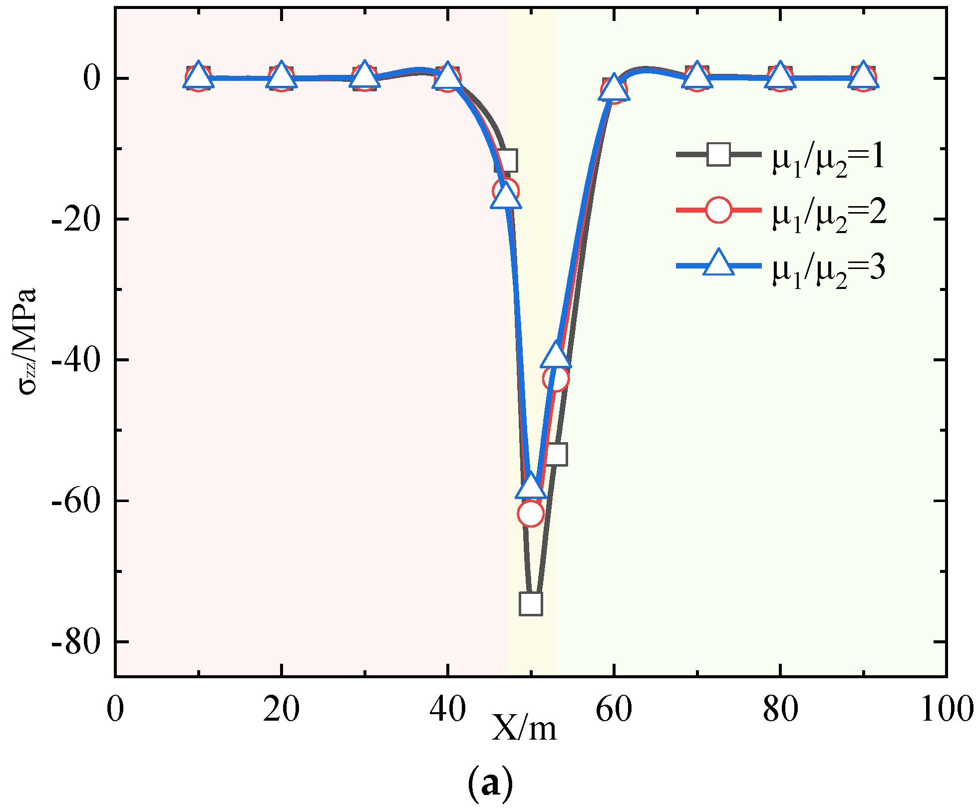
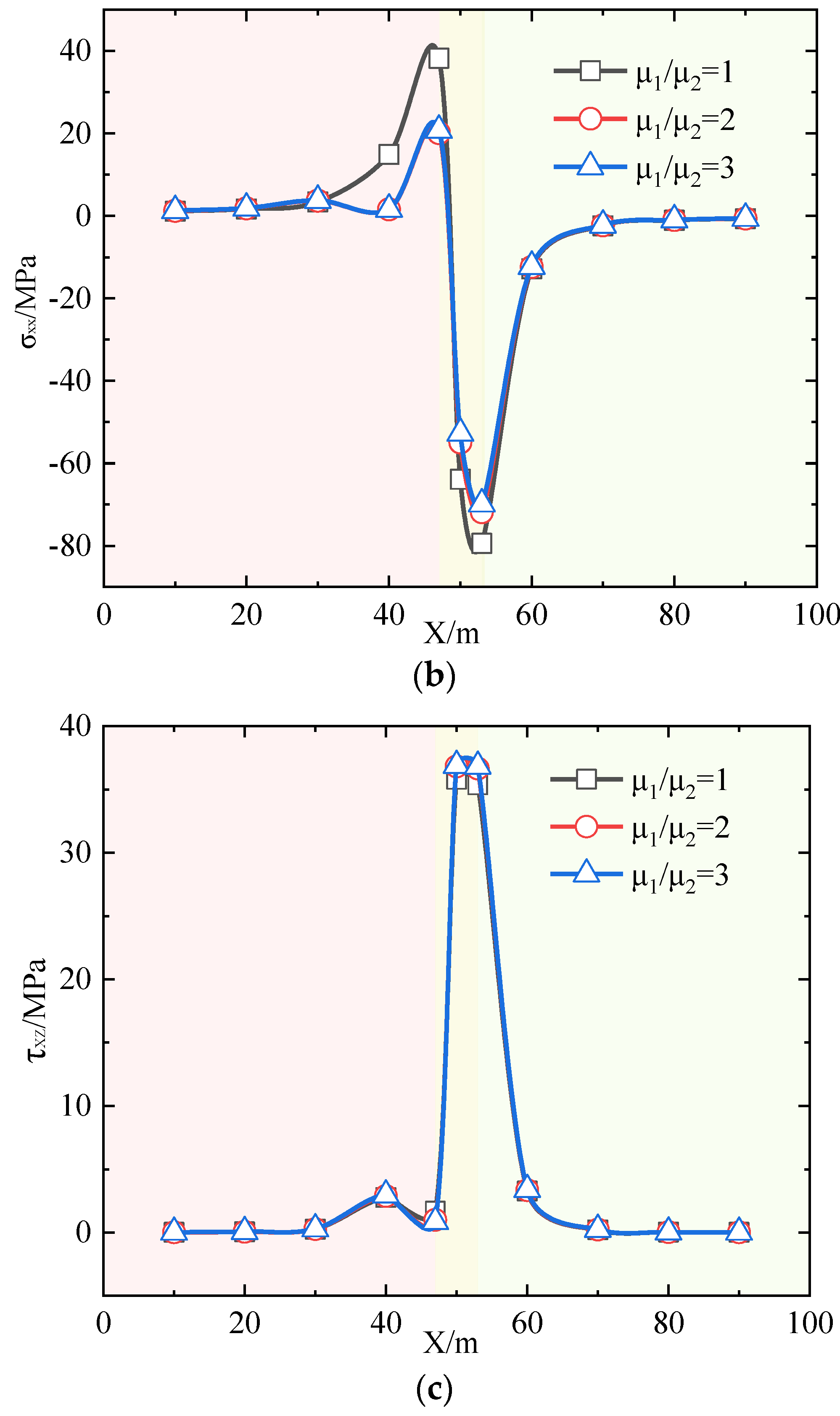
As can be seen from Figure 10a, the curve displayed a positive and negative stage. Obvious stress concentration is formed in the loading area, in which the value reached the peak stress, then it attenuates with the stress propagation along the X [46]. It is observed that with the increasing values of E₁/E₂, the magnitude of stress became bigger. The peak stress values are 62, 78, and 93 MPa, corresponding to the values of E₁/E₂ of 1, 2, and 3, respectively. This is due to stress that may be prone to propagation easily under higher values of $E_1/E_2$. As shown in Figure 10b, the peak stress of horizontal stress increases with the value, denoting the increase of the stress concentration with the value. Figure 10c shows that the corresponding peak values of the shear stress are 35, 37, and 38 MPa. Thus, the values of E₁/E₂ cannot be neglected to quantify the effect of stress concentration.

4.2. The Effect of μ₁/μ₂ on Stress Distribution

As shown in Figure 11, the effect of the anisotropy of Poisson’s ratio on the distribution of stress is opposite to that of elastic moduli. When increasing Poisson’s ratio anisotropy, the magnitude of the stress becomes even smaller. The peak stress values are 74, 61, and 58 MPa, which correspond to the values of μ₁/μ₂ of 1, 2, and 3, respectively. As can be seen from Figure 11b, the peak values of horizontal stress are determined as 79, 71, and 69 MPa which correspond to the values of μ₁/μ₂, respectively. This may be attributed to the difference of the deformation parameters of parallel planes and vertical planes. As shown in Figure 11c, it is noted that there are little differences of variation trends among them in terms of the values of μ₁/μ₂, suggesting that both the peak stress and wave velocity do not vary very much. In addition, the anisotropy of Poisson’s ratio has a great influence on the vertical stress and horizontal stress, but the influence on the shear stress is negligible.

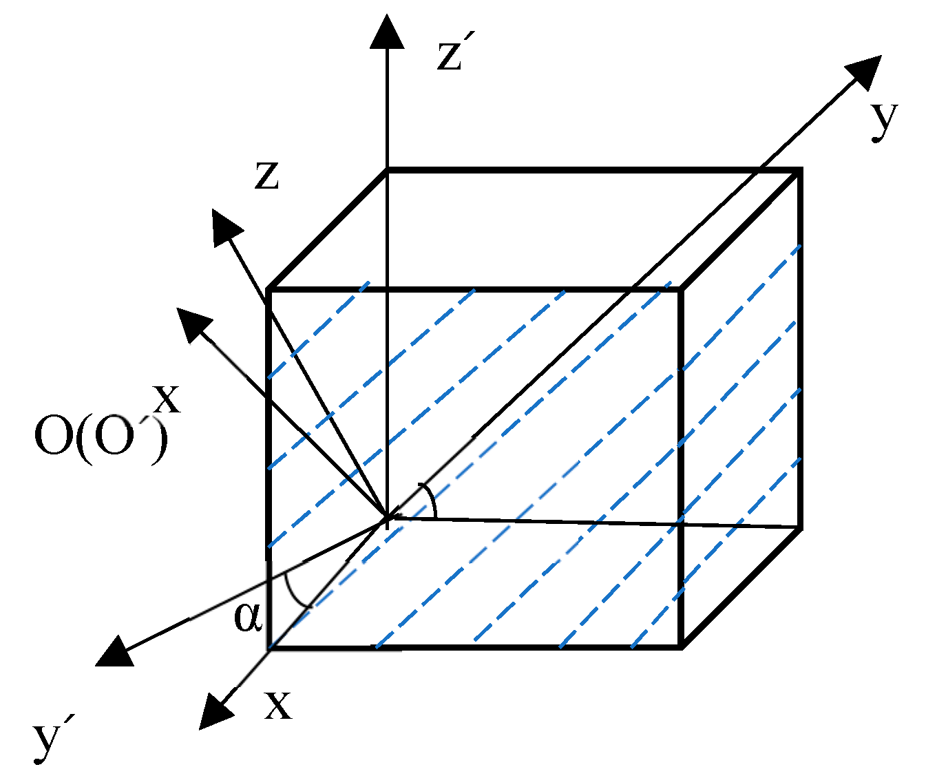
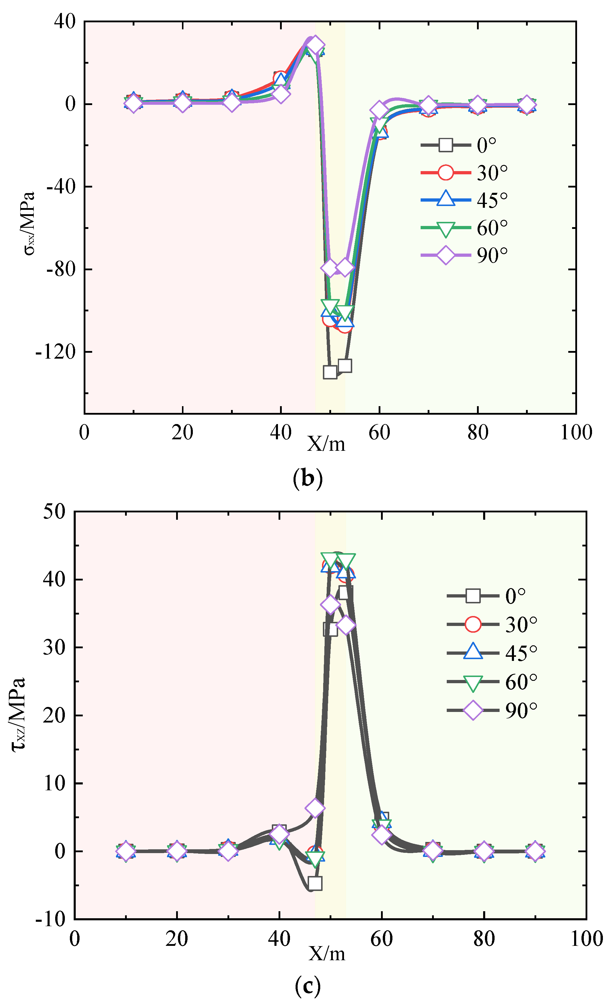
4.3. The Effect of the Formation Dip Angle on Stress Distribution

In fact, isotropic planes often incline due to long-term geological tectonics, as shown in Figure 12. The coordinate plane OX′Y′ is consistent with isotropic planes, while plane OXY is the horizontal plane, θ is the inclination angle of the isotropic plane, and α is the angle between the y′ axis and the x axis clockwise. Equation (28) shows the constitutive relation of the model in OX′Y′Z′ [47,48,49].

$$\left\{{\epsilon }^{\prime }\right\}=\left[A^{\prime }\right]\left\{{\sigma }^{\prime }\right\}$$

(26)

When the isotropic plane is tilted, the elastic matrix of the isotropic foundation in the axial coordinate system is:

$$A^{\prime }=Q^{T}AQ$$

(27)

where [A] is the elastic matrix in the positive axis coordinate system, and [Q] is the transformation matrix of elastic parameters

$$Q=\left[\begin{array}{cccccc}{\sin }^2\alpha & {\cos }^2\alpha & 0& 0& 0& -\sin 2\alpha \\ {\cos }^2\theta {\cos }^2\alpha & {\cos }^2\theta {\sin }^2\alpha & {\sin }^2\theta & -\sin 2\theta \sin \alpha & -\sin 2\theta \cos \alpha & \sin 2\alpha {\cos }^2\theta \\ {\sin }^2\theta {\cos }^2\alpha & {\sin }^2\theta {\sin }^2\alpha & {\cos }^2\theta & \sin 2\theta \sin \alpha & \sin 2\theta \cos \alpha & \sin 2\alpha {\sin }^2\theta \\ -\frac{1}{2}\sin 2\theta {\cos }^2\alpha & -\frac{1}{2}\sin 2\theta {\sin }^2\alpha & \frac{1}{2}\sin 2\theta & -\cos 2\theta \sin \alpha & -\cos 2\theta \cos \alpha & -\frac{1}{2}\sin 2\alpha \sin 2\theta \\ -\frac{1}{2}\sin \theta \sin 2\alpha & \frac{1}{2}\sin \theta \sin 2\alpha & 0& \cos \theta \cos \alpha & -\cos \theta \sin \alpha & \cos 2\alpha \sin \theta \\ \frac{1}{2}\cos \theta \sin 2\alpha & -\frac{1}{2}\cos \theta \sin 2\alpha & 0& \sin \theta \cos \alpha & -\sin \theta \sin \alpha & -\cos 2\alpha \cos \theta \end{array}\right]$$

(28)

In Figure 13a, the value of the vertical stress increases when the formation dip angle increases from 0° to 90°, while the opposite trend can be observed in Figure 13b,c. The greater the formation dip angle is, the lower the value of horizontal stress and shear stress. It can be seen that the formation dip angle has prominent effects on the distribution of the stress. The relationship is due to the changes of the formation dip, and the direction of stresses deflects and forms some range of stress redistribution.

5. Conclusions

In this paper, the distribution stress of transversely isotropic elastic half-plane surfaces subjected to distributed forces in any direction were investigated. The stress fields were determined, and the effects of the Young’s modulus, Poisson’s ratio, and the formation dip angle were taken into consideration in the elastic analysis. The accuracy and applicability of the analytical solutions proposed were examined and clarified by calculating some problems. From the analysis conducted, the following conclusions can be obtained:

(1) The analytical solution of transversely isotropic elastic half-plane surfaces subjected to distributed loading in any direction was proposed, and compared with the numerical solution, the two were in good agreement, which verifies the correctness of the analytical solution of transversely isotropic rock stress deduced in this paper.

(2) The stress concentration was closely related to the loading area, when Poisson’s ratio stayed the same with the increase of Young’s modulus anisotropy ratio, and the concentration degree of horizontal stress, vertical stress, and shear stress on the transversely isotropic plate had a 40%, 20%, and 3% increase in degree compared to that of the isotropic plate. However, with Young’s modulus and the increase of Poisson’s ratio, the concentration degree of vertical stress, horizontal stress, and shear stress on the transverse isotropic plate slightly decreased by 15%, 10%, and 4%, respectively.

(3) Along with the increasing value of the dip angle of layered rock mass, the vertical stress in the rock layer presented a slightly upward tendency, while the horizontal stress and shear stress decreased gradually.

(4) The proposed solution can be used to predict in situ stress. The stability of the working field is maintained after support, which can be further popularized and applied to related fields.

As a result, the analytical solution and numerical simulation can be capable of characterizing the transversely isotropic layers. However, in this study, the new findings are limited to homogeneous transversely isotropic half-space. In the future, the quantification of stress distributions in an inhomogeneous transversely isotropic half-space should be further studied.

References

1. Gatelier, N.; Pellet, F.; Loret, B. Mechanical damage of an anisotropic porous rock in cyclic triaxial tests. Int. J. Rock Mech. Min. Sci. 2002, 39, 335–354. [Google Scholar] [CrossRef]
2. Xu, G.; He, C.; Wang, X. Mechanical behavior of transversely isotropic rocks under uniaxial compression governed by micro-structure and micro-parameters. Bull. Eng. Geol. Environ. 2020, 79, 1979–2004. [Google Scholar] [CrossRef]
3. Shang, J.; Duan, K.; Gui, Y.; Handley, K.; Zhao, Z. Numerical investigation of the direct tensile behaviour of laminated and transversely isotropic rocks containing incipient bedding planes with different strengths. Comput. Geotech. 2017, 104, 373–388. [Google Scholar] [CrossRef] [Green Version]
4. Xu, G.W.; He, C.; Chen, Z.Q.; Su, A. Transverse Isotropy of Phyllite under Brazilian Tests: Laboratory Testing and Numerical Simulations. Rock Mech. Rock Eng. 2018, 51, 1111–1135. [Google Scholar] [CrossRef]
5. Nathan, D.; Morteza, N.; Benot, V.; Amann, F.; Giulio, M. On the link between fracture toughness, tensile strength, and fracture process zone in anisotropic rocks. Eng. Fract. Mech. 2018, 201, 56–79. [Google Scholar] [CrossRef]
6. Aliabadian, Z.; Zhao, G.F.; Russell, A.R. Crack development in transversely isotropic sandstone discs subjected to Brazilian tests observed using digital image correlation. Int. J. Rock Mech. Min. Sci. 2019, 119, 211–221. [Google Scholar] [CrossRef]
7. Li, K.; Cheng, Y.; Yin, Z.-Y.; Han, D.; Meng, J. Size effects in a transversely isotropic rock under brazilian tests: Laboratory testing. Rock Mech. Rock Eng. 2020, 53, 1–20. [Google Scholar] [CrossRef]
8. Li, L.; Aubertin, M. A crack-induced stress approach to describe the tensile strength of transversely isotropic rocks. Can. Geotech. J. 2002, 39, 1–13. [Google Scholar] [CrossRef]
9. Pietruszczak, S.; Mroz, Z. Formulation of anisotropic failure criteria incorporating a microstructure tensor. Comput. Geotech. 2002, 6, 105–112. [Google Scholar] [CrossRef]
10. Togashi, Y.; Kikumoto, M.; Tani, K. Determining anisotropic elastic parameters of transversely isotropic rocks through single torsional shear test and theoretical analysis. J. Pet. Sci. Eng. 2018, 169, 184–199. [Google Scholar] [CrossRef]
11. Mambou, L.L.; Ngueyep, N.; Dop, J. Numerical investigations of stresses and strains redistribution around the tunnel: Influence of transverse isotropic behavior of granitic rock, in situ stress and shape of tunnel. J. Min. Sci. 2015, 51, 497–505. [Google Scholar] [CrossRef]
12. Song, I.; Suh, M.; Woo, Y.K.; Hao, T. Determination of the elastic modulus set of foliated rocks from ultrasonic velocity measurements. Eng. Geol. 2004, 72, 293–308. [Google Scholar] [CrossRef]
13. Wang, C.D.; Tzeng, C.S.; Pan, E.; Liao, J.J. Displacements and stresses due to a vertical point load in an inhomogeneous transversely isotropic half-space. Int. J. Rock Mech. Min. Sci. 2003, 40, 667–685. [Google Scholar] [CrossRef]
14. Vashishth, A.K.; Poonam, K. Wave propagation along a cylindrical borehole in an anisotropic poroelastic solid. Geophys. J. Int. 2005, 161, 295–302. [Google Scholar] [CrossRef] [Green Version]
15. Li, W.; Schmitt, D.R.; Zou, C.; Chen, X. A program to calculate pulse transmission responses through transversely isotropic media. Comput. Geosci. 2018, 114, 59–72. [Google Scholar] [CrossRef]
16. Hu, S.; Tan, Y.; Zhou, H.; Ru, W.; Ning, J.; Wang, J.; Huang, D.; Li, Z. Anisotropic modeling of layered rocks incorporating planes of weakness and volumetric stress. Energy Sci. Eng. 2019, 8, 789–803. [Google Scholar] [CrossRef]
17. Motra, H.B.; Mager, J.; Ismail, A.; Wuttke, F.; Rabbel, W.; Köhn, D.; Thorwart, M.; Simonetta, C.; Costantino, N. Determining the influence of pressure and temperature on the elastic constants of anisotropic rock samples using ultrasonic wave techniques. J. Appl. Geophys. 2018, 159, 715–730. [Google Scholar] [CrossRef]
18. Nunes, L.S.; Laura, A. A new method for determination of transverse isotropic orientation and the associated elastic parameters for intact rock. Int. J. Rock Mech. Min. Sci. 2002, 39, 257–273. [Google Scholar] [CrossRef]
19. Simanjuntak, T.D.Y.F.; Marence, M.; Schleiss, A.J.; Mynett, A.E. The Interplay of In Situ Stress Ratio and Transverse Isotropy in the Rock Mass on Prestressed Concrete-Lined Pressure Tunnels. Rock Mech. Rock Eng. 2016, 49, 1–22. [Google Scholar] [CrossRef]
20. Jin, W.; Arson, C. Anisotropic nonlocal damage model for materials with intrinsic transverse isotropy. Int. J. Solids Struct. 2018, 139, 29–42. [Google Scholar] [CrossRef]
21. Que, X.C.; Zhu, Z.D.; Lu, W.B. Anisotropic constitutive model of pentagonal prism columnar jointed rock mass. Bull. Eng Geol. Environ. 2020, 79, 269–286. [Google Scholar] [CrossRef]
22. Xu, D.-P.; Feng, X.-T.; Chen, D.-F.; Zhang, C.-Q.; Fan, Q.-X. Constitutive representation and damage degree index for the layered rock mass excavation response in underground openings. Tunn. Undergr. Space Technol. Inc. Trenchless Technol. Res. 2017, 64, 133–145. [Google Scholar] [CrossRef]
23. Hu, J.; Cao, J.; Wang, H.; Wang, X.; Tian, R. 3D P-wave traveltime computation in transversely isotropic media using layer-by-layer wavefront marching. Geophys. Prospect. 2018, 66, 1303–1314. [Google Scholar] [CrossRef]
24. Vu, T.M.; Sulem, J.; Subrin, D.; Monin, N. Semi-Analytical Solution for Stresses and Displacements in a Tunnel Excavated in Transversely Isotropic Formation with Non-Linear Behavior. Rock Mech. Rock Eng. 2012, 46, 213–229. [Google Scholar] [CrossRef]
25. Mahjoub, M.; Rouabhi, A.; Tijani, M.; Granet, S. An approach to model the mechanical behavior of transversely isotropic materials. Int. J. Numer. Anal. Methods Geomech. 2016, 40, 942–961. [Google Scholar] [CrossRef]
26. Olsen-Kettle, L. Using ultrasonic investigations to develop anisotropic damage models for initially transverse isotropic materials undergoing damage to remain transverse isotropic. Int. J. Solids Struct. 2018, 138, 155–165. [Google Scholar] [CrossRef] [Green Version]
27. Mahabadi, O.K.; Lisjak, A.; Munjiza, A.; Grasselli, G. New combined finite-discrete element numerical code for geomechanical applications. Int. J. Geomech. 2012, 12, 676–688. [Google Scholar] [CrossRef]
28. Chen, J.; Lan, H.; Macciotta, R.; Wu, Y.; Li, Q.; Zhao, X. Anisotropy rather than transverse isotropy in Longmaxi shale and the potential role of tectonic stress. Eng. Geol. 2018, 247, 38–47. [Google Scholar] [CrossRef]
29. Tonon, F.; Amadei, B. Effect of Elastic Anisotropy on Tunnel Wall Displacements behind a Tunnel Face. Rock Mech. Rock Eng. 2002, 35, 141–160. [Google Scholar] [CrossRef]
30. Kong, S.C. Interaction between transverse isotropy rock slope and supporting structure. J. Cent. South Univ. Technol. 2008, 15, 415–423. [Google Scholar]
31. Fang, X.D. A revisit to the Lekhnitskii-Amadei solution for borehole stress calculation in tilted transversely isotropic media. Int. J. Rock Mech. Min. Sci. 2018, 104, 113–118. [Google Scholar] [CrossRef]
32. Meier, T.; Rybacki, E.; Backers, T.; Dresen, G. Influence of Bedding Angle on Borehole Stability: A Laboratory Investigation of Transverse Isotropic Oil Shale. Rock Mech. Rock Eng. 2015, 48, 1535–1546. [Google Scholar] [CrossRef]
33. Li, Y.; Weijermars, R. Wellbore stability analysis in transverse isotropic shales with anisotropic failure criteria. J. Pet. Sci. Eng. 2019, 176, 982–993. [Google Scholar] [CrossRef]
34. Liang, R.Y.; Shatnawi, E.S. Estimating Subgrade Reaction Modulus for Transversely Isotropic Rock Medium. J. Geotech. Geoenviron. Eng. 2010, 136, 1077–1085. [Google Scholar] [CrossRef]
35. Tang, X. Determining formation shear-wave transverse isotropy from borehole Stoneley-wave measurements. Geophysics 2003, 68, 118–126. [Google Scholar] [CrossRef]
36. Chen, Y.F.; Ai, Z.Y. Viscoelastic analysis of transversely isotropic multilayered porous rock foundation by fractional Poyting-Thomson model. Eng. Geol. 2019, 264, 105327. [Google Scholar] [CrossRef]
37. Ai, Z.Y.; Chen, Y.F. FEM-BEM coupling analysis of vertically loaded rock-socketed pile in multilayered transversely isotropic saturated media. Comput. Geotech. 2020, 120, 103437. [Google Scholar] [CrossRef]
38. Qi, Z.; Choo, J.; Borja, R. On the preferential flow patterns induced by transverse isotropy and non-Darcy flow in double porosity media. Comput. Methods Appl. Mech. Eng. 2019, 353, 70–592. [Google Scholar] [CrossRef]
39. Jiang, Q.; Feng, X.-T.; Hatzor, Y.; Hao, X.-J.; Li, S.-J. Mechanical anisotropy of columnar jointed basalts: An example from the Baihetan hydropower station, China. Eng. Geol. 2014, 175, 35–45. [Google Scholar] [CrossRef]
40. Chen, C.S.; Chen, C.H.; Pan, E. Three-dimensional stress intensity factors of a central square crack in a transversely isotropic cuboid with arbitrary material orientations. Eng. Anal. Bound. Elem. 2009, 33, 128–136. [Google Scholar] [CrossRef]
41. Xu, D.-P.; Feng, X.-T.; Cui, Y.-J.; Jiang, Q. Use of the equivalent continuum approach to model the behavior of a rock mass containing an interlayer shear weakness zone in an underground cavern excavation. Tunn. Undergr. Space Technol. Inc. Trenchless Technol. Res. 2015, 47, 35–51. [Google Scholar] [CrossRef]
42. Li, X.; Lei, X.; Li, Q. Response of Velocity Anisotropy of Shale under Isotropic and Anisotropic Stress Fields. Rock Mech. Rock Eng. 2017. [Google Scholar] [CrossRef]
43. Youn-Kyou, L. Stress distribution under line load in transversely isotropic rock mass. Tunn. Undergr. Space 2005, 15, 288–295. [Google Scholar]
44. Ai, Z.-Y.; Cang, N.-R.; Han, J. Analytical layer-element solutions for a multi-layered transversely isotropic elastic medium subjected to axisymmetric loading. J. Zhejiang Univ. A 2012, 13, 9–17. [Google Scholar] [CrossRef]
45. Wang, C.D.; Wang, W.J.; Lee, T.C. Three-dimensional buried non-linearly varying triangular loads on a transversely isotropic half-space. Int. J. Solids Struct. 2004, 41, 3013–3030. [Google Scholar] [CrossRef]
46. Liao, J.J.; Hu, T.B.; Wang, C.D. Elastic solutions for an inclined transversely isotropic material due to three-dimensional point loads. J. Mech. Mater. Struct. 2008, 3, 1521–1547. [Google Scholar] [CrossRef]
47. Xu, G.; He, C.; Chen, Z.; Yang, Q. Transversely isotropic creep behavior of phyllite and its influence on the long-term safety of the secondary lining of tunnels. Eng. Geol. 2020, 278, 105834. [Google Scholar] [CrossRef]
48. Shen, P.; Tang, H.; Zhang, B.; Ning, Y.; He, C. Investigation on the fracture and mechanical behaviors of simulated transversely isotropic rock made of two interbedded materials. Eng. Geol. 2021, 286, 106058. [Google Scholar] [CrossRef]
49. Aliabadian, Z.; Zhao, G.F.; Russell, A.R. An Analytical Study of Failure of Transversely Isotropic Rock Discs Subjected to Various Diametrical Loading Configurations. Procedia Eng. 2017, 191, 1194–1202. [Google Scholar] [CrossRef]
Figure 1. Transversely isotropic constitutive model.
Applsci 11 10476 g001
Figure 2. A transversely isotropic elastic half-plane surface subjected to vertically concentrated stress.
Applsci 11 10476 g002
Figure 3. Transversely isotropic elastic half-plane surface subjected to vertically distributed stress.
Applsci 11 10476 g003
Figure 4. Transversely isotropic elastic half-plane surface subjected to horizontally concentrated stress.
Applsci 11 10476 g004
Figure 5. Transversely isotropic elastic half-plane surface subjected to horizontally distributed stress.
Applsci 11 10476 g005
Figure 6. Transversely isotropic elastic half-plane surface subjected to distributed stress in any direction.
Applsci 11 10476 g006
Figure 7. Numerical model.
Applsci 11 10476 g007
Figure 8. Comparisons between the proposed solution and numerical results for the values of E1/E2. (a) E 1 / E 2 = 1   , (b) E 1 / E 2 = 2   , (c) E 1 / E 2 = 3   .
Applsci 11 10476 g008aApplsci 11 10476 g008b
Figure 9. Comparisons between the proposed solution and numerical results for the values of μ12. (a) μ 1 / μ 2 = 1 , (b) μ 1 / μ 2 = 2 , (c) μ 1 / μ 2 = 3 .
Applsci 11 10476 g009
Figure 10. Analytical results for different values of E1/E2. (a) vertical stress, (b) horizontal stress, (c) shear stress.
Applsci 11 10476 g010aApplsci 11 10476 g010b
Figure 11. Analytical results for the different values of μ12. (a) vertical stress, (b) horizontal stress, (c) shear stress.
Applsci 11 10476 g011aApplsci 11 10476 g011b
Figure 12. Transversely isotropic constitutive model with isotropic plane inclines.
Applsci 11 10476 g012
Figure 13. Analytical results for different values of formation dip. (a) vertical stress, (b) horizontal stress, (c) shear stress.
Applsci 11 10476 g013aApplsci 11 10476 g013b