
Skull Thickness Calculation Using Thermal Analysis and Finite Elements


1
Department of Informatics, Bingol University, Bingol 12000, Turkey
2
Department of Computer Engineering, Inonu University, Malatya 44280, Turkey
3
Department of Automated Mechanical Engineering, South Ural State University, Lenin Prosp. 76, 454080 Chelyabinsk, Russia
4
School of Mechanical and Design Engineering, University of Portsmouth, Portsmouth PO1 3DJ, UK
*
Author to whom correspondence should be addressed.
Appl. Sci. 2021, 11(21), 10483; https://0-doi-org.brum.beds.ac.uk/10.3390/app112110483
Submission received: 30 September 2021
/
Revised: 31 October 2021
/
Accepted: 5 November 2021
/
Published: 8 November 2021
Abstract
:In this study, the skull bone thicknesses of 150 patients ranging in age from 0 to 72 years were calculated using a novel approach (thermal analysis), and thickness changes were analyzed. Unlike conventional thickness calculation approaches (Beam Propagation, Hildebrand), a novel heat transfer-based approach was developed. Firstly, solid 3D objects with different thicknesses were modeled, and thermal analyses were performed on these models. To better understand the heat transfer of 3D object models, finite element models (FEM) of the human head have been reported in the literature. The FEM can more accurately model the complex geometry of a 3D human head model. Then, thermal analysis was performed on human skulls using the same methods. Thus, the skull bone thicknesses at different ages and in different genders from region to region were determined. The skull model was transferred to ANSYS, and it was meshed using different mapping parameters. The heat transfer results were determined by applying different heat values to the inner and outer surfaces of the skull mesh structure. Thus, the average thicknesses of skull regions belonging to a certain age group were obtained. With this developed method, it was observed that the temperature value applied to the skull was proportional to the thickness value. The average thickness of skull bones for men (frontal: 7.8 mm; parietal: 9.6 mm; occipital: 10.1 mm; temporal: 6 mm) and women (frontal: 8.6 mm; parietal: 10.1 mm; occipital: 10 mm; temporal: 6 mm) are given. The difference (10%) between men and women appears to be statistically significant only for frontal bone thickness. Thanks to the developed method, bone thickness information at any desired point on the skull can be obtained numerically. Therefore, the proposed method can be used to help pre-operative planning of surgical procedures.
1. Introduction
Since the human skull protects the brain, which is the most important part of our body, it is the most important bone structure making up our anatomy. This structure has important components such as the frontal, parietal, occipital, temporal, and sphenoidal components, and other small parts [1,2]. These components are connected by connection points called sutures. Skull bones are complex shapes and have different compositions. Understanding them thoroughly requires explaining the relationship between their functions and forms. Skull bone thickness differs between the genders [3,4]. Generally, a female skeleton tends to be smaller and less durable than a male skeleton. To better understand the mechanisms of head injuries, the mechanical properties of the skull are measured when an impact occurs [5] or when the skull is subjected to abnormal loads [6]. The mechanical resistance of the skull is highly dependent on skull thickness. Knowing the thickness of patient-specific skull sections for plastic surgery can save workload and time during surgical operations [7].
Most of the studies on skull bone thickness use archeological materials. Many studies have reported that skull thickness varies greatly from one person to another [8]. In studies, mechanical measurements are generally performed with digital calipers on skulls with limited measurement points [9]. Moreover, such existing methods have only been used in laboratory environments (in vitro) or under artificial conditions. However, the thickness of the skull bones has been evaluated in two-dimensional limited sections on the basis of computed tomography (CT) scan slices [10,11]. Another way to obtain thickness measurements is to create a three-dimensional (3D) model of the skull bone [12]. Modeling was performed on the basis of MRI data, which allowed the skull shape to be reconstructed, but this method also was not able to take into account the inner surface, and the skull thickness could not be evaluated at the desired level [13]. Skull thickness directly affects skull conductivity. The most important factor in epilepsy surgery is skull conductivity [14]. In a previous study, significant correlation information was obtained between skull thickness and skull conductivity [15]. Skull thickness is a very important factor in terms of skull deterioration and tendency to fracture [16]. The characterization of the thickness of the skull and understanding the manner in which this information changes with age are important steps in understanding the role of thickness in skull deterioration.
Current methods for measuring skull thickness in adults are based on taking measurements using a saw at predetermined points in the skull. However, these methods may not give correct information about skull thickness. To address this issue, a different method was proposed to measure the skull thickness of adults using standardized anatomical points [17]. In another study, an automated approach to measuring skull thickness using CT images to determine soft tissue locations was presented [18]. In addition, a method for measuring skull thickness using after-death skull CT images of children was developed [19]. However, since the skull growth rate in children is extremely variable in this method, it is very difficult to determine a standard point from which to start the measurements. The finite element model of the skull is used to study the biomechanics of traumatic brain injury, and it is highly dependent on head geometry. In a study conducted using this information, a skull database containing information on the age-specific development of children’s skulls was created with the help of the finite element model [20].
Hildebrand et al. proposed a method for defining the local thickness for an arbitrary structure without model assumptions [21]. According to this, the local thickness at the point of an arbitrary structure is determined by fitting maximal spheres to every point on the structure. The application of this theory led researchers to the development of a number of different application techniques due to its high computational costs. The disadvantage of the Hildebrand method is that it does not work directly on the 3D volume. The results obtained from the 2D projection of a 3D volume object are processed. With the Beam Propagation method, ultrasound measurements of beam-based thickness are performed [22]. In this method, phase aberrations and differences due to high levels of absorption occur. Poor focusing and higher energy loss occur, especially at higher ultrasound frequencies. The main issue faced by the Beam Propagation and Hildebrand methods that has not been addressed previously, and which could be important, is the inability of these methods to deal with 3D medical images and pediatric skulls. Not all state-of-the-art methods can do it, but in any case, it would be interesting to explain why this is the case, and whether this problem can be solved by FEM-based thermal analysis of CT images. It is possible to apply our method to all skull regions separately, and to subsequently combine their results. FEM-based thermal analysis provides more descriptive distance information about skull thickness through the Euclidean function.
Existing methods of measuring skull thickness in adults require improvement. Most of them do not give accurate results for pediatric skulls [23]. Therefore, a method that can accurately calculate both pediatric and adult skull thicknesses is required. In our study, both pediatric and adult skull thicknesses can be calculated numerically. There is currently no relevant literature investigating the evolution of skull thickness across all growth stages.
This paper proposes a fast and reliable method for determining skull thickness on the basis of CT images. In the proposed method, the thickness of the desired area of the skull can be calculated by using the finite element method and the thermal heat method, without the application of any surgical procedures. It should be pointed out that this feature makes the proposed method appropriate in scenarios where automatic determination of skull thickness is required. In the literature, there is no specific study in the field of head imaging presenting the use of the FEM and thermal heat methods together. Another gap seen in the literature is the lack of methods that can numerically calculate both pediatric and adult skull thicknesses. In our study, it is shown that the proposed method makes it easier to evaluate how skull thickness changes with age. Thus, owing to the generation of an effective skull mesh map with the finite element method, the bone thicknesses of all human skulls can be calculated, independently of gender and age.
The paper is structured as follows. In Section 2, the determination of the thickness of a solid object using the thermal analysis method is shown using ANSYS finite element software 2020 R1. In Section 3, comprehensive information about the skull images used in this paper is given. Then, the proposed skull bone thickness calculation method based on the proposed thermal analysis is described. Finally, Section 4 includes the experimental results and recommendations.
2. Materials and Methods
The main motivation of this study was to determine the thicknesses of the human skull taken on the basis of CT data using thermal analysis at different points. Thus, a method based on thermal analysis is presented for determining bone thickness. Three-dimensional solid models are produced to facilitate better understanding. Then, thermal analysis is applied to solid models covered with mesh.
2.1. Generating Solid 3D Models
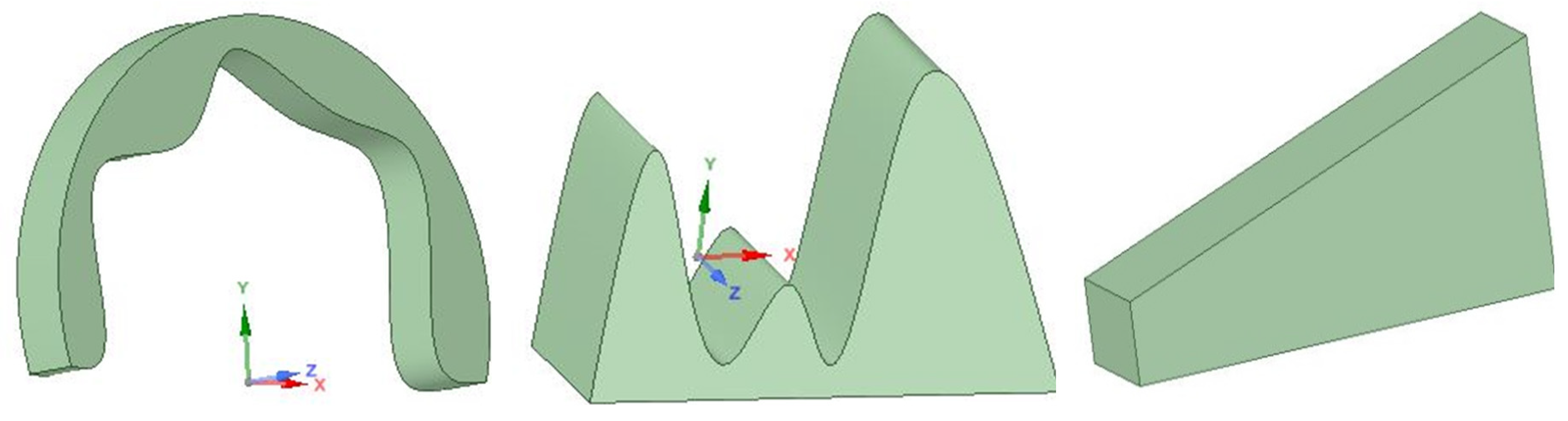
It is known that thermal analysis can be applied in order to develop solutions to different problems regarding objects. Especially in solid objects and systems operating based on heat, significant information about the system status can be obtained by using thermal analysis methods. In this section, various applications are presented in order to present the reader with information on how thermal analysis works. Thus, we aim to provide important information and explanations for the application of thermal analysis in skull bones. Models of 3D solids are highly suitable objects for this purpose. Three-dimensional solid model structures were created that are similar to the geometric structures of skulls. The thickness of these models varies at different coordinates, as is the case for the bone structure of skulls. These models were created using SpaceClaim software 2020 R1. Some of the 3D solid models are shown in Figure 1.
Human bones have heterogeneous and nonlinear structures. Therefore, it is difficult to assign material properties along each aspect of the bone. Although bone is an example of a natural composite material, its properties vary from one point to another [24]. In this study, we assume bone to be an isotropic material, and we aim to perform further analysis. The material properties used in similar analyses by other researchers are shown in Table 1.
In Table 1, the Young’s modulus is the initial slope of the stress–strain curve. The amount of matter per unit volume of the modeled objects also gives the density. The ratio of lateral stress to axial stress gives the Poisson value. The 3D objects were defined as anisotropic materials with the following properties: Young’s modulus: 380 MPa; and Poisson’s ratio: 0.22. With these selected values, solid models suitable for the bone structure of the human skull are created. Thus, the thermal analysis studies to be carried out will be performed using parameters that are suitable for applications on the human skull.
2.2. Mesh Generation Using the Finite Element Method
The finite element (FE) method is a numerical technique used to analyze various engineering problems [28,29,30,31]. This technique separates a large system into smaller and simpler parts, called finite elements. This method is increasingly frequently being applied to analyze bone structures [32]. FE can also be used to model complex geometries such as 3D solid models. The aim is to obtain reliable results with the least error and minimum calculation time, regardless of mesh size and density. Simulations were executed on a high-performance workstation with an Intel Core i7-6700 processor (3.40 GHz) and 16 GB RAM. Firstly, the created models are transferred to FE-based ANSYS. While designing the models, the anatomy of the skull was taken into account [33]. Then these solid models are meshed to prepare thermal analysis. The curvature and element size are adjusted to fit the model mesh, since the solid model has a curved structure, in order to maximize resemblance to the skull. The number of nodes and elements in a solid model varies depending on the size of the mesh. By using the sizing option under the mesh menu, the size of the element is selected as 1, 2, and 3 mm. As the mesh size gets smaller, the number of nodes and elements also increases. Table 2 shows the number of nodes, the number of elements, and the study time required, depending on the different element sizes of the meshed model. FE mesh models of three types with different levels were generated. During the analyses, it was determined that FE model-3 had the largest mesh size, but provided a reliable solution in terms of both time and number of elements. Therefore, we preferred the FE model-3 over the other two FE models (1 and 2), and used it in the subsequent analyses. Thanks to the improvement of the network and the use of the options available in the software, the network quality was increased, and optimal results were obtained. Figure 2 shows the meshed solid models with different numbers of nodes and elements.
2.3. Thermal Analysis of 3D Solid Models
Heat transfer is thermal energy that is in transition due to differences in spatial temperature. The most efficient method of heat transfer is conduction. This heat transfer method occurs whenever there is any temperature change within an object. In this case, energy is transferred from a high-temperature region to a low-temperature region.
The current equation of thermal conduction in continuous environments can be obtained on the basis of the principle of conservation of thermal energy. The application of the heat transfer relationship for systems with isotropic materials is as follows [34]:
where represents density, is the specific heat, is the environmental temperature, is the time, is the thermal conduction coefficient, and is the internal heat produced per volume.
The amount of heat transferred by convection is determined by Newton’s law of cooling, as follows:
where is the convection coefficient, is the temperature of the surface boundaries, and is the environmental temperature. The convection coefficient is a function of properties such as fluid velocity and surface roughness. Simplified formulas are available for calculating this coefficient [35].
In this section, thermal analysis of the modeled solid object is examined. Thus, we aim to carry out an experimental application in order to verify the application of the model for skull images. ANSYS Workbench-2020 software was used for analysis. The ANSYS Workbench interface consists of a toolbox, project diagram, toolbar, and menu bar. Two main types of thermal analysis are commonly used. These are steady-state thermal analysis and transient thermal analysis. Steady-state analysis is performed at a constant temperature, while transient thermal analysis is performed at varying temperatures. Steady-state thermal analysis is important for determining temperatures, heat fluxes, etc. In the steady-state method, a constant known heat flow is assumed to stream through an object [36]. Steady-state thermal analysis is used in this study. This type of analysis calculates the effect of a constant thermal load on a solid 3D object. To this end, thermal analysis is used to determine the temperature, thermal slope, heat flow rates, and heat flow in the object [37]. One of the important issues in creating 3D thermal models is to create appropriate boundary conditions. The steps for realizing the steady-state thermal analysis of a 3D structure are as follows: (1) the designed 3D model is taken; (2) the model is meshed; (3) the outside temperature is given a value other than 0 °C; and (4) 0 °C is applied to the entire inner surface as a constant heat source.
Since the modeled solid object contains experimental applications for the bone structure of the human skull, it was designed with different thicknesses. Temperature differences were analyzed by applying different amounts of heat to the interior and exterior surfaces. The temperature value of the inner surface was accepted as 0 °C. This process, which is applied to solid models, can also be applied to living human skulls (see Section 4). However, no direct thermal application is made to the skull of the living person. First, CT images taken from the person are converted into a model for thermal analysis. The internal and external surface temperature values of the skull that is turned into the model are unimportant, because at this stage, the focus is on the internal–external surface temperature differences. In this case, choosing 0 °C or a different value for the inner surface makes no difference. For the convenience of mathematical operations, the inner surface was accepted as being 0 °C. Thus, the heat value on the outer surface will directly provide the temperature difference value.
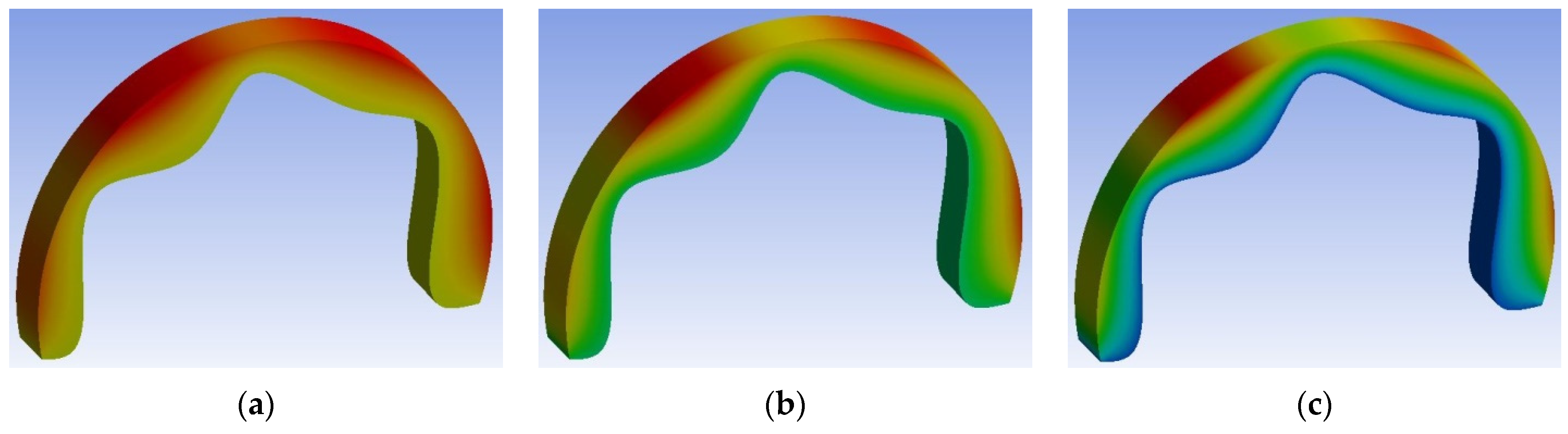
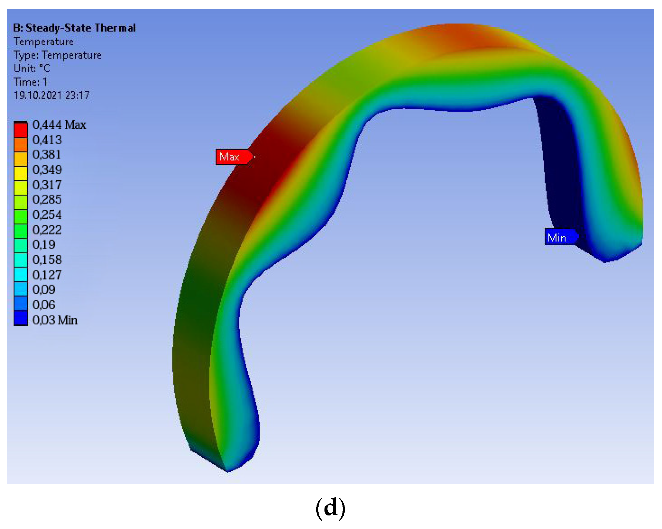
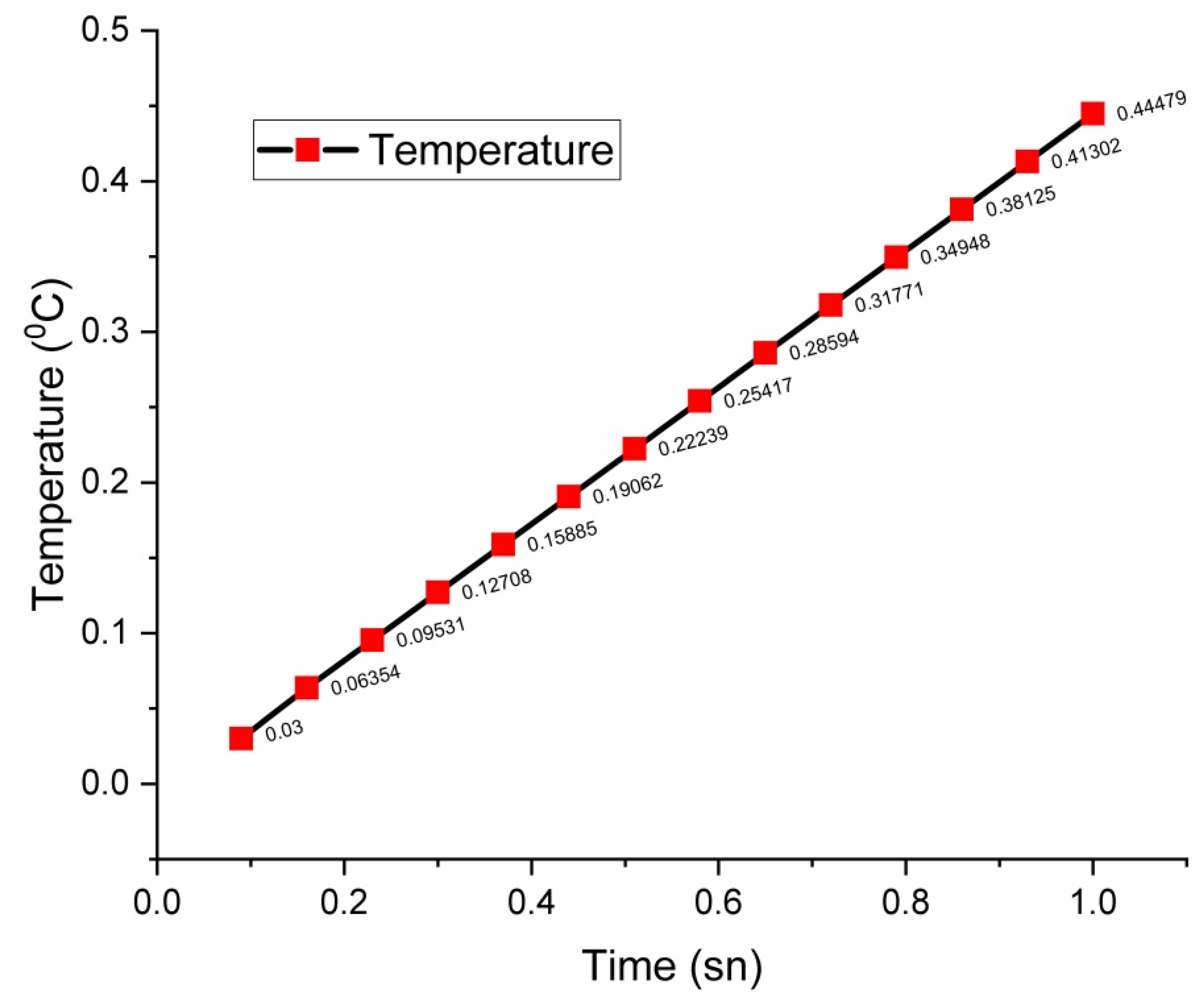
The heat transfer to be applied to the solid model occurs between 1 and 4 s. Performing the simulation for 1 s or longer does not change the heat transfer image. In this study, the play duration of the animation was chosen to be 1 s. The heat transfer distribution after 1 s in different parts of the model is shown in Figure 3. Figure 4 shows the heat transfer distribution images of the model after 4 s. As can be seen from Figure 3; Figure 4, the heat distribution on the solid model surface is similar following different durations. The heat transfer videos of the solid model can be accessed using the Supplementary Materials part. Simulation time does not directly affect surgical practices. However, on the basis of the one-second simulation image, the doctor is able to quickly determine the thickness of the desired area of the skull. This will provide helpful information during surgery. Figure 5 demonstrates the linear change of the heat transfer in the model with respect to time.
It can be observed that heat transfer is directly proportional to the model section thickness. As a result, the measured temperature value increases linearly. Selecting random points on the outer surface of the model, the x-, y-, and z-axis values of these points can be obtained. Thanks to the help of Euclidean distance, the distance between these points on the outer surface of the model and the points on the inner surface can be found. Euclidean distance is computed in n-dimensional space using the following expression:
where and are randomly selected points in 3D space.
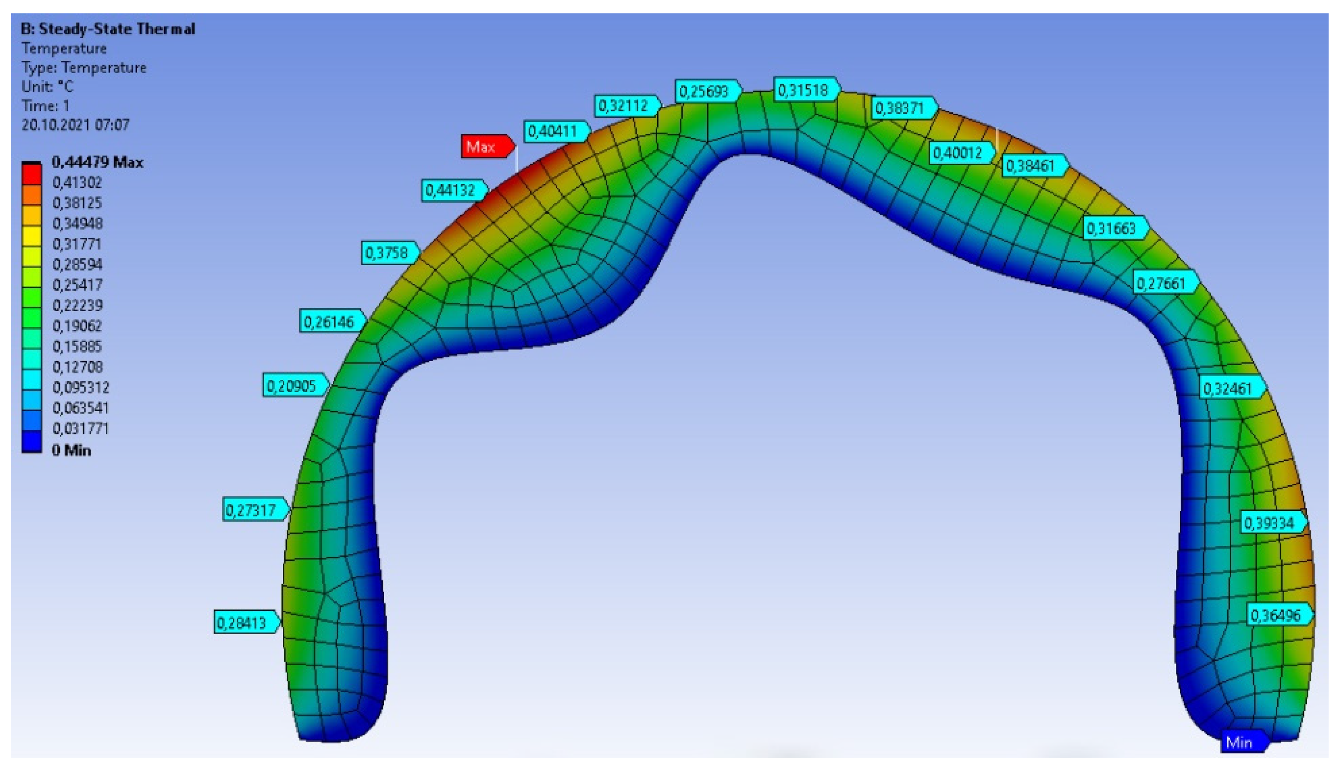
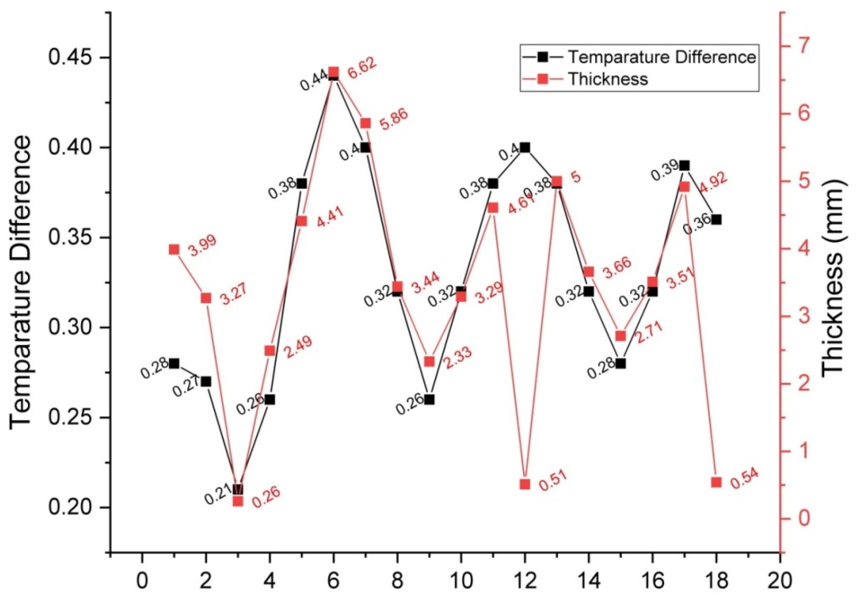
In Figure 6, the temperature values and the highest and lowest values of the points marked on the model are shown. In Figure 7, the distances of the marked points from the inner surface are given. As can be seen from Figure 7, the temperature difference changes in direct proportion to the thickness of the object.
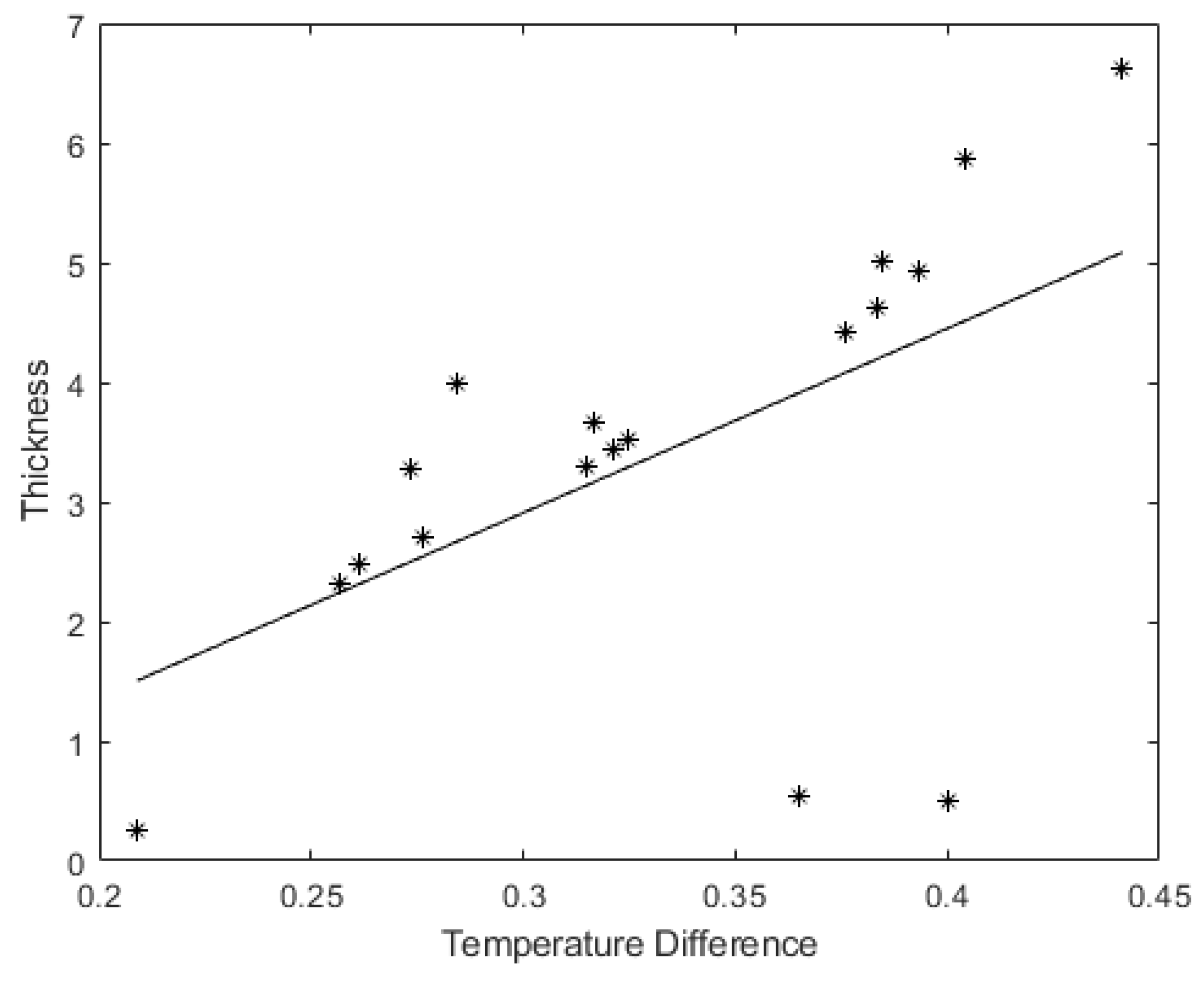
After obtaining the temperature difference dataset at randomly selected points, the least-squares method is applied to find the line that best fits the distribution of the data points. Thus, information on the existence of a relationship between variables is obtained using the least-squares method [38].
Temperature difference is selected as the independent variable, and the distance of the temperature difference from the inner surface is selected as the dependent variable. In this method, for , the line that best fits the data pairs can be determined by using the basis expression . Thickness values corresponding to temperature values are calculated as follows:
Unknown values are estimated by the least-squares method using a random sample from the main population. The data used in this paper consist of the temperature difference at points on the outer surface of the model.
On the basis of the possible values of , the expression can be obtained. Thus, a linear regression model can be drawn using the estimated values. Figure 8 shows the linear regression model between temperature difference and object thickness. Thus, when any point on the outer surface of the designed skull-like model is marked, the thickness value corresponding to the point marked can be found using the least-squares method.
It can be observed that the thermal analysis and finite element methods effectively determine the thickness in all regions of the solid models. In the next section, these methods will be used to determine bone thickness information for human skull images.
2.4. Firat University Neurosurgery Dataset (FUND)
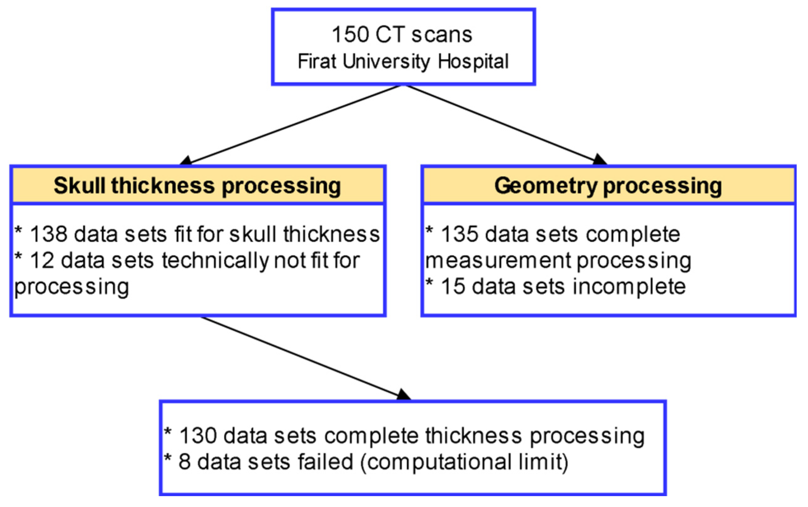
CT data were obtained from the neurosurgery department (Firat University Hospital, Elazığ, Turkey). All CT scans were scanned for any pathological issues. Those with pathological problems were excluded from further analysis. Included were those who did not have visible pathological or unusual morphology. A total of 150 patients were contacted for this study. The age range of the individuals was selected to be 0–72 years. Relevant CT scan data were retrieved from the hospital archive for further processing. The dataset of 150 patients was analyzed, and both 2D and 3D measurements were obtained (Figure 9).
The slice thickness of the CT data ranges from 0.5 to 0.625 mm. Voxel size is isometric, with a 512 × 512-pixel matrix. Voxel size is an important component of CT image quality [39]. A voxel is the 3D analog of a pixel. Voxel size is related to both pixel size and slice thickness. If the pixel size is smaller, the spatial resolution of the image is greater. The CT images of 130 patients used in this study were collected from the same tomography device. Since the Frames, PixelSpaceX, PixelSpaceY, PixelSpaceZ and Slice Thickness values of these patients were similar, not all of them were included in the study. Detailed information on the CT data used in this paper is given in Table 3. In this table, 10 patients were randomly selected from among the total of 130 patients. All skull CT information used in the study can be accessed from the Supplementary Materials part. There is no private information of the patients on this list.
3. Proposed Skull Thickness Analysis Method
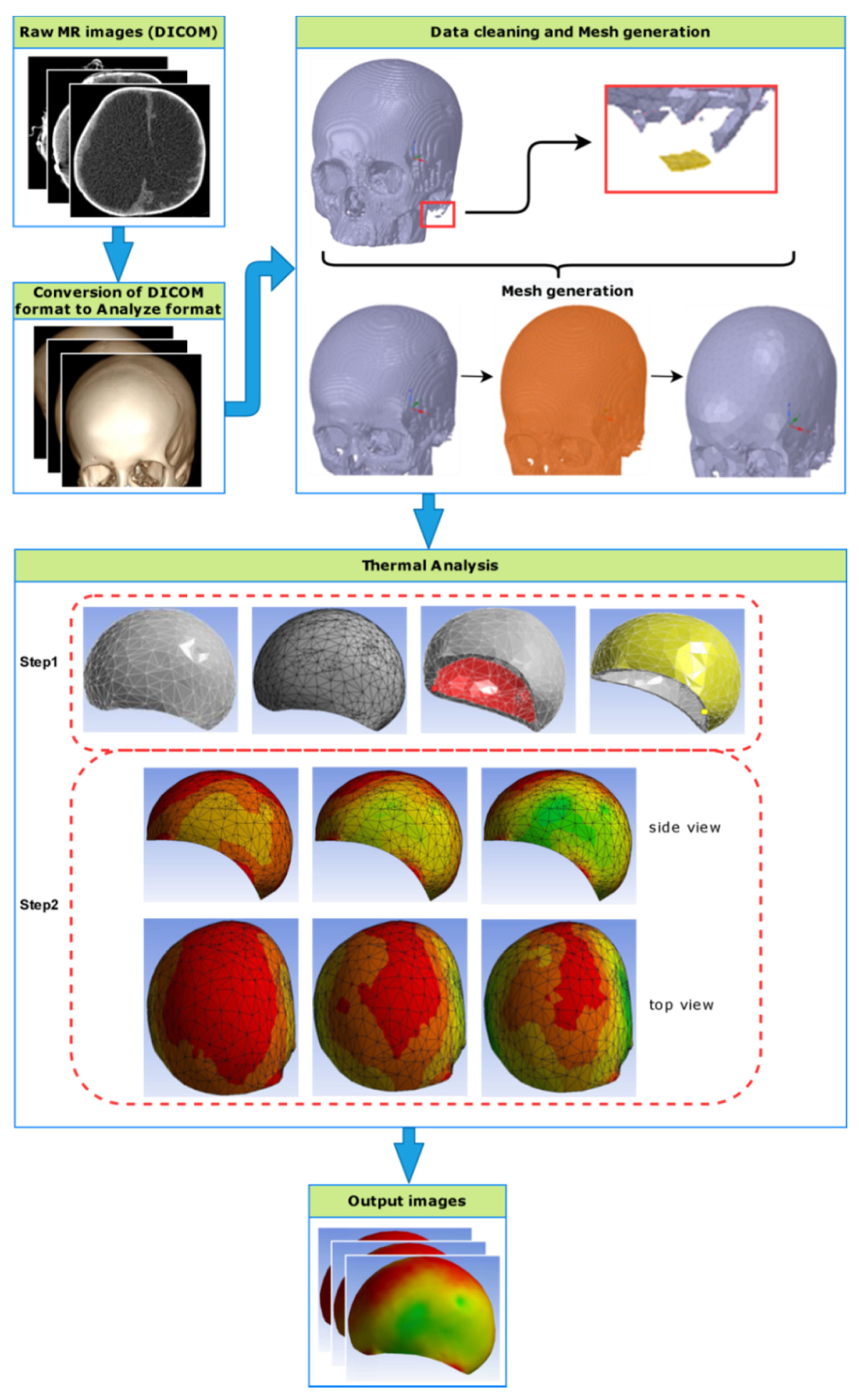
In this study, a new method is developed to calculate bone thickness in all regions of the human skull on the basis of CT images using finite element analysis and thermal analysis methods. Images of skulls from people of different ages and genders were analyzed using CT scans. Analyses were performed with ANSYS [40], which is used in computer-aided engineering studies. Based on the finite element method, the ANSYS Workbench platform allows effective studies in different disciplines, such as mechanics, fluid dynamics, and heat transfer. Additionally, the thermal analysis method based on heat transfer, which is used in various engineering problems, was also used in this study, and the heat transfer was measured with respect to bone thickness. A graphical abstract of the proposed method is given in Figure 10.
The proposed method includes the following main steps:
- 1-
- Raw skull CT images are taken in DICOM format.
- 2-
- DICOM data are transformed into computer-based design models for analysis. In this transformation, the data are recorded in STL file format.
- 3-
- Some undesired bone particle regions obtained from CT should be removed. The STL files are cleared of errors caused by CT scanning in the SpaceClaim software, and these images are thereby made ready for analysis. Thus, the skull image is prepared for the mesh production process. Mesh production is performed using the appropriate number of nodes and elements. Thus, the meshed skull image is suitable for thermal analysis.
- 4-
- In this step, steady-state thermal analysis is carried out. Certain temperature values are applied to the inner and outer surfaces of the skull. In this paper, the internal temperature value is denoted as 0 °C. When the inner surface temperature value is set at 0 °C, the inner–outer temperature difference will automatically be equal to the outer surface temperature value. The temperature values on the outer surface of the skull images are taken along two perpendicular curves.
- 5-
- When obtaining bone thickness using temperature information, the distance between any skull point along the perpendicular curves and the closest inner surface point to this point is used. By using the Euclidean distance between these two points, the bone thickness information of the relevant point can be obtained.
4. Experimental Results
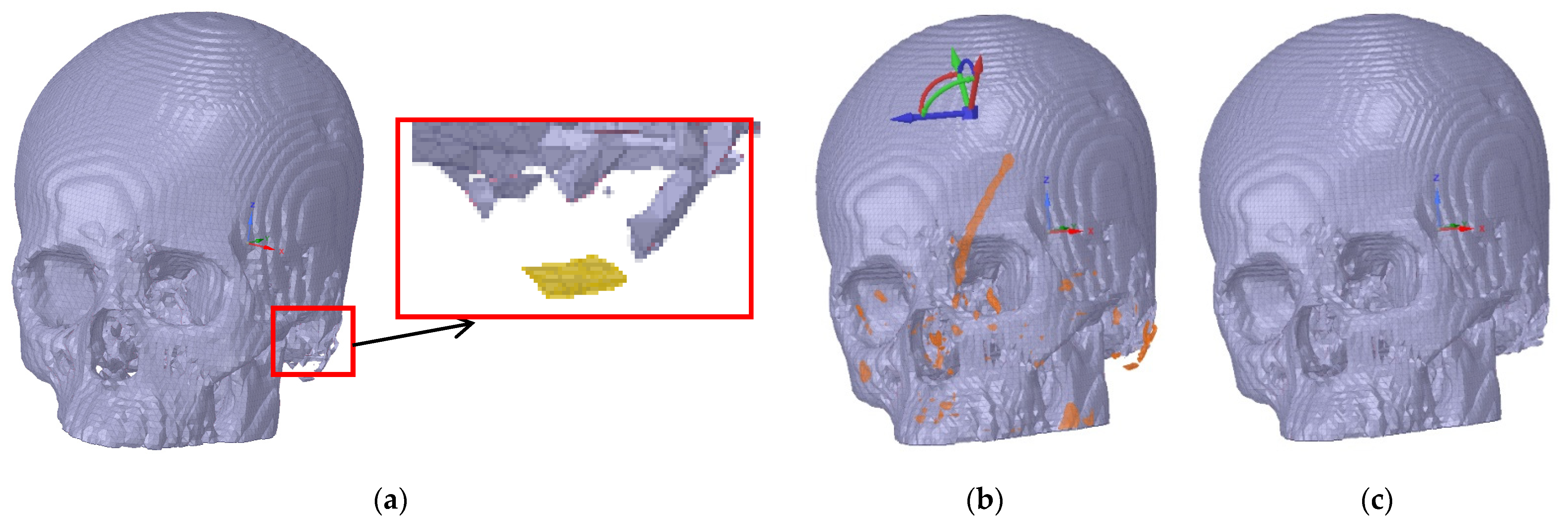
To perform thermal analysis of CT data in the ANSYS program, they must first be defined in SpaceClaim software. These identified data are STL-type files known as “Stereolithography”. STL is a format created by dividing the surfaces of the 3D-designed model into multiple triangles in a mathematical array [41]. This format allows the storage and transmission of the volume information of a 3D skull without any color or texture information. Two-dimensional section images of the human skull are created with the help of computed tomography. These images are overlaid and then made into a 3D model using appropriate software. In this study, RadiAnt DICOM Viewer software is used as the first step to rearrange the surface geometries of skull CT images [42]. CT data is then saved in STL format and meshed using RadiAnt software. When the STL file format is prepared, the number of meshes created on the surface of the skull is directly proportional to the skull’s resolution. STL files prepared in the second step are transferred to SpaceClaim software. Thus, the meshed skull images are analyzed and prepared for ANSYS. Before being taken to ANSYS for thermal analysis, all of the mesh bodies with multiple unconnected regions on the skull surface are separated. The separation of mesh bodies is an important operation for ANSYS analysis. Figure 11 shows an example of unconnected regions on the skull image. All unconnected regions are removed from the skull for a more robust analysis.
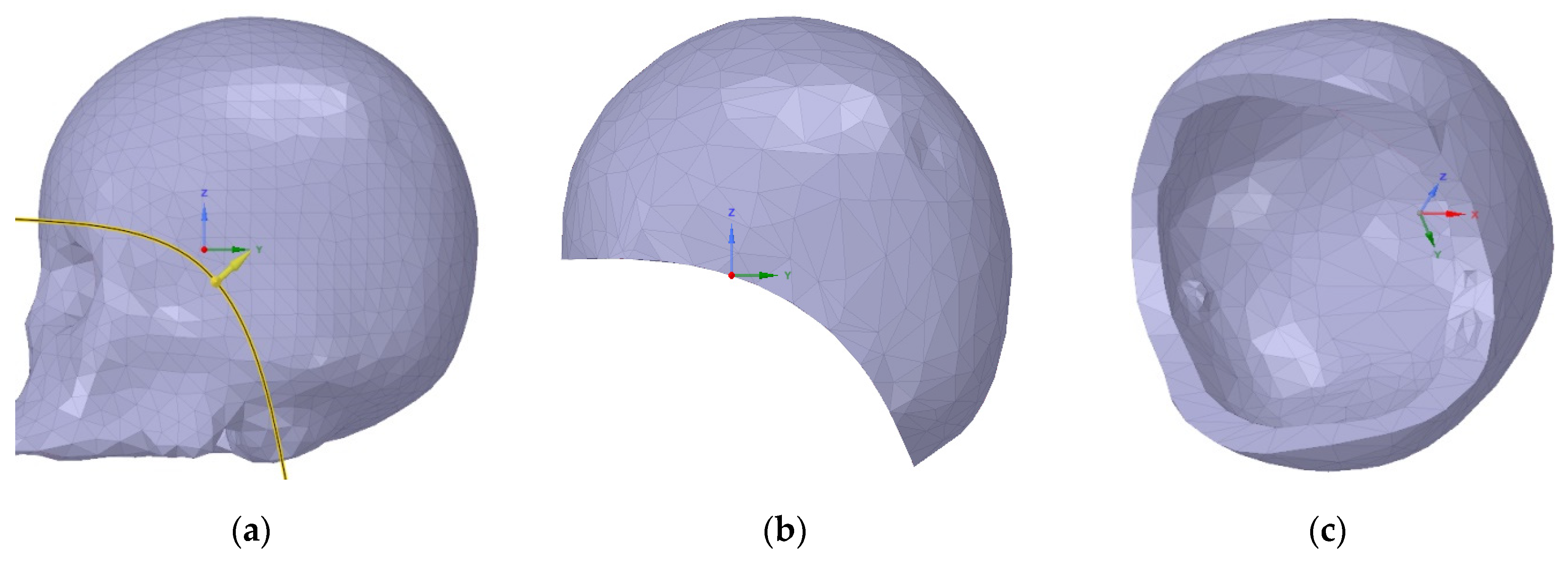
Access to the inner surface is necessary in order to determine the skull’s thickness. Therefore, as seen in Figure 12, the facial region of the skull is removed by drawing a curve from the forehead to the neck. Thus, access to the meshed inner region is provided.
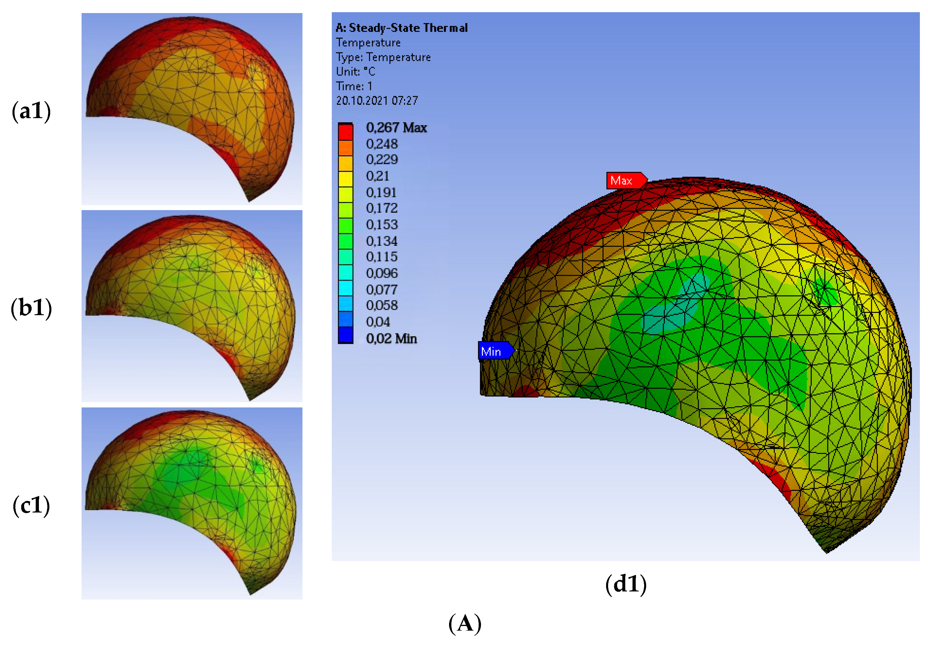
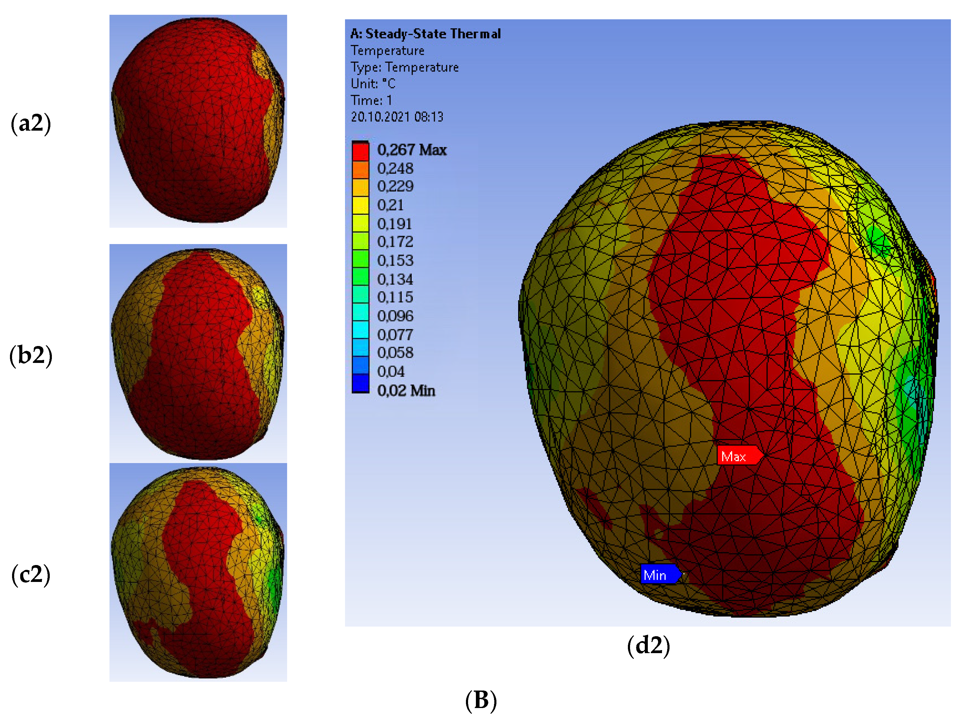
Then thermal analysis is performed using ANSYS Workbench. The temperature value of the skull’s inner surface is assumed to be 0 °C. Thus, the temperature value of any point on the skull’s outer surface gives the temperature difference directly. The heat transfer is performed within one second. There is no difference between simulating for one second or for longer with respect to the heat transfer image. In this study, the play duration for the animation was selected as one second. Simulation time does not directly inform surgical practices. In Figure 13, the left side and top views of the skull are shown. These thermal analysis results were taken in different periods of heat transfer. The color distributions in the thermal images correspond to different bone thicknesses. The red color indicates the region with the greatest bone thickness. The green color indicates the region with the thinnest bone thickness. Other colors show intermediate values of bone thickness in red and green regions. Thanks to the developed method, the bone thickness information of any desired point on the skull can be obtained numerically.
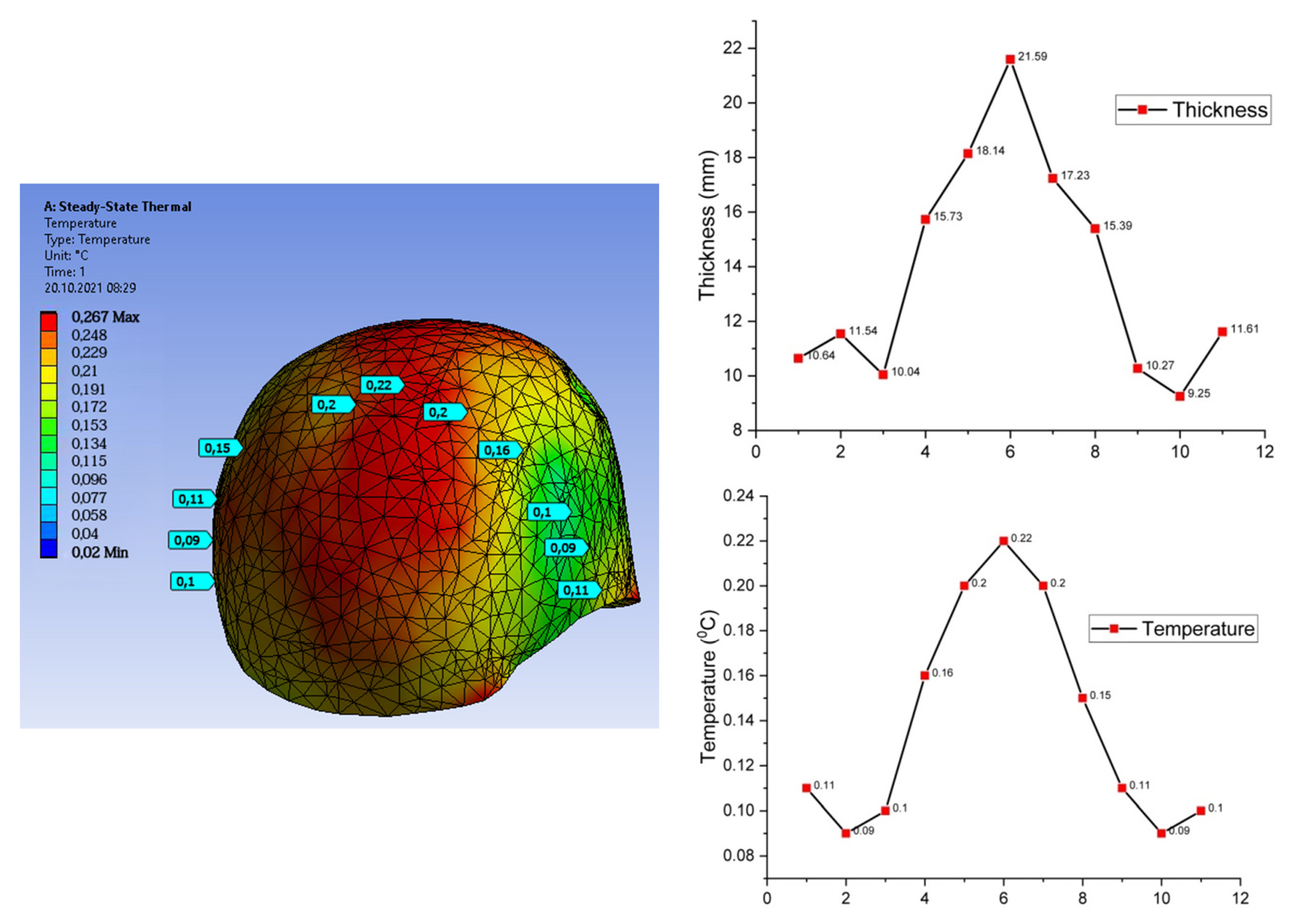
It is well known that the main bone structures in the skull include the frontal, parietal, occipital, and temporal bones. The thickness information at any point of these bones is critical for medical operations. If geometric curves passing over these bones can be found, the thickness information of the desired point can be easily obtained by using the proposed method. Therefore, random points are chosen along two curves that intersect each other as perpendicular axes. The first geometric curve starts from the left temporal bone of the skull, passes over the parietal bone, and ends in the right temporal bone. While the temporal bone forms the sides of the skull, the parietal bone is the bone at which the skull edges and roof join. It was determined on the basis of the temperature differences that the temporal bone is thinner than the parietal bone. This situation is consistent with the related literature [43]. The values of the temperature difference points on the first geometric curve and the distances between the points and the inner surface are shown in Figure 14.
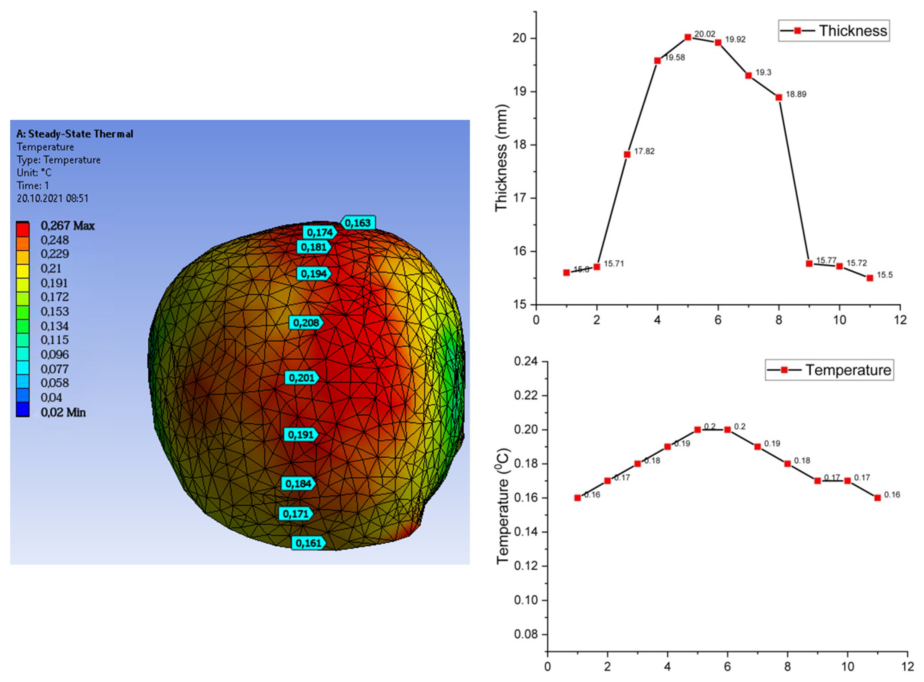
The second geometric curve starts from the frontal bone of the skull and ends at the occipital bone through the parietal bones. While the frontal bone forms the front part of the head, the occipital bone forms the entirety of the posterior part of the skull. The values of the temperature difference points on the second geometric curve and the distances of the points to the inner surface are shown in Figure 15. As mentioned above, the temperature values on the second curve are compatible with the change in the thermal color map. As can be seen from the temperature differences, it was determined that the thickness of the frontal bone and the thickness of the occipital bone are close to each other, and they are consistent with the related literature [43].
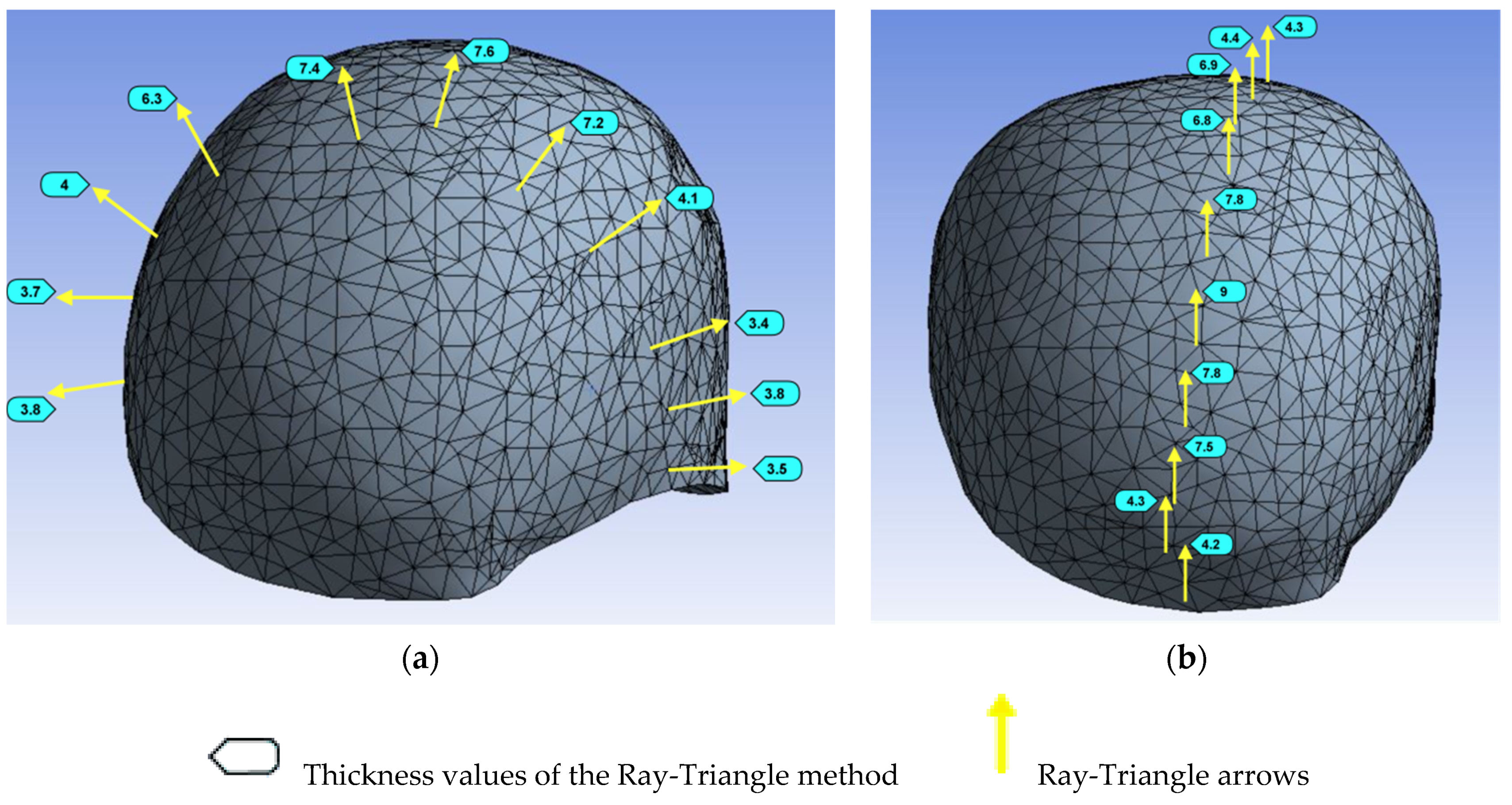
For the purpose of comparison with the proposed method based on thermal analysis, the Ray-Triangle method [44,45], which is able to calculate the thickness in 3D objects, was applied to the manuscript data. Random points were selected along the geometric curve drawn from the frontal bone to the parietal bone and the geometric curve drawn from the left temporal bone to the right temporal bone. First, the coordinate values of the selected points in 3D space were recorded. The Ray-Triangle method was used to pass through these points. The skull thickness values obtained by the Ray-Triangle method are shown in Figure 16. The skull thickness values of the proposed method and the Ray-Triangle method were compared.
Skull thickness measurements of dead people are performed by doctors by piercing the skull with mechanical instruments. However, since this method is not used in living people, doctors perform thickness measurements using special programs such as 3D Slicer. To confirm the reliability of the results obtained, ground truth measurement data are used. The measurement results obtained manually by the doctor are accepted as ground truth. “Ground truth” refers to a set of measurements that are known to be much more accurate than the measurements from the proposed method we are testing. The results of the thermal analysis and Ray-Triangle methods were compared with the ground truth measurement thickness values. The measurement results of the proposed method, the Ray-Triangle methods, and ground truth are shown in Figure 17. As can be seen from the measurement results, the accuracy of the proposed thermal analysis-based method is closer to the ground truth thickness values. A second advantage of the thermal analysis method over the Ray-Triangle method for the measurement of skull thickness is that the entire area of the skull can be measured. With the Ray-Triangle method, only the results of the determined coordinate values can be found.
As seen in Figure 17, the proposed method found the thicknesses to be the same at four points along both curves. The thickness values of other points could be calculated to within an acceptable range. However, it was observed that the Ray-Triangle method was insufficient to measure skull bone thickness values.
5. Conclusions
The goal of this study was to characterize how skull thickness changes with age and sex. Regardless of gender, the general trend of skull thickness increased with age. This increase was greatest in the frontal and parietal bones of the skull. To our knowledge, this is the first study to have calculated 3D skull thickness on the basis of thermal analysis for all age groups. In this study, thermal analysis was performed on the skull CT images of 150 patients (female: 80, 53.3%; male: 70, 46.7%; mean age: 14.3) of different sexes, aged 0–72 years. There was no significant difference in age between men and women patients (female: 14; male: 14.7 mean age). Since the procedure is non-surgical, it can be easily performed in a standard laboratory. Thus, skull thickness measurements were performed on the basis of thermal color maps, and the bone thicknesses were calculated at the desired points. The anatomical complexity of the skull bones was eliminated. Thanks to the developed method, human skull bone thicknesses were calculated on the basis of the thermal analysis and finite element methods, instead of by using invasive techniques.
Experiments on CT skull data illustrated that the proposed thermal analysis-based model is discriminative and powerful for tasks involving the determination of skull bone thickness. The average thicknesses of skull bones for men (frontal: 7.8 mm, parietal: 9.6 mm, occipital: 10.1 mm, temporal: 6 mm) and women (frontal: 8.6 mm, parietal: 10.1 mm, occipital: 10 mm, temporal: 6 mm) was given. The difference (10%) between men and women appears to be statistically significant only for frontal bone thickness. Experimental studies proved that the results obtained using the proposed method were compatible with the related literature. However, the proposed method determined, in accordance with the literature, that the occipital bone was the thickest skull bone and the frontal bone was the second-thickest skull bone. It was also obtained using the proposed method that the temporal bones were the thinnest bones of the skull.
The results obtained in this study offer convenience and speed to doctors when deciding on the material thickness required to join/repair broken bone in the skull. In addition, information will be available to experts when determining distinguishing diagnostic features of bones in skull injuries. Since some color irregularity may occur in skull images, there may be minimal change in the heat transfer of some parts of the skull. Future work will also focus on the color mapping robustness of our approach.
Supplementary Materials
The following are available online at https://0-www-mdpi-com.brum.beds.ac.uk/article/10.3390/app112110483/s1, Table S1: All skull CT data, Video S1: Heat transitions of the model 1 s, Video S2: Heat transitions of the model 4 s.
Author Contributions
Conceptualization, M.C., M.F.T., D.Y.P., K.G.; Methodology, M.C., M.F.T.; Software, M.C., M.F.T.; Manual Measurement, M.C., M.F.T.; Investigation, M.C., M.F.T.; Writing—Review and Editing, M.C., M.F.T., D.Y.P., K.G.; Visualization, M.C., M.F.T.; Supervision, M.F.T.; Funding Acquisition, D.Y.P., K.G. All authors have read and agreed to the published version of the manuscript.
Funding
This research received no external funding.
Institutional Review Board Statement
The study was conducted according to the protocol approved by the Inonu University, Turkey (project code: 2016/16-278). All procedures performed in studies involving human participants were in accordance with the ethical standards of Firat University Hospital Committee and with the 1964 Helsinki declaration or comparable ethical standards.
Informed Consent Statement
Informed consent was obtained from all subjects involved in the study.
Data Availability Statement
The raw/processed data required to reproduce these findings cannot be shared at this time as the data also form part of an ongoing study.
Acknowledgments
The authors would like to thank Sait Ozturk (Firat University, Department of Neurosurgery) for his support and assistance with this study.
Conflicts of Interest
The authors declare no conflict of interest.
Abbreviations
The following abbreviations are used in this manuscript.
| CT | Computed tomography |
| FEM | Finite element method |
| 3D | Three-dimensional |
| DICOM | Digital imaging and communications in medicine |
| STL | Stereolithography |
| FUND | Firat University neurosurgery dataset |
References
- Kung, W.-M.; Tzeng, I.-S.; Lin, M.-S. Three-Dimensional CAD in Skull Reconstruction: A Narrative Review with Focus on Cranioplasty and Its Potential Relevance to Brain Sciences. Appl. Sci. 2020, 10, 1847. [Google Scholar] [CrossRef] [Green Version]
- Flores-Justa, A.; Baldoncini, M.; Pérez Cruz, J.C.; Sánchez Gonzalez, F.; Martínez, O.A.; González-López, P.; Campero, Á. White Matter Topographic Anatomy Applied to Temporal Lobe Surgery. World Neurosurg. 2019, 132, e670–e679. [Google Scholar] [CrossRef] [PubMed]
- Wang, S.-H.; Ko, Y.-C.; Tsai, M.-T.; Fuh, L.-J.; Huang, H.-L.; Shen, Y.-W.; Hsu, J.-T. Can Male Patient’s Age Affect the Cortical Bone Thickness of Jawbone for Dental Implant Placement? A Cohort Study. Int. J. Environ. Res. Public Health 2021, 18, 4284. [Google Scholar] [CrossRef]
- Frank, K.; Gotkin, R.H.; Pavicic, T.; Morozov, S.P.; Gombolevskiy, V.A.; Petraikin, A.V.; Movsisyan, T.V.; Koban, K.C.; Hladik, C.; Cotofana, S. Age and Gender Differences of the Frontal Bone: A Computed Tomographic (CT)-Based Study. Aesthet. Surg. J. 2019, 39, 699–710. [Google Scholar] [CrossRef] [PubMed]
- Tornberg, A.; Jacobsson, L. Care and consequences of traumatic brain injury in Neolithic Sweden: A case study of ante mortem skull trauma and brain injury addressed through the bioarchaeology of care. Int. J. Osteoarchaeol. 2018, 28, 188–198. [Google Scholar] [CrossRef]
- Yellinek, S.; Cohen, A.; Merkin, V.; Shelef, I.; Benifla, M. Clinical significance of skull base fracture in patients after traumatic brain injury. J. Clin. Neurosci. 2016, 25, 111–115. [Google Scholar] [CrossRef]
- Modi, Y.K.; Sanadhya, S. Design and additive manufacturing of patient-specific cranial and pelvic bone implants from computed tomography data. J. Braz. Soc. Mech. Sci. Eng. 2018, 40, 503. [Google Scholar] [CrossRef]
- Lillie, E.M.; Urban, J.E.; Lynch, S.K.; Weaver, A.A.; Stitzel, J.D. Evaluation of Skull Cortical Thickness Changes with Age and Sex from Computed Tomography Scans. J. Bone Miner. Res. 2016, 31, 299–307. [Google Scholar] [CrossRef] [Green Version]
- Kidder, J.H.; Durband, A.C. A re-evaluation of the metric diversity within Homo erectus. J. Hum. Evol. 2004, 46, 297–313. [Google Scholar] [CrossRef]
- Yang, S.; Zhao, Y.; Liao, M.; Zhang, F. An Unsupervised Learning-Based Multi-Organ Registration Method for 3D Abdominal CT Images. Sensors 2021, 21, 6254. [Google Scholar] [CrossRef]
- Ebraheim, N.A.; Liu, J.; Patil, V.; Sanford, C.G.; Crotty, M.J.; Haman, S.P.; Yeasting, R.A. Evaluation of skull thickness and insertion torque at the halo pin insertion areas in the elderly: A cadaveric study. Spine J. 2007, 7, 689–693. [Google Scholar] [CrossRef] [PubMed]
- Imagawa, N.; Inoue, K.; Matsumoto, K.; Omori, M.; Yamamoto, K.; Nakajima, Y.; Kato-Kogoe, N.; Nakano, H.; Le, P.T.M.; Yamaguchi, S.; et al. Histological Evaluation of Porous Additive-Manufacturing Titanium Artificial Bone in Rat Calvarial Bone Defects. Materials 2021, 14, 5360. [Google Scholar] [CrossRef] [PubMed]
- Sommer, H.J.; Eckhardt, R.B.; Shiang, T.Y. Superquadric modeling of cranial and cerebral shape and asymmetry. Am. J. Phys. Anthropol. 2006, 129, 189–195. [Google Scholar] [CrossRef] [PubMed]
- Alexandratou, I.; Patrikelis, P.; Messinis, L.; Alexoudi, A.; Verentzioti, A.; Stefanatou, M.; Nasios, G.; Panagiotopoulos, V.; Gatzonis, S. Long-Term Neuropsychological Outcomes Following Temporal Lobe Epilepsy Surgery: An Update of the Literature. Healthcare 2021, 9, 1156. [Google Scholar] [CrossRef] [PubMed]
- Antonakakis, M.; Schrader, S.; Aydin, Ü.; Khan, A.; Gross, J.; Zervakis, M.; Rampp, S.; Wolters, C.H. Inter-Subject Variability of Skull Conductivity and Thickness in Calibrated Realistic Head Models. Neuroimage 2020, 223, 117353. [Google Scholar] [CrossRef] [PubMed]
- Harvey, L.A.; Close, J.C.T. Traumatic brain injury in older adults: Characteristics, causes and consequences. Injury 2012, 43, 1821–1826. [Google Scholar] [CrossRef]
- Hollensteiner, M.; Fürst, D.; Augat, P.; Schrödl, F.; Esterer, B.; Gabauer, S.; Hunger, S.; Malek, M.; Stephan, D.; Schrempf, A. Characterization of an artificial skull cap for cranio-maxillofacial surgery training. J. Mater. Sci. Mater. Med. 2018, 29, 135. [Google Scholar] [CrossRef] [PubMed] [Green Version]
- Smith, K.; Politte, D.; Reiker, G.; Nolan, T.S.; Hildebolt, C.; Mattson, C.; Tucker, D.; Prior, F.; Turovets, S.; Larson-Prior, L.J. Automated measurement of pediatric cranial bone thickness and density from clinical computed tomography. In Proceedings of the Annual International Conference of the IEEE Engineering in Medicine and Biology Society, EMBS, San Diego, CA, USA, 28 August–1 September 2012; Volume 2012, pp. 4462–4465. [Google Scholar]
- Calderbank, T.; Morgan, B.; Rutty, G.N.; Brough, A. An investigation of juvenile cranial thickness-analysis of skull morphometrics across the complete developmental age range. J. Forensic Radiol. Imaging 2016, 4, 70–75. [Google Scholar] [CrossRef] [Green Version]
- Delye, H.; Clijmans, T.; Mommaerts, M.Y.; Sloten, J.V.; Goffin, J. Creating a normative database of age-specific 3D geometrical data, bone density, and bone thickness of the developing skull: A pilot study. J. Neurosurg. Pediatr. 2015, 16, 687–702. [Google Scholar] [CrossRef] [Green Version]
- Hildebrand, T.; Rüegsegger, P. A new method for the model-independent assessment of thickness in three-dimensional images. J. Microsc. 1997, 185, 67–75. [Google Scholar] [CrossRef]
- Deffieux, T.; Konofagou, E.E. Numerical study of a simple transcranial focused ultrasound system applied to blood-brain barrier opening. IEEE Trans. Ultrason. Ferroelectr. Freq. Control 2010, 57, 2637–2653. [Google Scholar] [CrossRef] [PubMed] [Green Version]
- Lynnerup, N. Cranial thickness in relation to age, sex and general body build in a Danish forensic sample. Forensic Sci. Int. 2001, 117, 45–51. [Google Scholar] [CrossRef]
- Shahzad Masood, M.; Ahmad, A.; Alim Mufti, R. Unconventional Modeling and Stress Analysis of Femur Bone under Different Boundary Condition. Int. J. Sci. Eng. Res. 2013, 4, 293–296. [Google Scholar]
- Coats, B.; Margulies, S.S. Material properties of human infant skull and suture at high rates. J. Neurotrauma 2006, 23, 1222–1232. [Google Scholar] [CrossRef] [PubMed] [Green Version]
- Baumer, T.G.; Passalacqua, N.V.; Powell, B.J.; Newberry, W.N.; Fenton, T.W.; Haut, R.C. Age-dependent fracture characteristics of rigid and compliant surface impacts on the infant skull—A porcine model. J. Forensic Sci. 2010, 55, 993–997. [Google Scholar] [CrossRef]
- Gzik, M.; Wolański, W.; Tejszerska, D.; Gzik-Zroska, B.; Koźlak, M.; Larysz, D.; Mandera, M. Application of 3D modeling and modern visualization technique to neurosurgical trigonocephaly correction in children. IFMBE Proc. 2009, 25, 68–71. [Google Scholar] [CrossRef]
- Ramadan, A.N.; Jing, P.; Zhang, J.; Zohny, H.N.E.-D. Numerical Analysis of Additional Stresses in Railway Track Elements Due to Subgrade Settlement Using FEM Simulation. Appl. Sci. 2021, 11, 8501. [Google Scholar] [CrossRef]
- Giuliano, G.; Polini, W. Strain State in Metal Sheet Axisymmetric Stretching with Variable Initial Thickness: Numerical and Experimental Results. Appl. Sci. 2021, 11, 8265. [Google Scholar] [CrossRef]
- Li, W.; Chen, X.; Wang, H.; Chan, A.H.C.; Cheng, Y. Evaluating the Seismic Capacity of Dry-Joint Masonry Arch Structures via the Combined Finite-Discrete Element Method. Appl. Sci. 2021, 11, 8725. [Google Scholar] [CrossRef]
- Ahmed, M.; Singh, D.; AlQadhi, S.; Alrefae, M.A. Improvement of the Zienkiewicz–Zhu Error Recovery Technique Using a Patch Configuration. Appl. Sci. 2021, 11, 8120. [Google Scholar] [CrossRef]
- Chen, Y.; Pani, M.; Taddei, F.; Mazzà, C.; Li, X.; Viceconti, M. Large-scale finite element analysis of human cancellous bone tissue micro computer tomography data: A convergence study. J. Biomech. Eng. 2014, 136, 101013. [Google Scholar] [CrossRef]
- Tiede, U.; Bomans, M.; Höhne, K.H.; Pommert, A.; Riemer, M.; Schiemann, T.; Schubert, R.; Lierse, W. A computerized three-dimensional atlas of the human skull and brain. AJNR. Am. J. Neuroradiol. 1993, 14, 551–561. [Google Scholar] [CrossRef]
- Semeniuk, B.P.; Göransson, P.; Dazel, O. Dynamic equations of a transversely isotropic, highly porous, fibrous material including oscillatory heat transfer effects. J. Acoust. Soc. Am. 2019, 146, 2540. [Google Scholar] [CrossRef] [PubMed] [Green Version]
- Beckman, W.A. Solar Engineering of Thermal Processes; John Wiley & Sons: Hoboken, NJ, USA, 2013; ISBN 9780470873663. [Google Scholar]
- Webster, J.G. Mechanical Variables Measurement: Solid, Fluid, and Thermal; CRC Press: Boca Raton, FL, USA, 2000. [Google Scholar]
- Sagar, M.V.; Suresh, N. Thermal Analysis of Engine Cylinder with Fins by using ANSYS Workbench. Int. J. Eng. Res. 2017, 6, 502–514. [Google Scholar] [CrossRef]
- Wang, H.Y.; Yang, M.; Stufken, J. Information-Based Optimal Subdata Selection for Big Data Linear Regression. J. Am. Stat. Assoc. 2019, 114, 393–405. [Google Scholar] [CrossRef]
- Shafiq-Ul-Hassan, M.; Zhang, G.G.; Latifi, K.; Ullah, G.; Hunt, D.C.; Balagurunathan, Y.; Abdalah, M.A.; Schabath, M.B.; Goldgof, D.G.; Mackin, D.; et al. Intrinsic dependencies of CT radiomic features on voxel size and number of gray levels. Med. Phys. 2017, 44, 1050–1062. [Google Scholar] [CrossRef]
- Ansys 2020 R1. Available online: https://www.ansys.com/products/release-highlights (accessed on 28 October 2021).
- Grothe, T.; Brockhagen, B.; Storck, J.L. Three-dimensional printing resin on different textile substrates using stereolithography: A proof of concept. J. Eng. Fiber. Fabr. 2020, 15, 1–7. [Google Scholar] [CrossRef]
- RadiAnt DICOM Viewer. Available online: https://www.radiantviewer.com/ (accessed on 28 October 2021).
- Ekşi, M.Ş.; Güdük, M.; Usseli, M.I. Frontal Bone is Thicker in Women and Frontal Sinus is Larger in Men. J. Craniofac. Surg. 2021, 32, 1683–1684. [Google Scholar] [CrossRef] [PubMed]
- Möller, T.; Trumbore, B. Fast, minimum storage ray/triangle intersection. In Proceedings of the ACM SIGGRAPH 2005 Courses SIGGRAPH 2005, Los Angeles, CA, USA, 31 July–4 August 2005. [Google Scholar] [CrossRef]
- Jaroslaw Tuszynski Triangle/Ray Intersection—File Exchange—MATLAB Central. Available online: https://www.mathworks.com/matlabcentral/fileexchange/33073-triangle-ray-intersection (accessed on 22 August 2021).
Figure 1.
Three-dimensional models produced for thermal analysis.

Figure 2.
Images of meshed solid models with different numbers of nodes and elements: (a) mesh model-1, (b) mesh model-2, and (c) mesh model-3.
Figure 2.
Images of meshed solid models with different numbers of nodes and elements: (a) mesh model-1, (b) mesh model-2, and (c) mesh model-3.

Figure 3.
Heat transitions of the model at (a) 0.3 s, (b) 0.6 s, (c) 0.9 s and (d) 1 s.


Figure 4.
Heat transitions of the model at (a) 1 s, (b) 2 s, (c) 3 s and (d) 4 s.

Figure 5.
Temporal change of model heat transfer.

Figure 6.
Randomly marked points.

Figure 7.
Change of temperature difference according to object thickness.

Figure 8.
Temperature difference thickness relationship.

Figure 9.
Flowchart of the CT processing in the study.

Figure 10.
Graphical abstract of the proposed method.

Figure 11.
(a) Unconnected mesh body. (b) All unconnected mesh bodies (orange color). (c) Skull without unconnected mesh body.
Figure 11.
(a) Unconnected mesh body. (b) All unconnected mesh bodies (orange color). (c) Skull without unconnected mesh body.

Figure 12.
(a) Surface separation curve. (b) Removal of the facial region. (c) Internal region of skull surface.
Figure 12.
(a) Surface separation curve. (b) Removal of the facial region. (c) Internal region of skull surface.

Figure 13.
(A) the left side and heat transfer of the skull in (a1) 0.3 s, (b1) 0.6 s, (c1) 0.9 s and (d1) 1 s; (B) the top views and heat transfer of the skull in (a2) 0.3 s, (b2) 0.6 s, (c2) 0.9 s and (d2) 1 s.
Figure 13.
(A) the left side and heat transfer of the skull in (a1) 0.3 s, (b1) 0.6 s, (c1) 0.9 s and (d1) 1 s; (B) the top views and heat transfer of the skull in (a2) 0.3 s, (b2) 0.6 s, (c2) 0.9 s and (d2) 1 s.


Figure 14.
Temperature and thickness values along the temporal and parietal bones (i.e., first curve).
Figure 14.
Temperature and thickness values along the temporal and parietal bones (i.e., first curve).

Figure 15.
Temperature and thickness values along the frontal and occipital bones (i.e., second curve).
Figure 15.
Temperature and thickness values along the frontal and occipital bones (i.e., second curve).

Figure 16.
Skull thickness measurement results of the Ray-Triangle method: (a) values obtained from left temporal bone to right temporal bone; (b) values obtained from frontal bone to parietal bone.
Figure 16.
Skull thickness measurement results of the Ray-Triangle method: (a) values obtained from left temporal bone to right temporal bone; (b) values obtained from frontal bone to parietal bone.

Figure 17.
The proposed method based on thermal analysis, the Ray-Triangle method, and the manual measurement results: (a) skull thickness values obtained from left temporal bone to right temporal bone; (b) skull thickness values obtained from the frontal bone to the parietal bone.
Figure 17.
The proposed method based on thermal analysis, the Ray-Triangle method, and the manual measurement results: (a) skull thickness values obtained from left temporal bone to right temporal bone; (b) skull thickness values obtained from the frontal bone to the parietal bone.


Table 1.
Material properties of skull bones were obtained by different authors.
| Authors | Young’s Modulus (MPa) | Poisson Ratio | References |
|---|---|---|---|
| Coats and Margulies (2006) | 300 | 0.19 | [25] |
| Baumer et al. (2009) | 238 | 0.20 | [26] |
| Gzik et al. (2009) | 380 | 0.22 | [27] |
Table 2.
FE solution information against different mesh models.
| Model No. | Mesh Size (mm) | Node | Elements | Study Time |
|---|---|---|---|---|
| 1 | 1 | 7635 | 1395 | 3 min, 8 s |
| 2 | 2 | 1435 | 213 | 1 min, 17 s |
| 3 | 3 | 637 | 80 | 0 min, 29 s |
Table 3.
Skull CT data.
| Id | Gender | Age | Frames | PixelSpaceX | PixelSpaceY | PixelSpaceZ | Slice Thickness |
|---|---|---|---|---|---|---|---|
| 1 | M | 16.00 | 742 | 0.546 | 0.546 | 0.5 | 0.5 |
| 2 | M | 16.00 | 305 | 0.488281 | 0.488281 | 0.625 | 0.625 |
| 3 | F | 12.00 | 292 | 0.582031 | 0.582031 | 0.625 | 0.625 |
| 4 | M | 14.00 | 766 | 0.546 | 0.546 | 0.5 | 0.625 |
| 5 | F | 15.00 | 769 | 0.546 | 0.546 | 0.5 | 0.5 |
| 6 | F | 16.00 | 303 | 0.492188 | 0.492188 | 0.625 | 0.625 |
| 7 | M | 14.00 | 296 | 0.488281 | 0.488281 | 0.625 | 0.625 |
| 8 | M | 13.00 | 650 | 0.546 | 0.546 | 0.5 | 0.5 |
| 9 | M | 15.00 | 423 | 0.466797 | 0.466797 | 0.5 | 0.625 |
| 10 | F | 11.00 | 288 | 0.488281 | 0.488281 | 0.625 | 0.625 |
All data used in this study can be reached in Supplementary Materials part.
Publisher’s Note: MDPI stays neutral with regard to jurisdictional claims in published maps and institutional affiliations. |
© 2021 by the authors. Licensee MDPI, Basel, Switzerland. This article is an open access article distributed under the terms and conditions of the Creative Commons Attribution (CC BY) license (https://creativecommons.org/licenses/by/4.0/).
Share and Cite
MDPI and ACS Style
Calisan, M.; Talu, M.F.; Pimenov, D.Y.; Giasin, K. Skull Thickness Calculation Using Thermal Analysis and Finite Elements. Appl. Sci. 2021, 11, 10483. https://0-doi-org.brum.beds.ac.uk/10.3390/app112110483
AMA Style
Calisan M, Talu MF, Pimenov DY, Giasin K. Skull Thickness Calculation Using Thermal Analysis and Finite Elements. Applied Sciences. 2021; 11(21):10483. https://0-doi-org.brum.beds.ac.uk/10.3390/app112110483
Chicago/Turabian StyleCalisan, Mucahit, Muhammed Fatih Talu, Danil Yurievich Pimenov, and Khaled Giasin. 2021. "Skull Thickness Calculation Using Thermal Analysis and Finite Elements" Applied Sciences 11, no. 21: 10483. https://0-doi-org.brum.beds.ac.uk/10.3390/app112110483
Note that from the first issue of 2016, this journal uses article numbers instead of page numbers. See further details here.