
Dual Image-Based CNN Ensemble Model for Waste Classification in Reverse Vending Machine


1
Department of Mechanical and Information Engineering, University of Seoul, Seoul 02504, Korea
2
Department of Smart Cities, University of Seoul, Seoul 02504, Korea
*
Author to whom correspondence should be addressed.
Appl. Sci. 2021, 11(22), 11051; https://0-doi-org.brum.beds.ac.uk/10.3390/app112211051
Submission received: 8 October 2021
/
Revised: 15 November 2021
/
Accepted: 19 November 2021
/
Published: 22 November 2021
(This article belongs to the Special Issue Smart Cities in Applied Sciences)
Abstract
:A reverse vending machine motivates citizens to bring recyclable waste by rewarding them, which is a viable solution to increase the recycling rate. Reverse vending machines generally use near-infrared sensors, barcode sensors, or cameras to classify recycling resources. However, sensor-based reverse vending machines suffer from a high configuration cost and the limited scope of target objects, and conventional single image-based reverse vending machines usually make erroneous predictions about intentional fraud objects. This paper proposes a dual image-based convolutional neural network ensemble model to address these problems. For this purpose, we first created a prototype reverse vending machine and constructed an image dataset containing two cross-sections of objects, top and front view. Then, we chose convolutional neural network models widely used in image classification as the candidates for building an accurate and lightweight ensemble model. Considering the size and classification performance of candidates, we constructed the best-fit ensemble combination and evaluated its classification performance. The final ensemble model showed a classification accuracy higher than 95% for all target classes, including fraud objects. This result proves that our approach achieves better robustness against intentional fraud objects than single image-based models and thus can broaden the scope for target resources. The measurement results on lightweight embedded platforms also demonstrated that our model provides a short inference time that is enough to facilitate the real-time execution of reverse vending machines based on low-cost edge artificial intelligence devices.
1. Introduction
General waste recycling methods can be classified into curbside recycling and paid recycling [1]. Curbside recycling is a simple way to collect recyclable waste, but it cannot reward recycling with payment. On the other hand, reverse vending machine (RVM) [2] is a famous paid recycling method in Europe and the United States, which returns payment for people who recycle resources such as polyethylene terephthalate (PET) bottles or aluminum cans. This direct compensation for recycling can increase the recycling rate. Based on this advantage, studies on introducing RVM for the smooth collection of recycling resources have been conducted [3,4,5].
RVM can also be adopted in smart and sustainable cities for waste management. One of the core elements for waste management in smart and sustainable cities is an on-time collection system with intelligent sensor-based infrastructure and the classification of waste [6]. To meet this goal, studies suggested and surveyed waste management with cloud or Internet of Things (IoT) based systems [7,8]. By this time, RVM has been a successful solution for waste management in many regions [9], and the system is often configured with the embedded platform. Therefore, RVM can be further developed into a system suitable for smart and sustainable cities by applying more accurate image-based classification and IoT with a cloud-based system.
The essential requirements for the RVM system are the accurate and rapid classification of input resources and detection of fraud objects that intend to fool recognition systems [10,11]. The RVM systems currently employ various sensors such as barcode sensors, weight sensors, or near-infrared sensors to satisfy these requirements. The barcode sensor-based RVM system requires binary encoding information of the input resources and its vast up-to-date database. Since barcode sensors can only classify the resources with readable binary encoding information, a system based on barcodes may limit the scope of the target resources. The use of a near-infrared sensor enhances the detection rate. However, it leads to high configuration costs of the RVM system, which may impede the active installation and enhanced accessibility of RVM.
Convolutional neural network (CNN) is one of the most commonly applied techniques for computer vision. It can broaden the scope of the input resources for the RVM system with the dataset consisting of various objects. Furthermore, CNN can decrease the configuration cost of the RVM system because the vision-based RVM system only requires the camera to classify input resources. Therefore, many studies have been conducted to apply CNNs for the RVM system. For example, Kokoulin et al. [12], Kokoulin and Kiryanov [13] compared the performance of single image-based systems with multiple CNNs to classify input objects. Park et al. [14] showed that a single image-based system cannot accurately identify intended fraud objects and proposed a multi-modal network that uses various modalities such as image, weight, and ultrasound. Although this multi-modal network system is robust against fraud objects, the cost incurred in the modality measurement and integration is high.
In summary, the challenges of the current RVM are the limited scope of input resources, high system configuration cost, and inaccurate classification of intentional fraud objects. To come up with these challenges, we propose a dual image-based CNN ensemble model suitable for a lightweight embedded artificial intelligence (AI) platform. The main contributions of our work are as follows:
- We constructed an open access dataset for RVM with three classes by building the prototype RVM and collecting the recycling resources. Since it is challenging to find an adequate open access dataset for RVM, our open access dataset can be one of the baselines for future RVM studies;
- We also analyzed a limitation of conventional single image-based systems that inaccurately classify fraud objects through extensive experiments. Then, we proved that the limitation can be effectively overcome by introducing a CNN ensemble model based on both top and front views of objects;
- Finally, we demonstrated that our proposed model provides short inference time enough to facilitate the real-time execution of RVM built on top of low-cost edge AI devices.
2. Related Work
RVM and CNN: Various studies have been conducted to solve the limited scope of target resources and the high configuration cost of the RVM system, focusing on classification accuracy, speed, and fraud detection rate. For example, Liukkonen [10] showed that it is possible to process an average of 40.8 objects per minute just using six Raspberry Pi cameras. Although it solved the problem of the high cost of the RVM system, it could not solve the limited scope of collection resources since it is a barcode-based system. Sinaga and Irawan [15] and Rahim and Khatib [16] also presented sensor-based low-cost RVMs, but they were also constrained by the limited scope of collection resources and the lack of various test cases. These studies indicate that there should be different modalities besides barcodes to broaden the scope of the target objects in the RVM system.
In the past decades, with high-performance hardware, such as graphics processing units (GPUs), CNNs have shown groundbreaking results in computer vision, speech processing, or face recognition [17]. The two basic building blocks of CNN are the convolutional layer and the pooling layer. Since the convolutional layer generates an output feature map from the input image by the convolution operation of the convolutional filter, called kernel, it can extract the feature of the input image including spatial information. The pooling layer reduces the size of the feature map by subsampling the input data. This two-fold approach enables the extraction of the spatial-independent global feature of input images [18]. Moreover, since the convolutional layer only needs parameters from a convolutional filter, the number of parameters used in the convolutional layer is significantly less than those in a fully connected layer [19]. For this reason, many studies employed CNNs for the RVM system to widen the scope of the target resources.
Kokoulin et al. [12], Kokoulin and Kiryanov [13] introduced an image-based object classification system for PET and aluminum cans. They compared various CNN models such as LeNet, AlexNet, and SqueezeNet, and showed that the best results are derived when LeNet classifies an object into two classes, PET bottles and cans. However, this study is very limited in that it deals with only 15 test cases. Park et al. [14] proposed a multi-modal network to solve the problem that the single image-based RVM system has difficulty in detecting intentional fraud objects. The modalities used in the study are the image, the weight, and the reflected ultrasound of the object, and they applied the attention module and correspondence learning to the model. The result showed that the model accurately classified the target objects, such as plastic bottles, cans, glasses, and non-target fraud objects. However, since the system integrates modality data with a high-cost controller, the system configuration cost is so high that it may not be an alternative for current RVMs.
Neural Network Ensemble: The neural network ensemble technique combines neural networks trained for the same purpose [20]. Typical ensemble methods include bootstrap aggregating (bagging) [21], boosting [22], and stacking [23]. These methods can derive a better performance by integrating the predictions of weak classifiers. Ensemble networks can also achieve better results when each network is trained from different datasets and merged [24]. However, integrating every trained classifier does not always produce optimal results [25], and thus we need to choose the classifiers that fit the application.
The neural network ensemble is being used in various fields such as image classification and detection to improve performance and make a robust model [26,27,28,29]. Chen et al. [26] classified a channel randomly selected for hyperspectral images and then ensembled each classifier with the majority voting to derive the final result. Antipov et al. [27] presented a CNN ensemble model that predicts gender from the face image. This model showed a state-of-the-art performance even using a 10× smaller dataset than previous studies. Manzo and Pellino [28] proposed a neural network ensemble model to diagnose COVID-19 disease from computer tomography images. They demonstrated that combining multiple models produces better results than using a single model. The CNN ensemble technique can also be applied to waste classification. Zheng and Gu [29] proposed a CNN-based model for classifying household solid waste through images by integrating GoogLeNet, ResNet-50, and MobileNetV2. Each model creates three predictive vectors, and the model integrates them using the unequal precision weighting method to derive the final result.
Edge AI Device: As the data from the IoT devices are becoming more complex, it also becomes crucial to extract valuable features from raw sensor data through deep learning. The centralized cloud server generally processes the data obtained from IoT devices. However, processing the huge and complex data in the cloud server can be inefficient since transmission bandwidth between the IoT devices and the cloud server is limited. Edge computing is a useful technology to solve this problem, which decentralizes computing tasks from the cloud server to the edge devices that lie in the IoT gateway layer near the user end [30,31]. Furthermore, it enables using a deep learning model from the edges, and thus only processed data are transferred to the cloud server.
There are various edge AI devices for deep learning inference, including Raspberry Pi, ASUS Tinkerboard, NVIDIA Jetson series, and Google Coral Dev Board [32,33,34]. NVIDIA’s Jetson is the most widely used edge AI device for deep learning tasks among these platforms. Jetson has CPU-GPU heterogeneous architecture, and this architecture provides the CUDA-programmable feature, which leads to acceleration in machine learning [35]. There are multiple devices in the NVIDIA Jetson family, including Jetson Nano, TX1, TX2, and Xavier NX. Ullah and Kim [36] compared the inference time, memory usage, and power consumption of Jetson Nano, TX1, and Xavier NX platforms. Koubaa et al. [37] compared inference time, GPU memory consumption, and detection performance of Jetson Nano, TX2, Xavier NX, and Xavier AGX for face recognition.
3. Materials and Methods
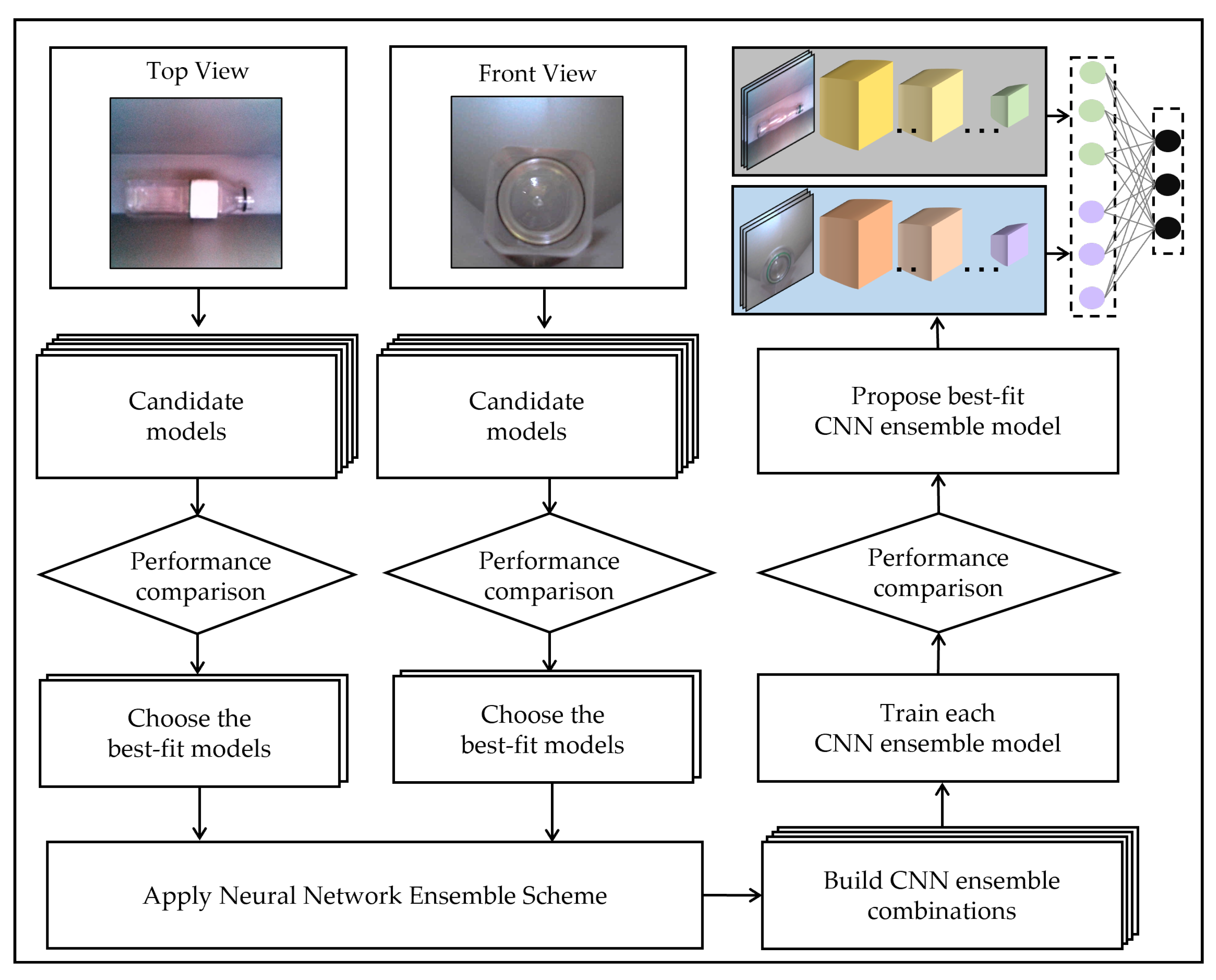
In this section, we suggest a CNN ensemble model for dual image-based and cost-effective RVM. Figure 1 shows the workflow of our study. As the first step, we construct a dual image dataset in our prototype RVM. The images are acquired from top and front views. Next, we choose candidate CNNs from popular image classification models based on their size. Then, we train the candidate CNNs for each view with our dataset and compare both the accuracy and the number of parameters to obtain the best-fit models.
Once the best-fit models from each view are ensembled, we compare the performance of the ensemble models. Finally, we evaluate the inference time of our best ensemble model in lightweight embedded platforms.
3.1. Dataset
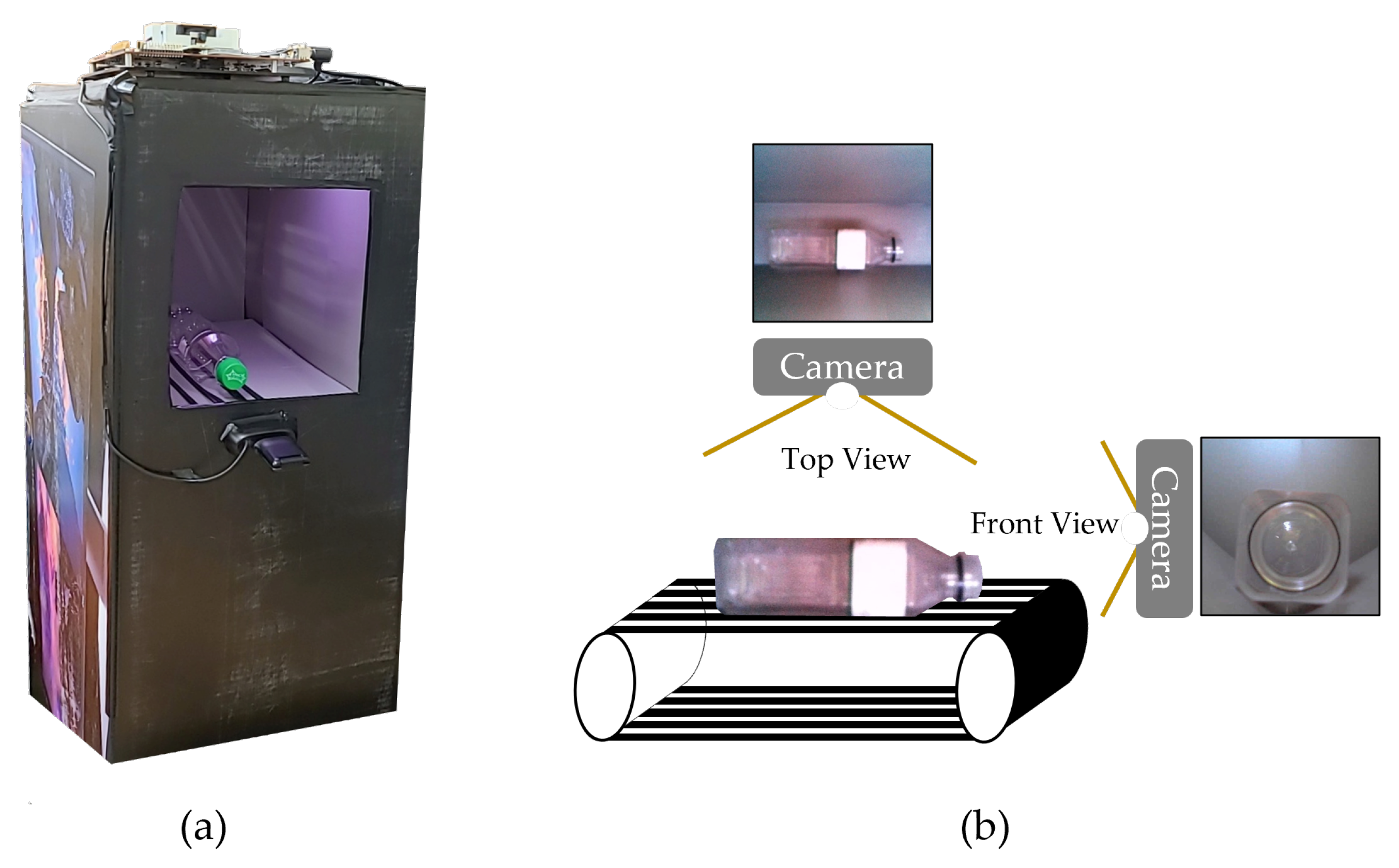
This study constructed the dual image dataset of waste objects by putting the collected resources and capturing their images in the prototype RVM, as shown in Figure 2. We generated two different image samples for each object, that is, a top view and a front view. The resolutions of webcams used for the top view and the front view are 2592 × 1944 and 1280 × 720, respectively. In total, there are 3084 images in our dataset, which are accessible in [38].
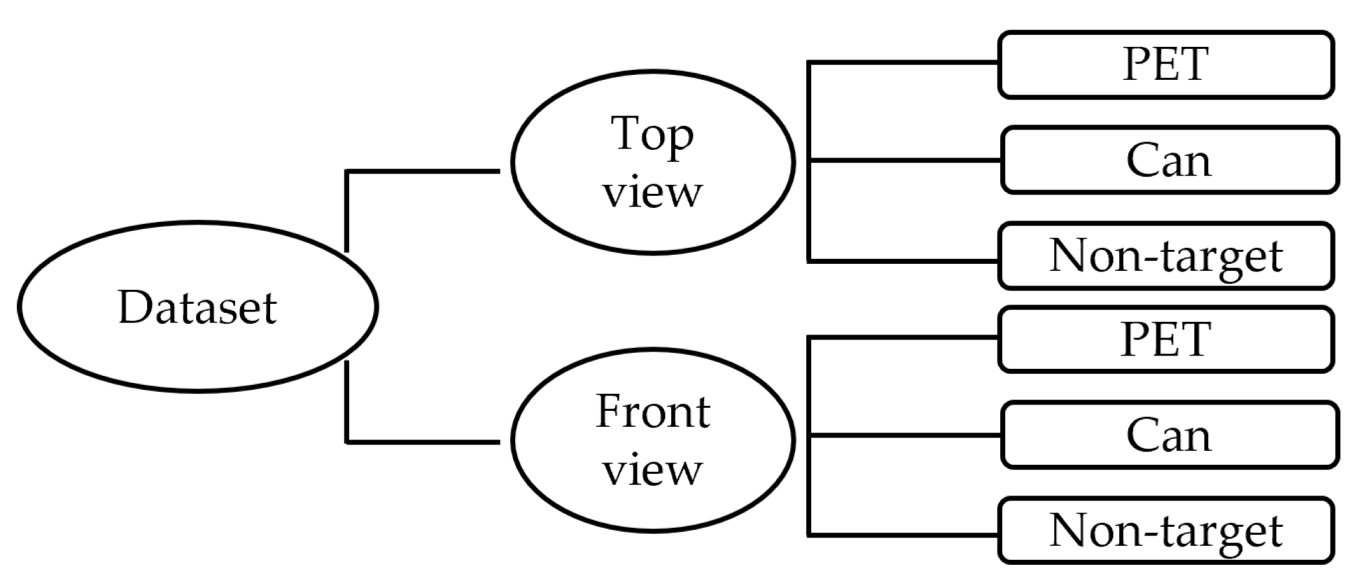
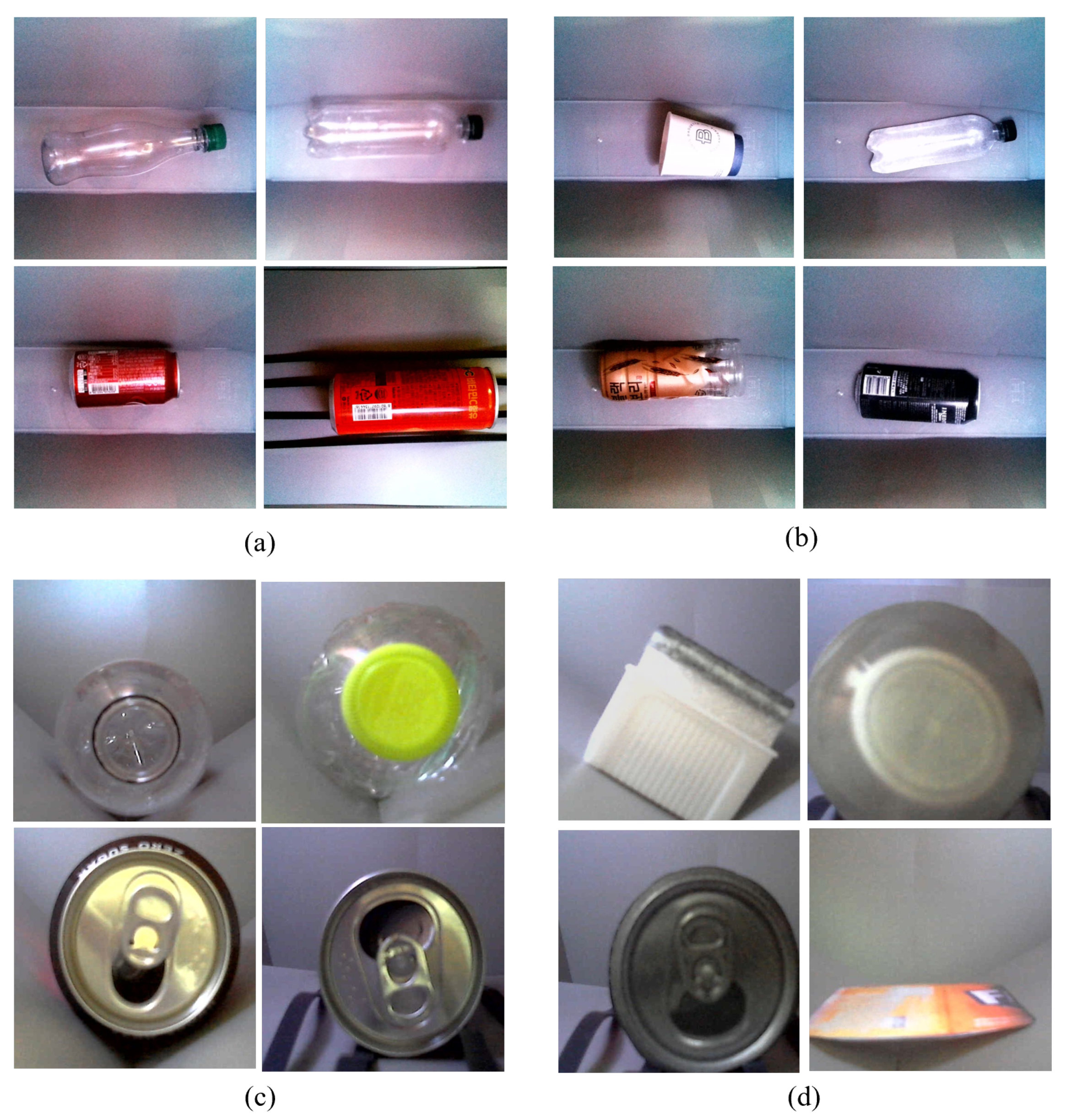
As illustrated in Figure 3, our dataset consists of the top view and the front view images subsets. We further divided each subset into PET, Can, and Non-target classes, which are the most common classification classes of the commercial RVMs [39,40] and the previous studies in [12,13]. The objects belonging to each class are summarized in Table 1. Figure 4 presents actual data samples constructed for our study.
Again, we classify the non-target class objects into fraud objects and inappropriate objects (IAOs). Fraud objects intend to fool the system. They consist of the objects made by printed images of plastic bottles or cans and the objects made only with the label of a plastic bottle. We define the IAOs as general objects inserted carelessly into the RVM, such as roll paper, paper boxes, and even human hands. Even though fraud objects are included in the Non-target class, we used no fraud objects in the training phase and only used IAOs since evaluating untrained fraud objects is one of our intentions. In the test phase, we used the Non-target class dataset consisting of fraud objects and untrained IAOs. More details about detecting fraud objects are presented in Section 3.3 and Section 4.
3.2. Candidate CNN Models
Ensemble model-based classification generally achieves better accuracy but takes a longer processing time. Therefore, the size of the classifier is crucial when building a lightweight model for the embedded AI platform suggested in our study. For this reason, we chose the candidate CNNs among the popular models used in image classification, considering the number of parameters representing the model size. The candidate models addressed in this study are ResNet-50, DenseNet, SquezeNet, MobileNetV2, and EfficientNet-B0/B1/B2.
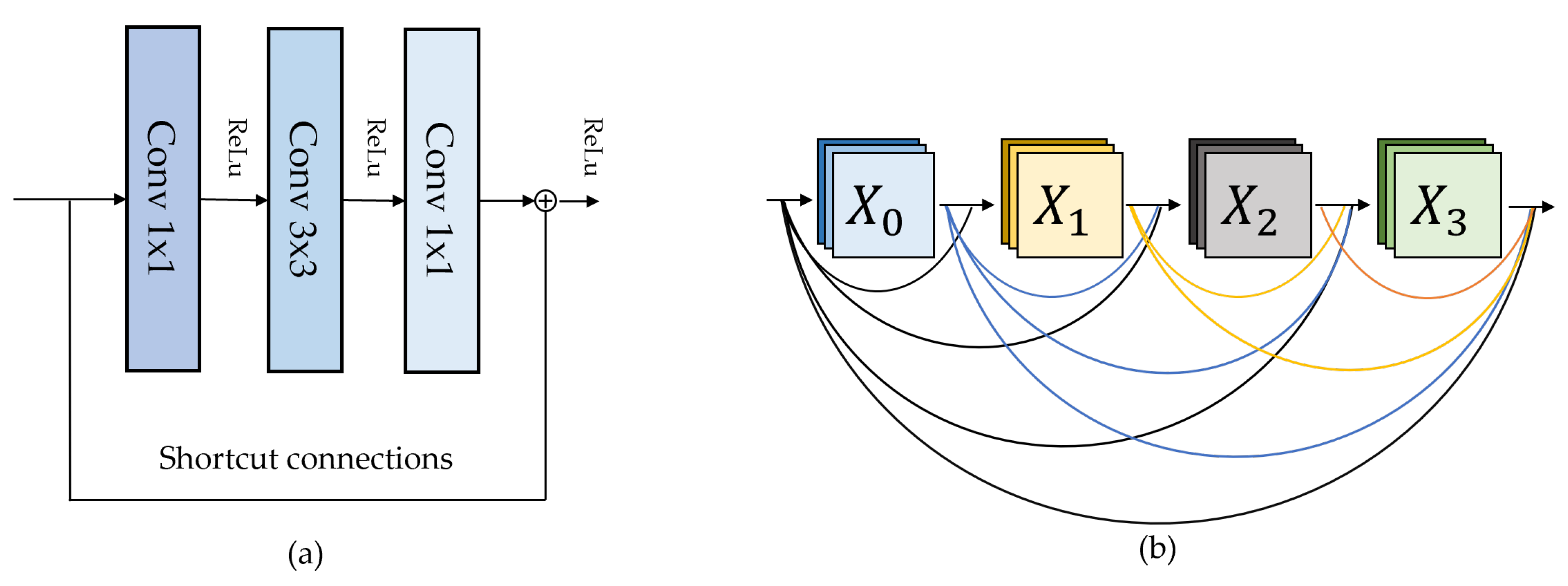
Training deep and complex models is difficult due to the vanishing gradient. Residual neural network (ResNet) [41] and Dense Convolutional Network (DenseNet) [42] are the efficient deep CNNs for addressing the vanishing gradient problem. As shown in Figure 5, ResNet and DenseNet rely on the heaped residual blocks and the stacked dense block, respectively. In addition, both models use shortcut connections to strengthen the gradients. The difference is that ResNet and DenseNet use element-wise addition and concatenation for a shortcut connection, respectively.
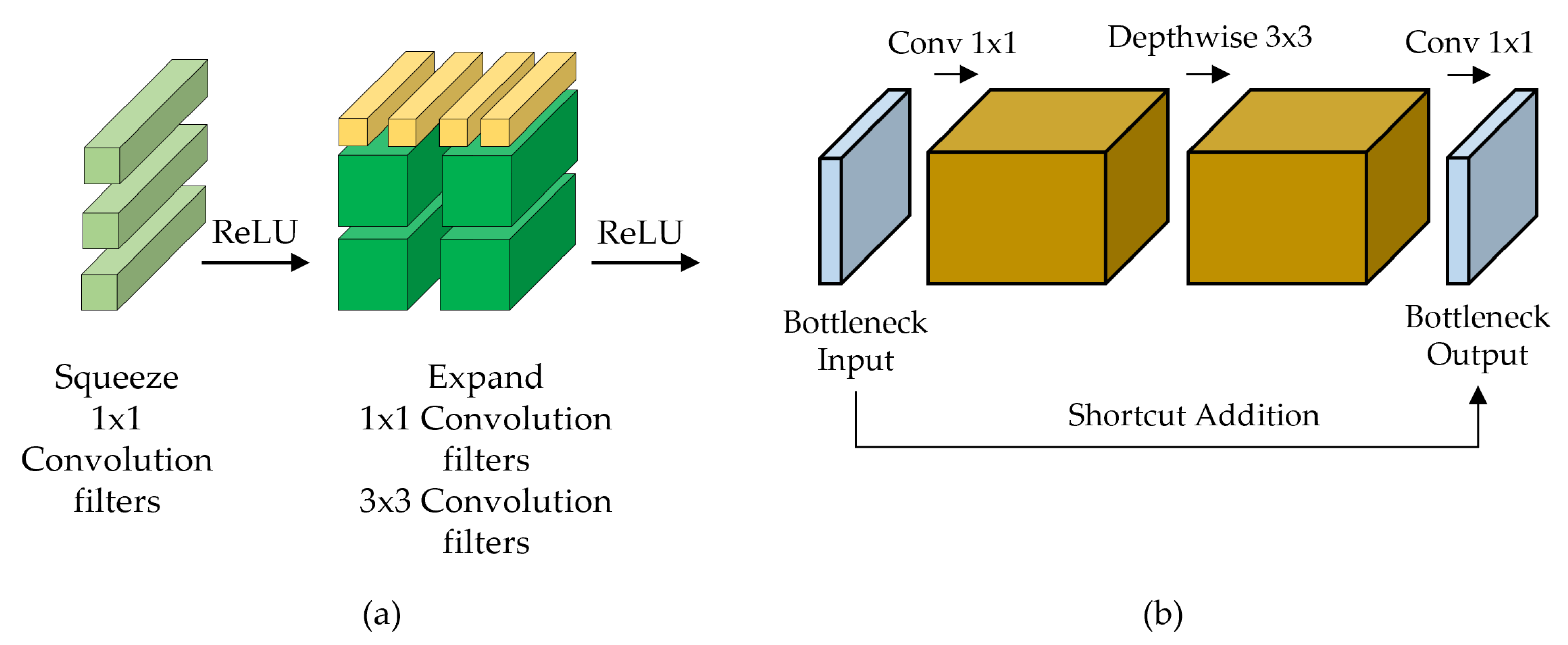
Although embedded devices have very limited computing resources, they need to achieve similar accuracy to conventional models, so lightweight and efficient deep learning models should be used. SqueezeNet [43] and MobileNetV2 [44] are widely used lightweight models for embedded or mobile environments. Figure 6 shows the core modules of SqueezeNet and MobileNetV2. As illustrated in Figure 6a, SqueezeNet [43] consists of the network based on the Fire module that reduces the overall model size. The number of parameters is reduced by 50× compared to AlexNet, but the accuracy on ImageNet has similar or better results. MobileNetV2 [44] aimed to operate real-time in resource-constrained environments where heavy CNN models cannot be used due to weak computational powers. MobileNetV2 uses an inverted residual block and a linear bottleneck to the depthwise separable convolution [45], shown in Figure 6b. The inverted residual block uses a narrow-wide-narrow structure to reduce memory consumption. MobileNetV2 gives similar or better results with fewer parameters and faster inference speed than NasNet-A and ShuffleNet on ImageNet.
Modifying the resolution, depth, or width of CNNs is widely used for enhancing the performance of CNNs. One of the main issues is to decide an adequate factor and its degree for better performance after scaling up. However, this process requires trial and error that causes inefficiency and often results in sub-optimal performance. To overcome such handcrafting, EfficientNet [46] proposed compound scaling, which is a principled way to scale up the model for better performance and efficiency. Compound scaling uniformly scales the three dimensions of depth, width, and resolution with a constant ratio. The experimental result showed that the EfficientNet-B3 achieved better Top-1 accuracy than ResNeXt-101 with 18× fewer FLOPS.
3.3. The Proposed CNN Ensemble Model
We propose an ensemble CNN model using the top and front view images to resolve the limitations of previous state-of-the-art RVM studies using a single image-based system [12,13] or multi-modal network [14]. The main goal of our ensemble approach is to classify fraud objects with high accuracy on a vision-only system.
When building an ensemble network, we can use two strategies: picking the models randomly or using the models with a better performance. Perez et al. [47] suggested that both methods show good results, but in small ensembles the same as in our study, the latter approach can derive a better result. Based on this research, we combine the best-fit CNN models from each view with an ensemble scheme.
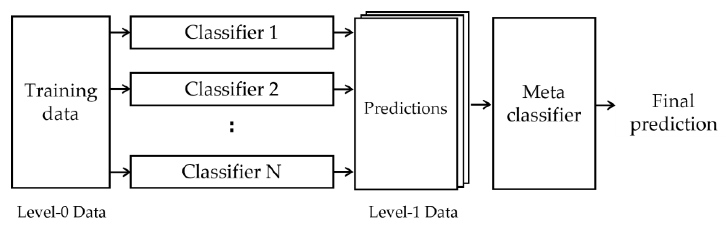
As mentioned in Section 2, typical neural network ensemble techniques are bagging [21], boosting [22], and stacking [23]. All these methods attempt to improve performance by combining weak classifiers to derive robust results. Bagging creates sub-datasets through bootstrap from the original dataset and trains the classifier with the sub-datasets. After the training, the weights for each classifier are set equally, and methods including majority voting produce the final result. Boosting trains the classifiers with the original dataset, and each classifier is weighted differently according to the classifier’s prediction result. After this, the final result is derived from weighted voting or weighted average [48,49]. Stacking or stacked generalization [23] derives the final result through two processes, as illustrated in Figure 7. In the first phase, each classifier is trained with the Level-0 dataset and creates predictions. Then, these predictions become the Level-1 dataset for the meta classifier, and the meta classifier finds the optimal combination of predictions after training. In other words, the meta classifier combines the results obtained by several poor classifiers and derives a robust final result.
General neural network ensemble schemes train each classifier with the same dataset or multiple partial datasets derived from the original dataset. By contrast, we train each classifier on different training sets, that is, a top view and a front view dataset. So, each prediction contains information from a different view. The CNN ensemble model is a small ensemble with two classifiers, and the size of the prediction vectors for each classifier is three. Therefore, we decided that the optimal combination of each classifier with the stacking ensemble scheme fits better than the voting or weighted averaging method in boosting or bagging.
We used the single-layer perceptron (SLP) as the meta classifier in our model to combine two classifiers independently trained from the top view and the front view. Since the SLP is a lightweight and straightforward network, the proposed model can operate in a lightweight embedded platform without any performance problems.
In the proposed stacking ensemble scheme, datasets for SLP are concatenated vectors of the top view and the front view prediction. Using the class probabilities rather than a single class value is recommended since the probabilities represent the confidence measure for the prediction [50,51]. The final result vector derived through the trained SLP goes through the softmax layer and becomes the final prediction vector.
Since RVM is a system that rewards users, it is essential to collect many target objects and reliably identify them simultaneously. Therefore, we do not select the argmax class that has the highest probability from the final prediction vector. Instead, when the probability of the argmax class shows the value above the decision threshold, we select that class as the final class. If it does not exceed the decision threshold, non-target classes are chosen. The decision threshold is an implicit classification metric for non-target objects when the prediction vector does not include the Non-target class. On the other hand, the decision threshold can act as the second verification when the prediction vector includes the Non-target class. For example, suppose that the final prediction vector is given as:
the argmax class indicates that the object is likely to be PET even though the probability of the Non-target class is as high as the PET class. However, with the decision threshold of 0.5, this object is predicted as a non-target class in the end.
The ensemble process of the top view and front view classifier can be expressed as:
where is the final vector and is the j-th element of vector z. is the weight of SLP in our model, connecting i-th element of the input vector to j-th element of the output vector. b is the bias, and is the input vector, after concatenating the result vector of each classifier. N is the size of vector and C is the size of the final vector z, respectively. The final vector z passes the softmax layer , and we can get the class with the highest accuracy. The class with the highest probability H and its probability are defined as:
Finally, we check if the predicted probability is higher than the decision threshold. If it exceeds the threshold, the final result y is H. Otherwise, it becomes N, which denotes the non-target class. Equation (6) represents this process.
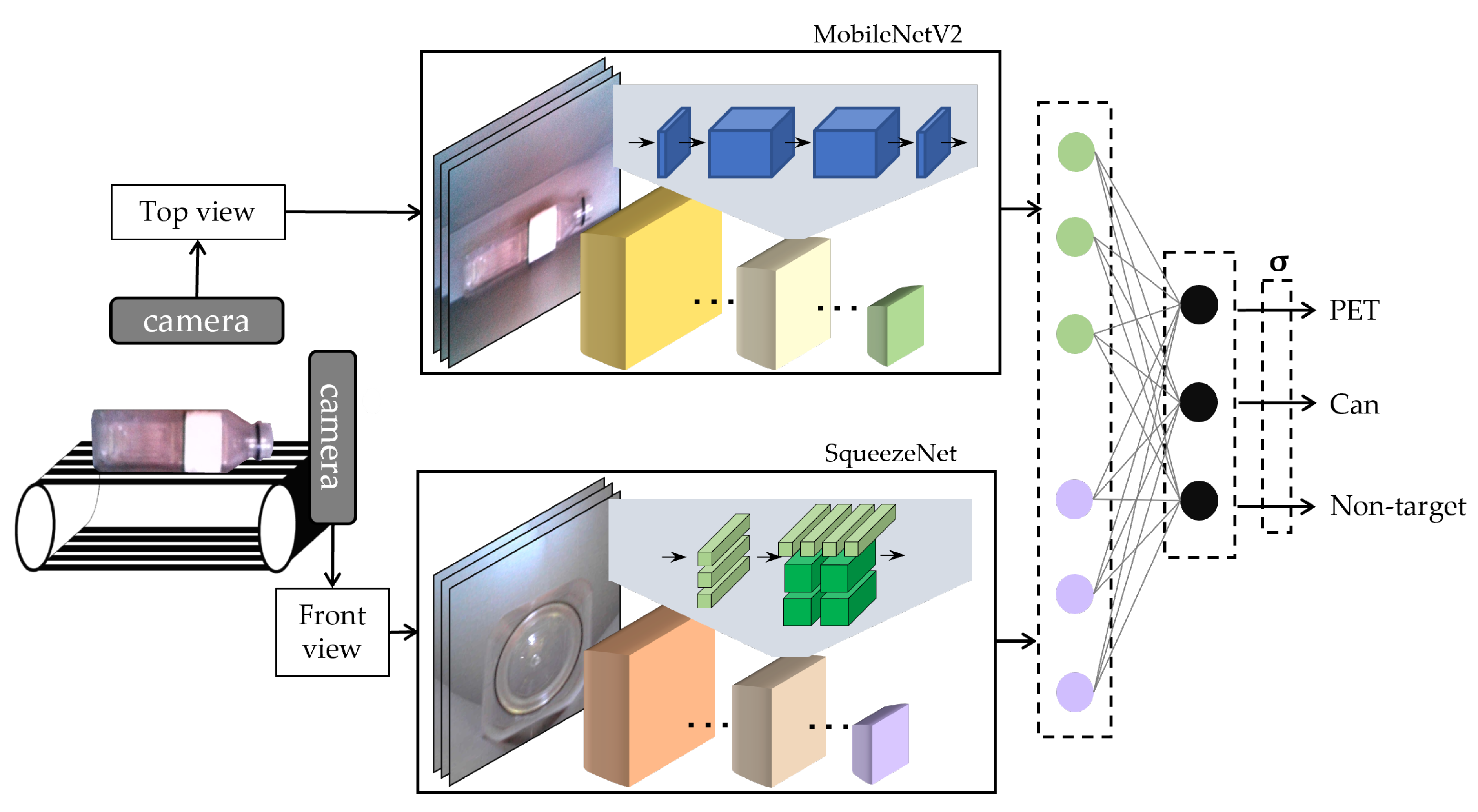
The final framework of the proposed CNN ensemble model can be represented as Figure 8. First, the top view image of the input object is classified through MobileNetV2, and the front view image is classified through SqueezeNet. Then, the prediction vectors generated by each classifier are concatenated and classified into PET, Can, and non-target classes through SLP. The following section describes the specific experimental results and discussions on our path to find the proposed model.
4. Experimental Results and Discussions
In this section, we present and discuss the experimental results. In every experiment, we used the deep learning library PyTorch [52] version 1.7.0 to implement and modify CNN models. These CNN models were pre-trained with the ImageNet and fine-tuned on NVIDIA GeForce RTX 2080 Super with 8 GB memory. As our performance metric, we chose classification accuracy, which represents the ratio between the number of correctly classified data and the entire dataset. Since we used a well-balanced dataset for multi-class classification, classification accuracy can be the most reasonable and straightforward performance metric [53].
4.1. Outline of Experiments
This study conducted three successive experiments to obtain the optimal CNN ensemble model. The experiments performed are summarized in Table 2. First, we classified data using only top view images in the PET and Can class, similar to the previous image-based RVM studies [12,13]. In the following experiment, we added a class representing a negative class, called the non-target, and classified the data using top view and front view images separately. From the experimental results, the candidates for the final ensemble model were narrowed down to the models with high classification accuracy and small model size. Next, we ensembled the CNNs selected from the previous experiment and chose the best-fit model by comparing the performance of the ensembles. Finally, we also evaluated the inference time of our best-fit CNN ensemble model in the NVIDIA Jetson Nano and TX1 Developer Kit.
As suggested in Section 3.3, to increase the prediction reliability, this study applied the decision threshold as secondary validation after picking the class with the maximum probability. The decision threshold is set to 0.5 by default, but the threshold value can vary on the application characteristics. For example, when we classify the objects into two classes, PET and Can, the maximum probability will always exceed 0.5. Thus we need a different threshold value to distinguish the non-target objects. In such a case, we used a heuristic threshold of 0.8 instead of the default threshold value. For the other experiments classifying the objects into PET, Can, and non-target classes, we applied the default threshold of 0.5.
4.2. Single Image-Based Classification
As a baseline experiment, we classified the object with only the top view image. This experiment was conducted in two steps. First, we trained the model without the non-target dataset and classified the object into two classes, PET and Can classes. Since the models used in the investigation do not produce the non-target class, we applied the decision threshold of 0.8 to distinguish the non-target objects in the secondary validation. Table 3 shows the results of this experiment. SqueezeNet and MobileNetV2 showed the highest and balanced accuracy among the candidate models, but their classification performance for non-target objects was unsatisfactory. Furthermore, when we further divide non-target objects into fraud and IAO, the accuracy on fraud objects is significantly lower than IAO. This result indicates that CNNs trained with our dataset also show erroneous classification results on non-target objects including fraud objects, as in the previous RVM study [14].
In the following experiment, we added the non-target class to improve the poor classification performance of non-target objects. Table 4 shows the results of the experiment. It is observed that the EfficientNet family and DenseNet have a lower classification accuracy of the Can class than the PET class, while SqueezeNet and MobileNetV2 show equally high accuracy for both classes. On the other hand, in the classification accuracy of the non-target class, all models showed better results than the first experiment. However, it is still not enough for a real-world RVM system.
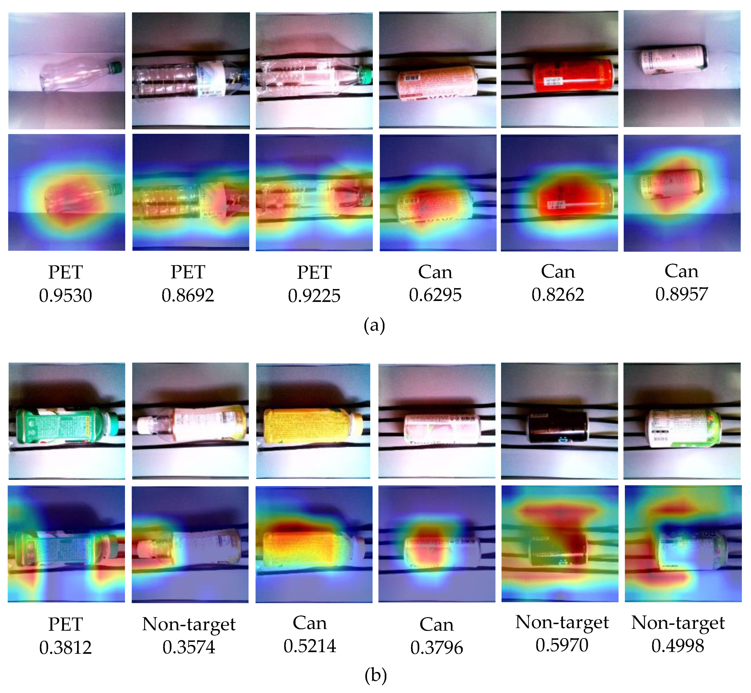
Comparing the results of SqueezeNet and MobileNetV2 in Table 3 and Table 4, we observe that adding a negative class improves the robustness against intentional frauds and unexpected inputs. However, it also degrades the accuracy of target object classification. Therefore, we further investigated using model visualization of which parts of the images the training models focus on to make the classification decision. As the model visualization method, we used the Gradient-weighted Class Activation Mapping (Grad-CAM) [54].
Figure 9a,b illustrate the Grad-CAM visualization results of correctly classified objects and incorrectly classified objects with the MobileNetV2 model, respectively. It shows that the trained MobileNetV2 concentrates on the neck and bottom part of the PET bottle rather than the label. So, it is challenging to classify a bottle with a short neck or a large label covering a whole part of the container. Contrarily, as for the aluminum cans, the model mainly focuses on the label but sometimes focuses on the shadows. Therefore, it becomes difficult for models to correctly identify an object of which the label has never been trained, and the illumination condition may also affect the result. From these observations, we need to find and use the common characteristics of PET bottles and aluminum cans other than the appearance or label and the shape of the neck or bottom part of the objects to achieve better interference results.
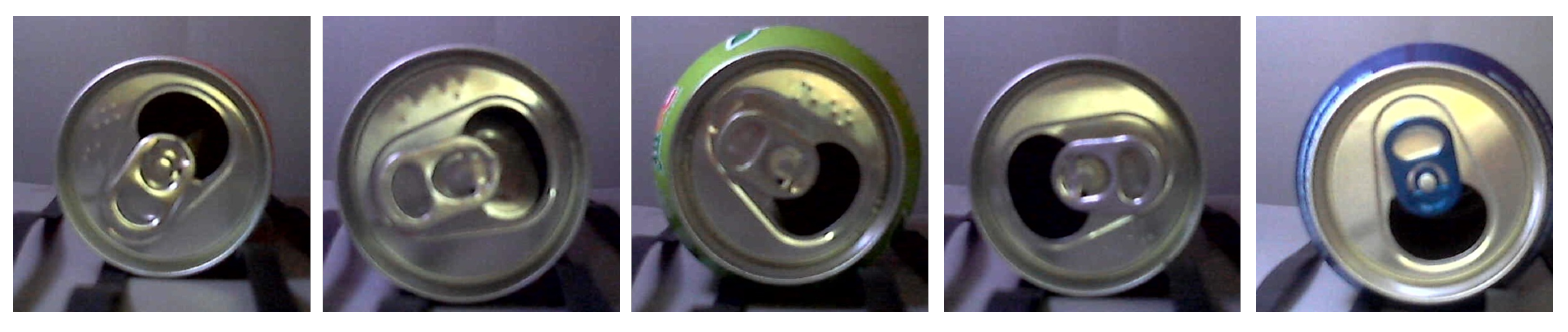
As shown in Figure 10, we can find that a common characteristic of most PET bottles and aluminum cans is the shape of the lid, which corresponds to the front view in our approach. Using this common feature, we tested the classification accuracy with only the front view images and show the results in Table 5. Since ResNet-18 has the largest model size among the candidate CNNs but is not showing acceptable classification performance, we excluded the ResNet-18 from subsequent experiments. The experimental results in Table 5 show that, as expected, training with the front view images is more accurate than the top view image training. The general accuracy of 100% on target objects is not surprising. Previous work by Park et al. [14] also presented the 99% classification accuracy of pet bottles, cans, and glasses, but they did not consider the fraud objects.
According to the classification accuracy of target objects, SqueezeNet and MobileNetV2 can be regarded as the best-fit models for the RVM application, as in the previous experiments. However, their accuracy for the fraud object is still low. Furthermore, creating an intentional fraud object of the front view is more straightforward than the top view.
4.3. Dual Image-Based Classification with CNN Ensemble Models
All previous experiments were conducted using only one cross-section of an object. Since the single view provides limited information about the object, the models trained in previous experiments produce erroneous predictions when classifying intentional fraud. To overcome this limitation and provide more details to the model, we used both the top view and the front view of input objects for training. We also constructed CNN ensemble models combining top view and front view classification results with a stacking ensemble scheme.
The CNN models for the final ensemble were chosen based on their classification accuracy and size. From the previous experimental results, SqueezeNet and MobileNetV2 showed consistently good classification accuracy over other models. They also have a noticeable advantage in lightweight embedded platforms because the models have fewer parameters than other models. For this reason, we constructed CNN ensemble models using SqueezeNet and MobileNetV2.
Table 6 shows the performance of four different CNN ensemble combinations from SqueezeNet and MobileNetV2. The results show that the best-fit ensemble model uses MobileNetV2 as the top view classifier and SqueezeNet as the front view classifier. The best-fit CNN ensemble model shows classification accuracy better than 95% for all the classes. Although the accuracy for the PET and the Can classes are slightly lower than the single CNN results in Table 5, we can consider this little performance degradation as a reasonable trade-off for the remarkable improvement in the accuracy for the fraud objects.
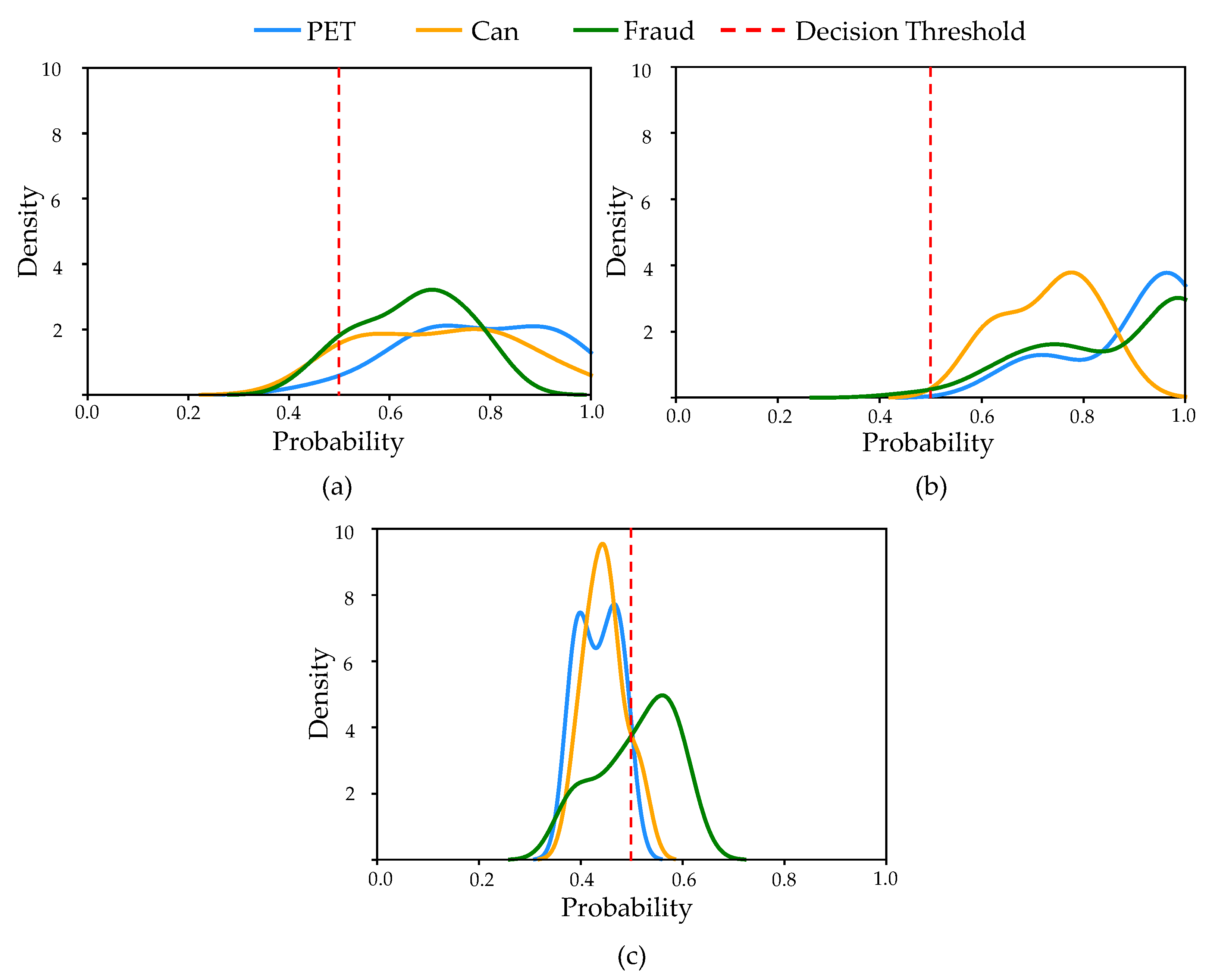
To analyze what makes our proposed CNN ensemble model produce more accurate classifications of fraud objects than a single CNN, we applied kernel density estimation to the prediction results of the fraud objects. Figure 11 illustrates the kernel density estimation of the fraud object predictions in our experiments. Figure 11a,b show the results of MobileNetV2 trained with only the top view or the front view image, respectively, and Figure 11c shows the result of the final CNN ensemble model. Figure 11a,b indicate that when MobileNetV2 incorrectly classifies a fraud object as PET or Can class after picking argmax, in most cases, prediction probabilities exceed the decision threshold of 0.5. This result leads to poor accuracy by finally misclassifying it as a legal target class.
Figure 11c shows that our proposed CNN ensemble model also incorrectly identifies fraud objects as legal target objects after argmax. However, even in an erroneous classification, the prediction probability is mostly lower than the decision threshold and is finally classified as a Non-target class. For this reason, the proposed CNN ensemble model can improve the detection rate of fraud objects. To summarize, the proposed CNN ensemble model shows better accuracy than single CNN models by lowering the confidence on fraud objects that are misclassified into target objects.
4.4. Performance on Embedded AI Platform
In the last stage of our experiment, we measured the inference time of the proposed CNN ensemble model on different edge AI devices to investigate the execution performance. NVIDIA Jetson Nano and TX1 platforms are employed for this experiment, and the platform specifications are summarized in Table 7. Both platforms equally used PyTorch version 1.7.0, CUDA version 10.2.89, and CuDNN version 8.0.0.180. We measured the inference time using CUDA Event class because CUDA functions are called asynchronously in PyTorch, and also we performed a sufficient GPU warm-up before measurement for precise measurement.
Table 8 shows a 99% confidence interval of inference time with 1182 measurements. We observed that the confidence intervals of Jetson Nano and TX1 are 67.25 ± 1.46 ms and 55.24 ± 1.2 ms, respectively. We then compared the results with a previous work by Liukkonen [10]. In [10], the sufficient throughput for the RVM system was suggested as 40.8 objects per minute, that is, the average processing time of 1470.56 ms per object. On the other hand, the performance of the state-of-the-art commercial RVMs [39,40] also amount to about 45 to 60 objects per minute. Our results in Table 8 indicate that with 99% confidence, the average inference time of our model will be below 70 ms, which is about 4.7∼7% of the total processing time in other RVMs. From the results, we consider that the inference time based on our proposed approach is fast enough to guarantee the real-time processing of object classification in RVMs.
5. Conclusions
Current RVMs and previous studies on waste classification have suffered from limited collection resource scope, high system configuration cost, and the erroneous prediction of intentional frauds. To tackle these problems, we proposed a CNN ensemble model that combines two CNN models trained for different views of objects using a stacking ensemble scheme. To this end, we first investigated the classification performance of popular CNN models based on the image dataset acquired from our prototype RVM. From the results, we notice that the single image-based classification approach is fragile to intentional fraud objects. Therefore, we attempted to use both the top view and the front view of objects and construct the ensemble models with the classifiers having good accuracy for single image-based training tests and small model sizes. As a result, we finally set up the best-fit ensemble model that uses MobileNetV2 as the top view classifier and SqueezeNet as the front view classifier.
The experimental results for the best-fit ensemble model derived in this study showed that our approach could produce classification accuracy higher than 95% for all target classes. In particular, our model significantly outperformed single image-based CNNs in classifying fraud objects. This improvement is due to two reasons. First, the dual image-based system provides more object information than the single image-based system and thus leads to better accuracy on target objects. Second, the confidence measure of intentional fraud objects is lower than the single image-based system, leading to better accuracy after passing the decision threshold layer. Furthermore, the proposed model presented an inference time of less than 70 ms on the NVIDIA Jetson platforms. This result also demonstrates that our model can achieve an execution performance comparable to a lightweight commercial RVM solution.
The future work includes using more than two different views, such as the top, front, and backward views. The use of multiple views can classify the object regardless of the input direction.
Author Contributions
Conceptualization, T.Y.; methodology, T.Y., S.L. and T.K.; experiment and analysis, T.Y.; supervision, T.K.; funding acquisition, T.K.; writing, T.Y., S.L. and T.K. All authors have read and agreed to the published version of the manuscript.
Funding
This work was financially supported by Korea Ministry of Land, Infrastructure and Transport(MOLIT) as “Innovative Talent Education Program for Smart City”.
Data Availability Statement
The dataset used in this paper is accessible on Github repository: https://github.com/taeyoungYoo/rvm-dataset (accessed on 15 November 2021).
Conflicts of Interest
The authors declare no conflict of interest.
Abbreviations
The following abbreviations are used in this manuscript:
| RVM | Reverse vending machine |
| PET | Polyethylene terephthalate |
| IoT | Internet of Things |
| CNN | Convolutional neural network |
| AI | Artificial intelligence |
| GPU | Graphics processing unit |
| Bagging | Bootstrap aggregating |
| IAO | Inappropriate object |
| ResNet | Residual neural network |
| DenseNet | Dense Convolutional Network |
| SLP | Single layer perceptron |
| Grad-CAM | Gradient-weighted Class Activation Mapping |
References
- Calcott, P.; Walls, M. Waste, recycling, and “Design for Environment”: Roles for markets and policy instruments. Resour. Energy Econ. 2005, 27, 287–305. [Google Scholar] [CrossRef] [Green Version]
- Reverse Vending 101: A Beginner’s Guide. Available online: https://newsroom.tomra.com/reverse-vending-101-a-beginners-guide/ (accessed on 15 November 2021).
- Amantayeva, A.; Alkuatova, A.; Kanafin, I.; Tokbolat, S.; Shehab, E. A systems engineering study of integration reverse vending machines into the waste management system of Kazakhstan. J. Mater. Cycles Waste Manag. 2021, 23, 872–884. [Google Scholar] [CrossRef]
- Pramita, S.; Mhatre, P.; Gowda, A.; Deeksha, R.; Srikanth, U. A Study on Challenges for Adoption of Reverse Vending Machine: A Case of North Bengaluru, India. In Proceedings of the World Conference on Waste Management, Colombo, Sri Lanka, 8 March 2019; Volume 1, pp. 15–29. [Google Scholar]
- Kabugu, S. Deposit-Refund System: Feasibility Study on How to Introduce a Deposit-Refund System in Nairobi, Kenya. 2015. Available online: https://www.theseus.fi/handle/10024/102585 (accessed on 15 November 2021).
- Esmaeilian, B.; Wang, B.; Lewis, K.; Duarte, F.; Ratti, C.; Behdad, S. The future of waste management in smart and sustainable cities: A review and concept paper. Waste Manag. 2018, 81, 177–195. [Google Scholar] [CrossRef] [PubMed]
- Aazam, M.; St-Hilaire, M.; Lung, C.H.; Lambadaris, I. Cloud-based smart waste management for smart cities. In Proceedings of the 2016 IEEE 21st International Workshop on Computer Aided Modelling and Design of Communication Links and Networks (CAMAD), Toronto, ON, Canada, 23–25 October 2016; pp. 188–193. [Google Scholar]
- Anagnostopoulos, T.; Zaslavsky, A.; Kolomvatsos, K.; Medvedev, A.; Amirian, P.; Morley, J.; Hadjieftymiades, S. Challenges and opportunities of waste management in IoT-enabled smart cities: A survey. IEEE Trans. Sustain. Comput. 2017, 2, 275–289. [Google Scholar] [CrossRef]
- Popa, C.L.; Carutasu, G.; Cotet, C.E.; Carutasu, N.L.; Dobrescu, T. Smart city platform development for an automated waste collection system. Sustainability 2017, 9, 2064. [Google Scholar] [CrossRef] [Green Version]
- Liukkonen, J. Machine Vision System for a Reverse Vending Machine. Master’s Thesis, School of Electrical Engineering, Aalto University, Espoo, Finland, 2015. [Google Scholar]
- Kavli, T.Ø.; Njåstad, J.; Saether, G. Method and Apparatus for Detecting Fraud Attempts in Reverse Vending Machines. U.S. Patent 9,189,911, 17 November 2015. [Google Scholar]
- Kokoulin, A.N.; Tur, A.I.; Yuzhakov, A.A. Convolutional neural networks application in plastic waste recognition and sorting. In Proceedings of the 2018 IEEE Conference of Russian Young Researchers in Electrical and Electronic Engineering (EIConRus), Moscow and St. Petersburg, Russia, 29 January–1 February 2018; pp. 1094–1098. [Google Scholar]
- Kokoulin, A.N.; Kiryanov, D.A. The Optical Subsystem for the Empty Containers Recognition and Sorting in a Reverse Vending Machine. In Proceedings of the 2019 4th International Conference on Smart and Sustainable Technologies (SpliTech), Split, Croatia, 18–21 June 2019; pp. 1–6. [Google Scholar] [CrossRef]
- Park, J.; Kim, M.H.; Choi, S.; Kweon, I.S.; Choi, D.G. Fraud detection with multi-modal attention and correspondence learning. In Proceedings of the 2019 International Conference on Electronics, Information, and Communication (ICEIC), Auckland, New Zealand, 22–25 January 2019; pp. 1–7. [Google Scholar]
- Sinaga, E.F.; Irawan, R. Developing barcode scan system of a small-scaled reverse vending machine to sorting waste of beverage containers. Telkomnika 2020, 18, 2087–2094. [Google Scholar] [CrossRef]
- Rahim, N.H.A.; Khatib, A.N.H.M. Development of PET bottle shredder reverse vending machine. Int. J. Adv. Technol. Eng. Explor. 2021, 8, 24. [Google Scholar] [CrossRef]
- Alzubaidi, L.; Zhang, J.; Humaidi, A.J.; Al-Dujaili, A.; Duan, Y.; Al-Shamma, O.; Santamaría, J.; Fadhel, M.A.; Al-Amidie, M.; Farhan, L. Review of deep learning: Concepts, CNN architectures, challenges, applications, future directions. J. Big Data 2021, 8, 1–74. [Google Scholar]
- LeCun, Y.; Bengio, Y.; Hinton, G. Deep learning. Nature 2015, 521, 436–444. [Google Scholar] [CrossRef] [PubMed]
- Albawi, S.; Mohammed, T.A.; Al-Zawi, S. Understanding of a convolutional neural network. In Proceedings of the 2017 International Conference on Engineering and Technology (ICET), Antalya, Turkey, 21–23 August 2017; pp. 1–6. [Google Scholar]
- Hansen, L.K.; Salamon, P. Neural network ensembles. IEEE Trans. Pattern Anal. Mach. Intell. 1990, 12, 993–1001. [Google Scholar] [CrossRef] [Green Version]
- Breiman, L. Bagging predictors. Mach. Learn. 1996, 24, 123–140. [Google Scholar] [CrossRef] [Green Version]
- Freund, Y.; Schapire, R.E. Experiments with a new boosting algorithm. In Proceedings of the ICML, Murray Hill, NJ, USA, 22 January 1996; Volume 96, pp. 148–156. [Google Scholar]
- Wolpert, D.H. Stacked generalization. Neural Netw. 1992, 5, 241–259. [Google Scholar] [CrossRef]
- Guo, J.; Gould, S. Deep CNN ensemble with data augmentation for object detection. arXiv 2015, arXiv:1506.07224. [Google Scholar]
- Zhou, Z.H.; Wu, J.; Tang, W. Ensembling neural networks: Many could be better than all. Artif. Intell. 2002, 137, 239–263. [Google Scholar] [CrossRef] [Green Version]
- Chen, Y.; Wang, Y.; Gu, Y.; He, X.; Ghamisi, P.; Jia, X. Deep learning ensemble for hyperspectral image classification. IEEE J. Sel. Top. Appl. Earth Obs. Remote Sens. 2019, 12, 1882–1897. [Google Scholar] [CrossRef]
- Antipov, G.; Berrani, S.A.; Dugelay, J.L. Minimalistic CNN-based ensemble model for gender prediction from face images. Pattern Recognit. Lett. 2016, 70, 59–65. [Google Scholar] [CrossRef]
- Manzo, M.; Pellino, S. Fighting together against the pandemic: Learning multiple models on tomography images for COVID-19 diagnosis. AI 2021, 2, 261–273. [Google Scholar] [CrossRef]
- Zheng, H.; Gu, Y. EnCNN-UPMWS: Waste Classification by a CNN Ensemble Using the UPM Weighting Strategy. Electronics 2021, 10, 427. [Google Scholar] [CrossRef]
- Li, H.; Ota, K.; Dong, M. Learning IoT in edge: Deep learning for the Internet of Things with edge computing. IEEE Netw. 2018, 32, 96–101. [Google Scholar] [CrossRef] [Green Version]
- Zhang, X.; Wang, Y.; Shi, W. pCAMP: Performance Comparison of Machine Learning Packages on the Edges. In USENIX Workshop on Hot Topics in Edge Computing (HotEdge 18); USENIX Association: Boston, MA, USA, 2018. [Google Scholar]
- Merenda, M.; Porcaro, C.; Iero, D. Edge machine learning for ai-enabled iot devices: A review. Sensors 2020, 20, 2533. [Google Scholar] [CrossRef]
- Taspinar, Y.S.; Selek, M. Object Recognition with Hybrid Deep Learning Methods and Testing on Embedded Systems. Int. J. Intell. Syst. Appl. Eng. 2020, 8, 71–77. [Google Scholar] [CrossRef]
- Antonini, M.; Vu, T.H.; Min, C.; Montanari, A.; Mathur, A.; Kawsar, F. Resource characterisation of personal-scale sensing models on edge accelerators. In Proceedings of the First International Workshop on Challenges in Artificial Intelligence and Machine Learning for Internet of Things, New York, NY, USA, 10 November 2019; pp. 49–55. [Google Scholar]
- Mittal, S. A Survey on optimized implementation of deep learning models on the NVIDIA Jetson platform. J. Syst. Archit. 2019, 97, 428–442. [Google Scholar] [CrossRef]
- Ullah, S.; Kim, D.H. Benchmarking Jetson platform for 3D point-cloud and hyper-spectral image classification. In Proceedings of the 2020 IEEE International Conference on Big Data and Smart Computing (BigComp), Busan, Korea, 19–22 February 2020; pp. 477–482. [Google Scholar]
- Koubaa, A.; Ammar, A.; Kanhouch, A.; Alhabashi, Y. Cloud versus Edge Deployment Strategies of Real-Time Face Recognition Inference. IEEE Trans. Netw. Sci. Eng. 2021. [Google Scholar] [CrossRef]
- Dataset for Waste Classification. Available online: https://github.com/taeyoungYoo/rvm-dataset (accessed on 15 November 2021).
- Reverse Vending Solution for Reverage Container Recycling. Available online: https://www.tomra.com/en/collection/reverse-vending/reverse-vending-systems (accessed on 15 November 2021).
- Reverse Vending Solutions: The First in-Store Customer Touchpoint—Designed to Protect the Environment. Available online: https://www.dieboldnixdorf.com/en-us/retail/portfolio/systems/reverse-vending-solutions (accessed on 15 November 2021).
- He, K.; Zhang, X.; Ren, S.; Sun, J. Deep residual learning for image recognition. In Proceedings of the IEEE Conference on Computer Vision and Pattern Recognition, Las Vegas, NV, USA, 27–30 June 2016; pp. 770–778. [Google Scholar]
- Huang, G.; Liu, Z.; van der Maaten, L.; Weinberger, K.Q. Densely Connected Convolutional Networks. In Proceedings of the IEEE Conference on Computer Vision and Pattern Recognition (CVPR), Honolulu, HI, USA, 21–26 July 2017. [Google Scholar]
- Iandola, F.N.; Han, S.; Moskewicz, M.W.; Ashraf, K.; Dally, W.J.; Keutzer, K. SqueezeNet: AlexNet-level accuracy with 50× fewer parameters and< 0.5 MB model size. arXiv 2016, arXiv:1602.07360. [Google Scholar]
- Sandler, M.; Howard, A.; Zhu, M.; Zhmoginov, A.; Chen, L.C. Mobilenetv2: Inverted residuals and linear bottlenecks. In Proceedings of the IEEE Conference on Computer Vision and Pattern Recognition, Salt Lake City, UT, USA, 18–23 June 2018; pp. 4510–4520. [Google Scholar]
- Howard, A.G.; Zhu, M.; Chen, B.; Kalenichenko, D.; Wang, W.; Weyand, T.; Andreetto, M.; Adam, H. Mobilenets: Efficient convolutional neural networks for mobile vision applications. arXiv 2017, arXiv:1704.04861. [Google Scholar]
- Tan, M.; Le, Q. EfficientNet: Rethinking Model Scaling for Convolutional Neural Networks. In Proceedings of the 36th International Conference on Machine Learning, Long Beach, CA, USA, 9–15 June 2019; Volume 97, pp. 6105–6114. [Google Scholar]
- Perez, F.; Avila, S.; Valle, E. Solo or ensemble? choosing a cnn architecture for melanoma classification. In Proceedings of the IEEE/CVF Conference on Computer Vision and Pattern Recognition Workshops, Long Beach, CA, USA, 16–17 June 2019. [Google Scholar]
- Dietterich, T.G. An experimental comparison of three methods for constructing ensembles of decision trees: Bagging, boosting, and randomization. Mach. Learn. 2000, 40, 139–157. [Google Scholar] [CrossRef]
- Divina, F.; Gilson, A.; Goméz-Vela, F.; García Torres, M.; Torres, J.F. Stacking ensemble learning for short-term electricity consumption forecasting. Energies 2018, 11, 949. [Google Scholar] [CrossRef] [Green Version]
- Ting, K.M.; Witten, I.H. Issues in stacked generalization. J. Artif. Intell. Res. 1999, 10, 271–289. [Google Scholar] [CrossRef] [Green Version]
- Džeroski, S.; Ženko, B. Is combining classifiers with stacking better than selecting the best one? Mach. Learn. 2004, 54, 255–273. [Google Scholar] [CrossRef] [Green Version]
- Paszke, A.; Gross, S.; Massa, F.; Lerer, A.; Bradbury, J.; Chanan, G.; Killeen, T.; Lin, Z.; Gimelshein, N.; Antiga, L. Pytorch: An imperative style, high-performance deep learning library. Adv. Neural Inf. Process. Syst. 2019, 32, 8026–8037. [Google Scholar]
- Chicco, D.; Jurman, G. The advantages of the Matthews correlation coefficient (MCC) over F1 score and accuracy in binary classification evaluation. BMC Genom. 2020, 21, 1–13. [Google Scholar] [CrossRef] [PubMed] [Green Version]
- Selvaraju, R.R.; Cogswell, M.; Das, A.; Vedantam, R.; Parikh, D.; Batra, D. Grad-cam: Visual explanations from deep networks via gradient-based localization. In Proceedings of the IEEE International Conference on Computer Vision, Venice, Italy, 22–29 October 2017; pp. 618–626. [Google Scholar]
Figure 1.
Workflow of choosing optimized classifiers and framework of the proposed CNN ensemble model.
Figure 1.
Workflow of choosing optimized classifiers and framework of the proposed CNN ensemble model.

Figure 2.
Hardware setup for constructing dataset: (a) Prototype RVM; (b) Settings for capturing dual image.
Figure 2.
Hardware setup for constructing dataset: (a) Prototype RVM; (b) Settings for capturing dual image.

Figure 3.
Dataset and its composition.

Figure 4.
Actual images from the dataset: (a) Top view of PET and Can classes; (b) Top view of Non-target class with printed images of PET and can, PET label-only object, and IAO such as paper cup; (c) Front view of PET and Can classes; (d) Front view of Non-target class with printed images of PET and can, and IAO such as whiteboard eraser.

Figure 5.
Building blocks of ResNet and DenseNet: (a) Bottleneck building block for ResNet 50/101/152 where the 1 × 1 layers reduce and increase dimensions, and 3 × 3 layer extracts features; (b) Simple dense block of DenseNet. The multiple dense blocks are connected with the transition layers and compose the DenseNet.

Figure 6.
Building blocks of SqueezeNet and MobileNetV2: (a) Fire module of SqueezeNet with three 1 × 1 convolutional filters in the squeeze layer, four 1 × 1 convolutional filters in the expand layer, and four 3 × 3 convolutional filters in the expand layer; (b) Bottleneck depthwise separable convolution with residuals, which is a basic building block of MobileNetV2. This figure represents the block where .

Figure 7.
Simple scheme of stacking ensemble learning procedure.

Figure 8.
Framework of the proposed CNN ensemble model.

Figure 9.
Grad-CAM visualization results using MobileNetV2 for target objects: (a) Properly classified objects; (b) Misclassified objects. The predicted class and its probability are shown below each Grad-CAM figure.
Figure 9.
Grad-CAM visualization results using MobileNetV2 for target objects: (a) Properly classified objects; (b) Misclassified objects. The predicted class and its probability are shown below each Grad-CAM figure.

Figure 10.
Front view of five different aluminum cans.

Figure 11.
Kernel density estimation for prediction result of fraud objects: (a) MobileNetV2 trained only with top view images; (b) MobileNetV2 trained only with front view images; (c) The proposed CNN ensemble model.
Figure 11.
Kernel density estimation for prediction result of fraud objects: (a) MobileNetV2 trained only with top view images; (b) MobileNetV2 trained only with front view images; (c) The proposed CNN ensemble model.


Table 1.
Classes and objects used in this study. The composition of objects is same on both the top view and the front view.
Table 1.
Classes and objects used in this study. The composition of objects is same on both the top view and the front view.
| Class | Objects |
|---|---|
| PET | PET bottles with or without labels, and with or without caps |
| Can | Aluminum cans with or without lids |
| Non-target | Printed PET bottles, cans, and PET label-only objects (fraud objects). Human hands, roll papers, paper box, etc (IAOs). |
Table 2.
Details of our experiments to find optimized classifiers.
| Step | Network | Input Image | Decision Threshold | Class |
|---|---|---|---|---|
| (1) | Single CNN | Top view only | 0.8 | PET, Can |
| (2) | Single CNN | Top view only | 0.5 | PET, Can, Non-target |
| (3) | Single CNN | Front view only | 0.5 | PET, Can, Non-target |
| (4) | CNN Ensemble Model | Top view and Front view at once | 0.5 | PET, Can, Non-target |
Table 3.
Performance of CNNs trained with top view data, classifying objects into PET and Can classes. Heuristic threshold has been applied to distinguish non-target objects.
Table 3.
Performance of CNNs trained with top view data, classifying objects into PET and Can classes. Heuristic threshold has been applied to distinguish non-target objects.
| Model | #Params | PET | Can | Non-Target | |
|---|---|---|---|---|---|
| Fraud | IAO | ||||
| ResNet-18 | 11.2M | 86.36% | 87.88% | 22.86% | 60.00% |
| DenseNet-121 | 7.0M | 97.73% | 77.27% | 10.00% | 71.67% |
| SqueezeNet | 0.7 M | 93.94% | 92.42% | 14.29% | 18.33% |
| MobileNetV2 | 2.2 M | 93.94% | 90.91% | 24.29% | 43.33% |
| EfficientNet-B0 | 4.0 M | 89.39% | 45.45% | 34.29% | 78.33% |
| EfficientNet-B1 | 6.5 M | 65.15% | 33.33% | 45.71% | 75.00% |
| EfficientNet-B2 | 7.7M | 76.52% | 42.42% | 40.00% | 73.33% |
Table 4.
Performance of CNNs trained with top view data, classifying objects into PET, Can, and non-target classes.
Table 4.
Performance of CNNs trained with top view data, classifying objects into PET, Can, and non-target classes.
| Model | #Params | PET | Can | Non-Target | |
|---|---|---|---|---|---|
| Fraud | IAO | ||||
| ResNet-18 | 11.2M | 89.39% | 88.64% | 44.29% | 88.33% |
| DenseNet-121 | 7.0M | 100.00% | 79.55% | 47.14% | 96.67% |
| SqueezeNet | 0.7 M | 90.15% | 90.91% | 52.86% | 63.33% |
| MobileNetV2 | 2.2 M | 93.18% | 88.64% | 41.43% | 85.00% |
| EfficientNet-B0 | 4.0 M | 95.45% | 66.67% | 37.14% | 75.00% |
| EfficientNet-B1 | 6.5 M | 79.55% | 67.42% | 47.14% | 90.00% |
| EfficientNet-B2 | 7.7M | 85.61% | 71.21% | 48.57% | 90.00% |
Table 5.
Performance of CNNs trained with front view data, classifying objects into PET, Can, and Non-target classes.
Table 5.
Performance of CNNs trained with front view data, classifying objects into PET, Can, and Non-target classes.
| Model | #Params | PET | Can | Non-Target | |
|---|---|---|---|---|---|
| Fraud | IAO | ||||
| DenseNet-121 | 7.0 M | 100.00% | 99.24% | 31.43% | 100.00% |
| SqueezeNet | 0.7 M | 100.00% | 100.00% | 34.29% | 100.00% |
| MobileNetV2 | 2.2 M | 93.18% | 100.00% | 61.43% | 100.00% |
| EfficientNet-B0 | 4.0 M | 83.33% | 100.00% | 70.00% | 100.00% |
| EfficientNet-B1 | 6.5 M | 68.94% | 100.00% | 68.57% | 93.33% |
| EfficientNet-B2 | 7.7 M | 93.18% | 100.00% | 47.14% | 100.00% |
Table 6.
Performance of CNN ensemble models trained with top view and front view data simultaneously, classifying objects into PET, Can, and non-target classes.
Table 6.
Performance of CNN ensemble models trained with top view and front view data simultaneously, classifying objects into PET, Can, and non-target classes.
| Top view | Front view | #Params | PET | Can | Non-Target | |
|---|---|---|---|---|---|---|
| Fraud | IAO | |||||
| MobileNetV2 | SqueezeNet | 2.96 M | 97.73% | 95.45% | 97.14% | 100.00% |
| MobileNetV2 | MobileNetV2 | 4.46 M | 87.88% | 95.45% | 95.71% | 100.00% |
| SqueezeNet | SqueezeNet | 1.47 M | 90.15% | 92.42% | 98.57% | 100.00% |
| SqueezeNet | MobileNetV2 | 2.96 M | 87.12% | 92.42% | 81.43% | 100.00% |
Table 7.
Specification of Jetson Nano and Jetson TX1.
| Platform | Jetson Nano | Jetson TX1 |
|---|---|---|
| GPU | 128-core NVIDIA Maxwell | 256-core NVIDIA Maxwell |
| CPU | Quad-Core ARM Cortex-A57 @1.42 GHz | Quad-Core ARM Cortex-A57 @1.73 GHz |
| Memory | 4GB 64-bit LPDDR4 | 4GB 64-bit LPDDR4 |
| AI Performance | 472 GFLOPs | 1.0 TFLOPs |
| Size | 100 mm × 80 mm × 29 mm | 170 mm × 170 mm × 15 mm |
| Price | USD 99 | USD 480 |
Table 8.
The proposed model’s inference time on Jetson Nano and Jetson TX1. The unit of inference time is ms.
Table 8.
The proposed model’s inference time on Jetson Nano and Jetson TX1. The unit of inference time is ms.
| Platform | Mean | Standard Deviation | 99% Confidence Interval | |
|---|---|---|---|---|
| Lower Bound | Upper Bound | |||
| Jetson Nano | 67.25 | 19.54 | 65.79 | 68.72 |
| Jetson TX1 | 55.24 | 16.01 | 54.04 | 56.44 |
Publisher’s Note: MDPI stays neutral with regard to jurisdictional claims in published maps and institutional affiliations. |
© 2021 by the authors. Licensee MDPI, Basel, Switzerland. This article is an open access article distributed under the terms and conditions of the Creative Commons Attribution (CC BY) license (https://creativecommons.org/licenses/by/4.0/).
Share and Cite
MDPI and ACS Style
Yoo, T.; Lee, S.; Kim, T. Dual Image-Based CNN Ensemble Model for Waste Classification in Reverse Vending Machine. Appl. Sci. 2021, 11, 11051. https://0-doi-org.brum.beds.ac.uk/10.3390/app112211051
AMA Style
Yoo T, Lee S, Kim T. Dual Image-Based CNN Ensemble Model for Waste Classification in Reverse Vending Machine. Applied Sciences. 2021; 11(22):11051. https://0-doi-org.brum.beds.ac.uk/10.3390/app112211051
Chicago/Turabian StyleYoo, Taeyoung, Seongjae Lee, and Taehyoun Kim. 2021. "Dual Image-Based CNN Ensemble Model for Waste Classification in Reverse Vending Machine" Applied Sciences 11, no. 22: 11051. https://0-doi-org.brum.beds.ac.uk/10.3390/app112211051
Note that from the first issue of 2016, this journal uses article numbers instead of page numbers. See further details here.