Resonance in the Cart-Pendulum System—An Asymptotic Approach

Abstract

The major objective of this research is to study the planar dynamical motion of 2DOF of an auto-parametric pendulum attached with a damped system. Using Lagrange’s equations in terms of generalized coordinates, the fundamental equations of motion (EOM) are derived. The method of multiple scales (MMS) is applied to obtain the approximate solutions of these equations up to the second order of approximation. Resonance cases are classified, in which the primary external and internal resonance are investigated simultaneously to establish both the solvability conditions and the modulation equations. In the context of the stability conditions of these solutions, the equilibrium points are obtained and graphically displayed to derive the probable steady-state solutions near the resonances. The temporal histories of the attained results, the amplitude, and the phases of the dynamical system are depicted in graphs to describe the motion of the system at any instance. The stability and instability zones of the system are explored, and it is discovered that the system’s performance is stable for a significant number of its variables.

1. Introduction

The motion of vibrating systems is regarded as one of the most significant motions in mechanics because of its numerous applications in life, such as in building structures, ships, rotor dynamics, sieves, pumps, compressors and transportation devices [1,2,3].

One of the most important systems is an auto-parametric one, which consists of at least two nonlinearly connected subsystems. The first subsystem can be excited by an external harmonic force when it is attached to a second one, which is known by an absorber. Therefore, one can determine the principal parametric resonance of the second subsystem (auto-parametric interaction) by reducing the response of the first subsystem, as seen in [4,5,6,7,8,9,10].

Fractional calculus has been used extensively during the last two decades in many branches of science and engineering [11,12,13,14]. In [11], the authors studied the dynamical motion of a particle in a circular cavity with aid of fractional calculus. The obtained fractional Hamilton’s EOM was explored using two approaches and was solved numerically. In [12,14], the authors studied the problems of a spring pendulum and two rigid pendulums having the same arm, connected with each other by a spring. The fractional Euler-Lagrange’s equation was derived and solved numerically for some fractional orders and initial conditions. The same concept of the fractional calculus is used in [13] to investigate the governing equation of motion for a capacitor microphone.

The behavior of a nonlinear damping 2DOF for a dynamical vibrating system connected with a spring is investigated in [7]. In [8], the authors studied a dynamical system of 4DOF consisting of an auto-parametric pendulum with a rigid body. The dynamic response of auto-parametric system under the influence of kinematic excitation was investigated numerically and experimentally in [9]. The authors studied whether the motion of the system was regular using plots. In [10], the authors studied the response of an auto-parametric system consisting of a pendulum absorber attached to a damping oscillatory system. The approximate solution near resonance was obtained using the method of harmonic balance [4]. The MMS was utilized in [15] to obtain the auto-parametric conditions of a damped Duffing system connected with a pendulum. By virtue of this technique, the solution of two coupled mass springs was obtained in [16]. The author discussed new excitation conditions in the presence of auto-parametric resonance. The auto-parametric resonance of a vibrating system under a third-order nonlinear coupling term was investigated in [17]. The bifurcation and the stability of a similar system under external forces was investigated in [18,19].

Moreover, MMS was utilized in [20] to obtain an autonomous system up to the third-order of the motion of a suspended point of a spring on a circular path. The fourth-order Runge-Kutta algorithm of ode45 solver [21] was applied in [22] to obtain the numerical solutions of the problem of a vibrating rigid body using Matlab packages. The obtained results were more consistent than previous works. The response of a harmonically damped spring pendulum was investigated in [23]; its suspended point followed an elliptic rout with a constant angular velocity. The MMS was utilized to obtain the resonance cases and to establish equations of modulation that identified all feasible steady-state solutions. The generalization of this model was presented in [24,25], where a rigid body was connected to a spring in the presence of a linear force along the spring’s arm. In addition, there were two moments, one at the point where the body connects to the spring and the other at the point when the pendulum is suspended. The external resonances were studied, and the solvability conditions were established. The comparison between both the numerical solutions of the governing EOM and the approximate ones showed high consistency between them. The oscillations of a spring pendulum in a fluid under the influence of buoyancy and drag forces in the presence of a harmonically external force were presented recently in [26]. The authors utilized the conditions of Routh-Hurwitz to investigate the stabilities of the steady-state solutions. In addition, the nonlinear stability analysis technique was used to determine the impact of various physical parameters on the motion.

On the other hand, the vibrational motions must be controlled in engineering applications through the existence of active and passive absorbers to avoid disturbance and devastation of the structures or the studied systems. Many works have studied such motions, e.g., [23,24,25,26,27,28,29,30,31]. In [29,30], the authors investigated a system consisting of a simple pendulum and a longitudinally tuned absorber. This system was subjected to an active control, such as negative values of velocity and angular displacement or their squares or even cubic values. The desired approximate solutions using MMS were obtained. The system’s stability, as well as the effects of absorbers on its behavior, were investigated. The behavior of 2DOF nonlinear spring pendulum was investigated in [31] at different resonance conditions and in the presence of both active and passive control.

The remainder of this paper is as follows: In Section 2, the motion of a 2DOF dynamical model consisting of a mass $M$ coupled to a damped spring and attached to a rigid arm of mass $m$ and length $\mathrm{l}$ is explored. The inspected motion is examined in the presence of a harmonic force $F$ that acts on the other end of the arm. Employing Lagrange’s equations, the EOM are derived. In Section 3, the MMS is used to achieve the solutions of the EOM up to the second order of approximation. In Section 4, resonance cases of the system are classified. Moreover, both the amplitude and phase variables are checked to investigate the stability conditions of the steady-state solutions. In Section 5, a the results are presented through a representation of the variations of the attained solutions for different parameters, using plots to demonstrate the effect of applied forces and other settings on the motion of the model under consideration. In Section 6, the system’s stability and instability areas are examined, in which it is found that the system’s behavior is stable for a large number of variables. Finally, the manuscript ends with concluding remarks.

The significant impetus for this effort stems from its numerous scientific uses, including instrumentation, addressing vibrations in railway vehicles, and the use of pendulum dampers in a variety of applications.

2. Formulation of the Problem

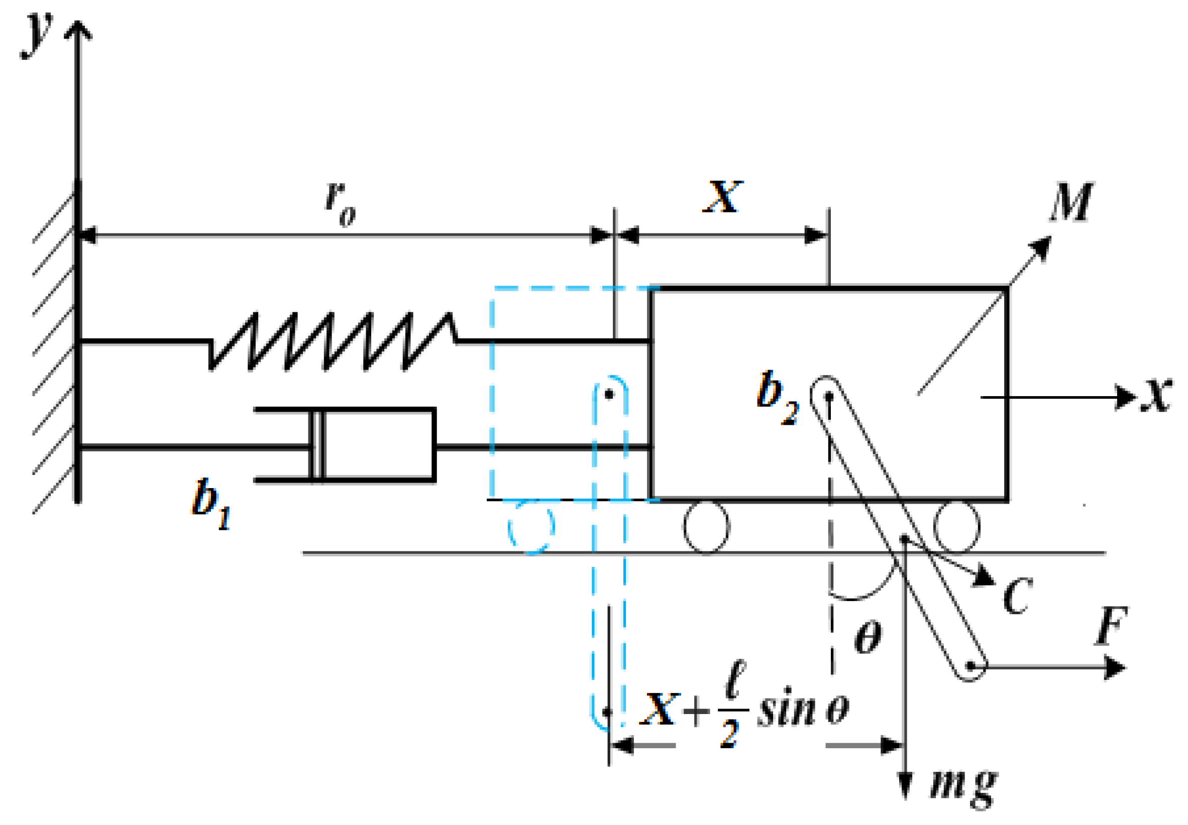
Let us consider a dynamical model consisting of mass $M$ connected with a spring of stiffness $k$ with linear stiffness $k X$. It is also attached to a linear damper with damping coefficient $b_1$ in translation. A uniform link of mass $m$ and length $\mathrm{l}$ is hinged to $M$ at the upper end, with linear viscous damping $b_2$ in rotation. The mechanical system is also influenced by a horizontal external harmonic force $F(t)$ at the lower end, as seen in Figure 1. Therefore, the motion can be characterized by the generalized coordinates $X(t)$ (translation of $M$) and $\theta (t)$ (rotation of the link).

Let $L=T-V$ denote the Lagrange’s function, in which $T$ and $V$ are the preceding model’s kinetic and potential energies that have the forms

$$\begin{array}{l}T=\frac{1}{2}(m v_C^2+M {\dot{X}}^2+I_C{\dot{\theta }}^2),\\ V=\frac{1}{2}[k X^2+mg\mathrm{l}(1-cos\theta )],\end{array}$$

(1)

where $g$ denotes the gravitational acceleration, $I_C=(m{\mathrm{l}}^2/12)$ represents the inertia moment and $v_C$ is the velocity at $C$ of the link. It is worthy to mention that the potential energy $V$ is the sum of potential energies due to the spring’s elongation and the gravitational force of the link.

In the represented model, $(X,\theta )$ and $(\dot{X},\dot{\theta })$ denote the generalized coordinates of our model and their corresponding generalized velocities. Consequently, Lagrange’s equations have the forms

$$\begin{array}{l}\frac{d}{dt}(\frac{\partial L}{\partial \dot{X}})-\frac{\partial L}{\partial X}=F(t)-b_1\dot{X},\\ \frac{d}{dt}(\frac{\partial L}{\partial \dot{\theta }})-\frac{\partial L}{\partial \theta }=F(t)\mathrm{l}\cos \theta -b_2\dot{\theta },\end{array}$$

(2)

where $F(t)=F^{*}\cos (\Omega t)$ with an excitation frequency $\Omega$ and amplitude $F^{*}$.

Substituting (1) into (2), one obtains the following governing equations

$$(M+m)\ddot{X}+\frac{1}{2}m\mathrm{l}(\ddot{\theta }\cos \theta -{\dot{\theta }}^2\sin \theta )+kX+b_1\dot{X}=F^{*}\cos \Omega t,$$

(3)

$$\frac{m}{3}{\mathrm{l}}^2\ddot{\theta }+\frac{m}{2}\mathrm{l}(\ddot{X}\cos \theta +g\sin \theta )+b_2\dot{\theta }=F^{*}\mathrm{l}\cos \Omega t\cos \theta ,$$

(4)

It is obvious that the previous two equations represent second-order differential equations for the generalized coordinates $X$ and $\theta$.

Let us consider the following parameters

$$\begin{array}{l}\tau ={\omega }_{1}t, \xi (\tau )=\frac{X(\tau )}{\mathrm{l}}, (M+m)=J, f=\frac{F^{*}}{J\mathrm{l}{\omega }_1^2}, \mu =\frac{m}{2J},\\ c_1=\frac{b_1}{J{\omega }_1}, c_2=\frac{b_2}{I{\omega }_1}, {\omega }_1^2=\frac{k}{J}, p=\frac{\Omega }{{\omega }_1}, I=\frac{m{\mathrm{l}}^2}{3},\\ \alpha =\frac{J{\mathrm{l}}^2}{I}, K=\frac{{\omega }_2}{{\omega }_1}, {\omega }_2^2=\frac{gm\mathrm{l}}{2I}.\end{array}$$

(5)

to convert (3) and (4) into the following forms

$$\ddot{\xi }(\tau )+c_1\dot{\xi }(\tau )+\xi (\tau )+\mu [\ddot{\theta }(\tau )\cos \theta (\tau )-{\dot{\theta }}^2(\tau )\sin \theta (\tau )]=f\cos (p\tau ),$$

(6)

$$\ddot{\theta }(\tau )+c_2\dot{\theta }(\tau )+\mu \alpha \ddot{\xi }(\tau )\cos \theta (\tau )+K^2\sin \theta (\tau )=f\alpha \cos (p\tau )\cos \theta (\tau ).$$

(7)

We limit our research to small deflections, so the trigonometric functions $\cos \theta$ and $\sin \theta$ can be approximated to $1$ and $\theta$, respectively, to yield

$$\ddot{\xi }(\tau )+c_1\dot{\xi }(\tau )+\xi (\tau )+\mu [\ddot{\theta }(\tau )-{\dot{\theta }}^2(\tau )\theta (\tau )]=f\cos (p\tau ),$$

(8)

$$\ddot{\theta }(\tau )+K^2\theta (\tau )+c_2\dot{\theta }(\tau )+\mu \alpha \ddot{\xi }(\tau )=f\alpha \cos (p\tau ).$$

(9)

Now, let us introduce a small parameter $(0<\epsilon \ll 1)$ according to

$$c_1=\epsilon {\widehat{c}}_1, c_2=\epsilon {\widehat{c}}_2, \mu =\epsilon \widehat{\mu }, f={\epsilon }^2\widehat{f}.$$

(10)

Substituting (10) into (8) and (9), we obtain the following forms of the EOM:

$$\ddot{\xi }(\tau )+\epsilon {\widehat{c}}_1\dot{\xi }(\tau )+\xi (\tau )+\epsilon \widehat{\mu } [\ddot{\theta }(\tau )-{\dot{\theta }}^2(\tau )\theta (\tau )]={\epsilon }^2\widehat{f}\cos (p\tau ),$$

(11)

$$\ddot{\theta }(\tau )+K^2\theta (\tau )+\epsilon {\widehat{c}}_2\dot{\theta }(\tau )+\epsilon \widehat{\mu }\alpha \ddot{\xi }(\tau )={\epsilon }^2\widehat{f}\alpha \cos (p\tau ).$$

(12)

The above Equations (11) and (12) represent second-order nonlinear differential equations in terms of $\xi$ and $\theta$.

3. The Announced Method

In this section, the MMS perturbation technique will be utilized to solve the governing EOM (11) and (12) up to the second order of approximation. Therefore, we need only three time scales, having the forms $T_0=\tau , T_1=\epsilon \tau ,$ and $T_2={\epsilon }^2\tau$. According to the procedure of MMS, we express $\xi$ and $\theta$ in powers of $\epsilon$ as

$$\begin{array}{l}\xi ={\xi }_0(T_0,T_1,T_2)+\epsilon {\xi }_1(T_0,T_1,T_2)+{\epsilon }^2{\xi }_2(T_0,T_1,T_2)+...,\\ \theta ={\theta }_0(T_0,T_1,T_2)+\epsilon {\theta }_1(T_0,T_1,T_2)+{\epsilon }^2{\theta }_2(T_0,T_1,T_2)+....\end{array}$$

(13)

Here, $T_0$ and $T_1,T_2$ are the fast and slow time scales, respectively. The time derivatives included in (11) and (12) are expressed according to the following operators:

$$\begin{array}{l}\frac{d}{d\tau }=D_0+\epsilon D_1+{\epsilon }^2{D}_2+...,\\ \frac{d^2}{d{\tau }^2}=D_0^2+2\epsilon D_0{D}_1+{\epsilon }^2(2D_0{D}_2+D_1^2)+...,\end{array}$$

(14)

where $D_n=\frac{\partial }{\partial T_n}; n=0,1,2$.

Substituting (13) into (11) and (12), using (14), and grouping the coefficients of equal powers of $\epsilon$ in both sides yields the next three sets, containing the following six partial differential equations (PDEs):

Order of${\epsilon }^0$

$$\begin{array}{l}{D}_0^2{\xi }_0+{\xi }_0=0,\\ D_0^2{\theta }_0+K^2{\theta }_0=0.\end{array}$$

(15)

Order of$\epsilon$

$$\begin{array}{l}{D}_0^2{\xi }_1+{\xi }_1=\widehat{\mu }{\theta }_0{(D_0{\theta }_0)}^2-2D_0{D}_1{\xi }_0-{\widehat{c}}_1{D}_0{\xi }_0-\widehat{\mu }{D}_0^2{\theta }_0,\\ D_0^2{\theta }_1+K^2{\theta }_1=-2D_0{D}_1{\theta }_0-{\widehat{c}}_2{D}_0{\theta }_0-\alpha \widehat{\mu }{D}_0^2{\xi }_0.\end{array}$$

(16)

Order of${\epsilon }^2$

$$\begin{array}{l}{D}_0^2{\xi }_2+{\xi }_2=-2D_0{D}_1{\xi }_1-(2D_0{D}_2+D_1^2){\xi }_0-{\widehat{c}}_1(D_0{\xi }_1+D_1{\xi }_0)\\ -\widehat{\mu }(D_0^2{\theta }_1+2D_0{D}_1{\theta }_0)+\widehat{\mu }[2{\theta }_0{D}_0{\theta }_0{D}_0{\theta }_1+2{\theta }_0{D}_0{\theta }_0{D}_1{\theta }_0\\ +{\theta }_1{(D_0{\theta }_0)}^2]+\widehat{f}\cos (p{T}_0),\\ D_0^2{\theta }_2+K^2{\theta }_2=-2D_0{D}_1{\theta }_1-(2D_0{D}_2+D_1^2){\theta }_0-{\widehat{c}}_2(D_0{\theta }_1+D_1{\theta }_0)\\ -\alpha \widehat{\mu }(D_0^2{\xi }_1+2D_0{D}_1{\xi }_0)+\alpha \widehat{f}\cos (p{T}_0).\end{array}$$

(17)

It is worthy to notice that the system in Equations (11) and (12) can be approximated by the above systems in Equations (15)–(17) of PDEs, which can be solved successively. Solutions of these equations starting from the zero approximation equations can be inserted into the next higher orders of approximation. Equations of system (15) are mutually independent homogenous equations. Consequently, their solutions are harmonic and can be expressed in their exponential forms as

$${\xi }_0=A(T_1,T_2)e^{i{T}_0}+\overline{A}(T_1,T_2)e^{-i{T}_0},$$

(18)

$${\theta }_0=B(T_1,T_2)e^{iK{T}_0}+\overline{B}(T_1,T_2)e^{-iK{T}_0},$$

(19)

where $A,B$ are determinable complex functions from the elimination of the secular terms and $\overline{A},\overline{B}$ are the corresponding complex conjugate.

It is obvious that the solutions of (16) and (17) depend on the solutions of (18) and (19) to some extent. Therefore, substituting (18) and (19) into the system of Equation (16), we remove the produced secular terms to gain the removable conditions in the forms

$$2D_{1}A+{\widehat{c}}_{1}A=0,$$

(20)

$$2D_{1}B+{\widehat{c}}_{2}B=0.$$

(21)

Therefore, the first-order approximations of the solutions have the forms

$${\xi }_1=\frac{\widehat{\mu }{B}^3{K}^2}{(9K^2-1)}{e}^{3iK{T}_0}-\frac{\widehat{\mu }{K}^{2}B(B\overline{B}+1)}{(K^2-1)}{e}^{iK{T}_0}+CC,$$

(22)

$${\theta }_1=\frac{\alpha \widehat{\mu }A}{(K^2-1)}{e}^{i{T}_0}+CC.$$

(23)

where $CC$ stands for the complex conjugate of the preceding terms. This symbol allows presentation of the long term and thus will be used frequently.

Substituting the solutions (18), (19), (22), and (23) into the system of Equation (17) and eliminating terms leads to secular ones, yielding

$$2i{D}_{2}A+D_1^{2}A+{\widehat{c}}_1{D}_{1}A-\frac{{\widehat{\mu }}^2\alpha A}{(K^2-1)}(1+2B\overline{B}{K}^2)=0,$$

(24)

$$2iK{D}_{2}B+D_1^{2}B+{\widehat{c}}_2{D}_{1}B+\frac{{\widehat{\mu }}^2{K}^4\alpha B}{(K^2-1)}(1+B\overline{B})=0.$$

(25)

Based on the above, the second-order approximations of the solutions become

$$\begin{array}{l}{\xi }_2=\frac{i\widehat{\mu }{B}^{3}K}{{(9K^2-1)}^2}(3K^2{\widehat{c}}_1-{\widehat{c}}_2)e^{3iK{T}_0}+\frac{{\widehat{\mu }}^{2}A{B}^2\alpha (K+2)}{4(K^2-1)(K+1)}{e}^{i(1+2K)T_0}\\ +\frac{{\widehat{\mu }}^2{\overline{B}}^2\alpha A(K-2)}{4(K^2-1)(K-1)}{e}^{i(1-2K)T_0}-\frac{i\widehat{\mu }K}{{(K^2-1)}^2}[B{K}^2({\widehat{c}}_1-2{\widehat{c}}_{2}B\overline{B}+{\widehat{c}}_{1}B\overline{B})\\ -{\widehat{c}}_2{B}^2\overline{B}(2K^2-1)-{\widehat{c}}_{2}B]e^{iK{T}_0}+\frac{\widehat{f}}{2(1-p^2)}{e}^{ip{T}_0}+CC,\end{array}$$

(26)

$$\begin{array}{l}{\theta }_2=\frac{i\widehat{\mu }\alpha }{{(K^2-1)}^2}(K^2{\widehat{c}}_1-{\widehat{c}}_2)A{e}^{i{T}_0}-\frac{9{\widehat{\mu }}^2\alpha B^3{K}^2}{8(9K^2-1)}{e}^{3iK{T}_0}\\ +\frac{\alpha \widehat{f}}{2(K^2-p^2)}{e}^{ip{T}_0}+CC.\end{array}$$

(27)

Substituting (18), (19), (22), (23), (26), and (27) into (13) allows obtaining the desired approximate solutions.

4. System’s Stability

The aim of this research is to look into the system’s stability using Equations (11) and (12) and through investigating the simultaneous primary external resonance $p=1,p=K$ and one of the internal resonance cases $K=1,3K=1$ at the second approximation. Therefore, the detuning parameters ${\sigma }_j (j=1,2)$ are considered in the following way [32]:

$$p\approx 1+{\sigma }_1, 1\approx K+{\sigma }_2.$$

(28)

Substituting (28) into (16) and (17) and omitting the secular terms, the following solvability conditions are obtained for the second-order approximations:

$$-2i{D}_{2}A+\frac{{\widehat{c}}_1^{2}A}{4}+\frac{{\widehat{\mu }}^2\alpha A}{(K^2-1)}(1+2B\overline{B}{K}^2)+\frac{1}{2}\widehat{f}{e}^{i{\sigma }_1{T}_1}=0,$$

(29)

$$2iK{D}_{2}B-\frac{{\widehat{c}}_2^{2}B}{4}+\frac{{\widehat{\mu }}^2{K}^4\alpha B}{(K^2-1)}(1+B\overline{B})+\frac{i\alpha \widehat{\mu }}{(K^2-1)}({\widehat{c}}_2-{\widehat{c}}_1{K}^2)A{e}^{i{\sigma }_2{T}_1}=0.$$

(30)

We can analyze the above two equations through expressing $A$ and $B$ in the following polar forms:

$$A=\frac{1}{2}a(T_2)e^{i\delta (T_2)}, B=\frac{1}{2}b(T_2)e^{i\gamma (T_2)},$$

(31)

where $a,b$ and $\delta ,\gamma$ represent the amplitudes of the motions and their corresponding phases.

$$\begin{array}{l}{\theta }_1(T_1,T_2)={\widehat{\sigma }}_1(T_1)-\delta (T_2),\\ {\theta }_2(T_1,T_2)={\widehat{\sigma }}_2(T_1)+\delta (T_2)-\gamma (T_2);\\ {\sigma }_j=\epsilon {\widehat{\sigma }}_j (j=1,2).\end{array}$$

(32)

Let us define the following modified phases. Substitution of (31) and (32) into (29) and (30) yields

$$\begin{array}{l}-i\dot{a}+a\dot{\delta }+\frac{1}{8}a{\widehat{c}}_1^2+\frac{\alpha a{\widehat{\mu }}^2}{4(K^2-1)}(2+b^2{K}^2)+\frac{\widehat{f}}{2}(\cos {\theta }_1+i\sin {\theta }_1)=0,\\ -iK\dot{b}+b\dot{\gamma }+\frac{1}{8}b{\widehat{c}}_2^2-\frac{\alpha \widehat{\mu }}{8(K^2-1)}[\widehat{\mu }{K}^{4}b(b^2+4)+4ia({\widehat{c}}_2-K^2{\widehat{c}}_1)\\ \times (\cos {\theta }_2+i\sin {\theta }_2)]=0.\end{array}$$

(33)

Multiplying (33) by ${\epsilon }^2$, then using (10) and (32) and separating the real and imaginary parts in each side of the resultant equations, we obtain the following modulation equations of the amplitudes and phases:

$$\begin{array}{l}a{\dot{\theta }}_1=a{\sigma }_1+\frac{a{c}_1^2}{8}+\frac{{\mu }^2\alpha a}{4(K^2-1)}[2+{(Kb)}^2]+\frac{1}{2}f\cos {\theta }_1,\\ \dot{a}=\frac{1}{2}f\sin {\theta }_1,\\ \dot{b}=\frac{a\mu \alpha }{2K(K^2-1)}(K^2{c}_1-c_2)\cos {\theta }_2,\\ b{\dot{\theta }}_2=b({\sigma }_1+{\sigma }_2)-b{\dot{\theta }}_1+\frac{b{c}_2^2}{8}-\frac{\alpha \mu }{2(K^2-1)}[\mu b{K}^4(\frac{b^2}{4}+1)\\ +a(K^2{c}_1-c_2)\sin {\theta }_2],\end{array}$$

(34)

where dots are the differentiation with respect to $\tau$. Focusing on the previous system of Equation (34), we can see that it identifies the amplitudes $a,b$ and the modified phases ${\theta }_1,{\theta }_2$ of the investigation of the considered simultaneous resonances cases.

For the steady motion, we have $\dot{a}=\dot{b}={\dot{\theta }}_1={\dot{\theta }}_2=0$ [33], which correspond to the equilibrium points of system (34). Therefore, one obtains

$$f=\frac{c_1^2}{4}+2a{\sigma }_1+\frac{{\mu }^2\alpha a}{2(K^2-1)}[2+{(Kb)}^2,$$

(35)

$$\frac{a\mu \alpha }{2(K^2-1)}(c_2-K^2{c}_1)=\frac{{\mu }^2{K}^4\alpha b}{8(K^2-1)}(b^2+4)-\frac{c_2^{2}b}{8}-b({\sigma }_1+{\sigma }_2).$$

(36)

These equations are solved numerically using the Newtonian method [34] through Matlab programs [21,35] to represent the relation between the amplitudes $a$ and $b$ graphically in order to obtain the possible steady-state solutions close to the resonance. Since the investigated resonances appear simultaneously, then Equations (35) and (36) should be considered as a set of nonlinear equations relative to the variables $a$ and $b$. It is worth mentioning that the numbers of possible amplitudes (solutions) range from at least one to seven at most. This variation is strongly dependent on the considered parameters, as can be seen in Figure 2, Figure 3 and Figure 4.

An interesting evaluation of the stability criteria involves investigation of the effects of minor deviations from steady-state solutions. Therefore, we consider

$$\begin{array}{l}a=a_{10}+a_{11}, b=b_{10}+b_{11},\\ {\theta }_1={\theta }_{10}+{\theta }_{11}, {\theta }_2={\theta }_{20}+{\theta }_{21}.\end{array}$$

(37)

where $a_{10},b_{10},{\theta }_{10},{\theta }_{20}$ and $a_{11},b_{11},{\theta }_{11},{\theta }_{21}$ are the solutions of (34) and the corresponding perturbations that are supposed to be very small relative to its predecessors.

Substitution of the variables (37) into the modulation Equation (34) yields

$$\begin{array}{l}{a}_{10}\frac{d{\theta }_{11}}{d\tau }=a_{11}{\sigma }_1+\frac{a_{11}{c}_1^2}{8}+\frac{{\mu }^2\alpha }{4(K^2-1)}[a_{11}(2+{(K{b}_{10})}^2)\\ +2K^2{b}_{10}{b}_{11}{a}_{10}]-\frac{1}{2}f{\theta }_{11}\sin {\theta }_{10},\\ \frac{d{a}_{11}}{d\tau }=\frac{1}{2}f{\theta }_{11}\cos {\theta }_{10},\\ \frac{d{b}_{11}}{d\tau }=\frac{\mu \alpha }{2K(K^2-1)}(c_2-K^2{c}_1)(a_{10}{\theta }_{21}\sin {\theta }_{20}-a_{11}\cos {\theta }_{20}),\\ b_{10}\frac{d{\theta }_{21}}{d\tau }=b_{11}[{\sigma }_1+{\sigma }_2+\frac{c_2^2}{8}-\frac{{\mu }^2{K}^4\alpha }{2(K^2-1)}(1+\frac{3}{4}{b}_{10}^2)]-b_{10}\frac{d{\theta }_{11}}{d\tau }\\ +\frac{\mu \alpha }{2(K^2-1)}(c_2-K^2{c}_1)(a_{11}\sin {\theta }_{20}+{\theta }_{10}{\theta }_{21}\cos {\theta }_{20}).\end{array}$$

(38)

It must be remembered that the perturbation terms $a_{11},b_{11},{\theta }_{11},$ and ${\theta }_{21}$ are unknown functions, and we can express their solutions in the form $c_j{e}^{\lambda T}$, in which $c_j (j=1,2,3,4)$ are constants and $\lambda$ represents the eigenvalue congruent to the unknown perturbations that can be obtained from the real parts of the roots. If the solutions at the steady-state $a_{10},b_{10},{\theta }_{10},$ and ${\theta }_{20}$ are considered as approximately stable, then the real components of the roots of the next characteristic equation must be negative [36]

$${\lambda }^4+{\Gamma }_1{\lambda }^3+{\Gamma }_2{\lambda }^2+{\Gamma }_3\lambda +{\Gamma }_4=0,$$

(39)

where

$$\begin{array}{l}{\Gamma }_1=\frac{f}{2a_{10}}\sin {\theta }_{10}+\frac{\mu \alpha a_{10}}{2b_{10}(K^2-1)}(K^2{c}_1-c_2)\cos {\theta }_{20},\hfill \\ {\Gamma }_2=\frac{1}{16K{(K^2-1)}^2{a}_{10}{b}_{10}}\{4fK\alpha \mu (K^2-1)(K^2{c}_1-c_2){\theta }_{10}\cos {\theta }_{20}\sin {\theta }_{10}\hfill \\ -fK(K^2-1)b_{10}\cos {\theta }_{10}[2\alpha {\mu }^2(2+K^2{b}_{10}^2)+(K^2-1)(c_1^2+8{\sigma }_1)]\hfill \\ -\alpha \mu a_{10}^2\sin {\theta }_{20}(K^2{c}_1-c_2)\{\alpha {\mu }^2{K}^2[4K^2+b_{10}^2(4 + 3K^2)]\hfill \\ -(K^2-1)[8({\sigma }_1+{\sigma }_2)+c_2^2]\left\}\right\},\hfill \\ {\Gamma }_3=\frac{f\alpha \mu (K^2{c}_1-c_2)}{32K{(K^2-1)}^2{b}_{10}}\{-K\cos {\theta }_{10}\cos {\theta }_{20}[4K\alpha {\mu }^2{b}_{10}^2+2\alpha {\mu }^2(2+K^2{b}_{10}^2)+(K^2-1)\hfill \\ \times (c_1^2+8{\sigma }_1)]-\sin {\theta }_{10}\sin {\theta }_{20}[K^4\alpha {\mu }^2(4+3b_{10}^2)-(K^2-1)(c_2^2+8({\sigma }_1+{\sigma }_2))]\},\hfill \\ {\Gamma }_4=\frac{f\alpha \mu (K^2{c}_1-c_2)\cos {\theta }_{10}}{256K{(K^2-1)}^3}\{-16K^2{\alpha }^2{\mu }^3(K^2{c}_1-c_2)a_{10}+\frac{\sin {\theta }_{20}}{b_{10}}[2\alpha {\mu }^2(2+K^2{b}_{10}^2)\hfill \\ +(K^2-1)(c_1^2+8{\sigma }_1)][\alpha K^4{\mu }^2(4+3b_{10}^2)-(K^2-1)(c_2^2-8({\sigma }_1+{\sigma }_2))]\}.\hfill \end{array}$$

It is obvious that the above coefficients ${\Gamma }_j (j=1,2,3,4)$ depend on many parameters, such as $a_{10},b_{10},{\theta }_{10},{\theta }_{20},K,c_1,c_2,\alpha ,$ and $f$.

Based on the criterion of Routh-Hurwitz [20], the conditions of stability of the steady-state solutions can be written in the form

$$\begin{array}{l}{\Gamma }_1>0, {\Gamma }_3({\Gamma }_1{\Gamma }_2-{\Gamma }_3)-{\Gamma }_4{\Gamma }_1^2>0,\\ {\Gamma }_1{\Gamma }_2-{\Gamma }_3>0, {\Gamma }_4>0.\end{array}$$

(40)

5. Simulation of the Results

We next investigate the influence of the parameters ${\omega }_1,{\omega }_2,c_1,$ and $c_2$ on the investigated dynamical model’s motion, taking into account the above sections.

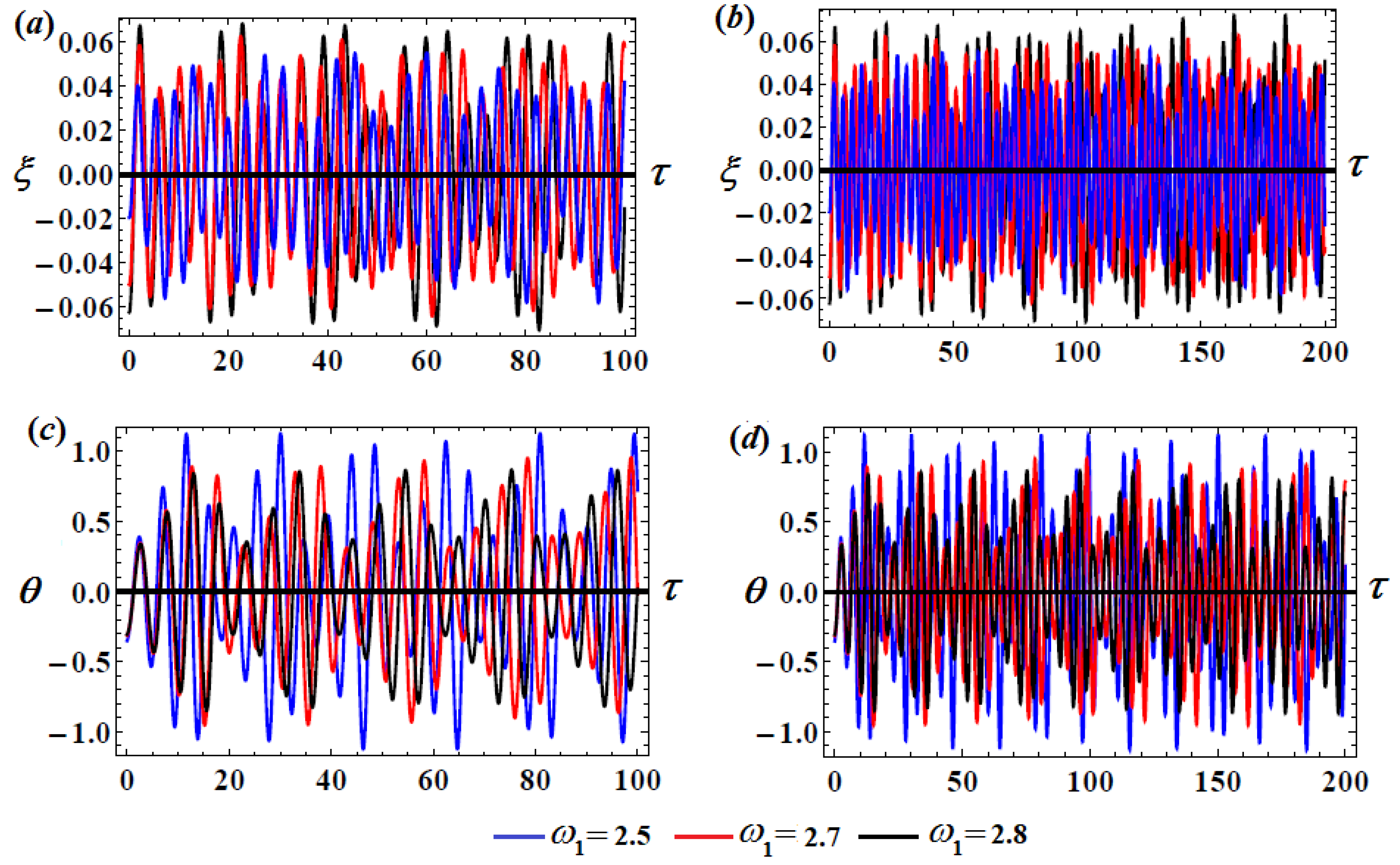
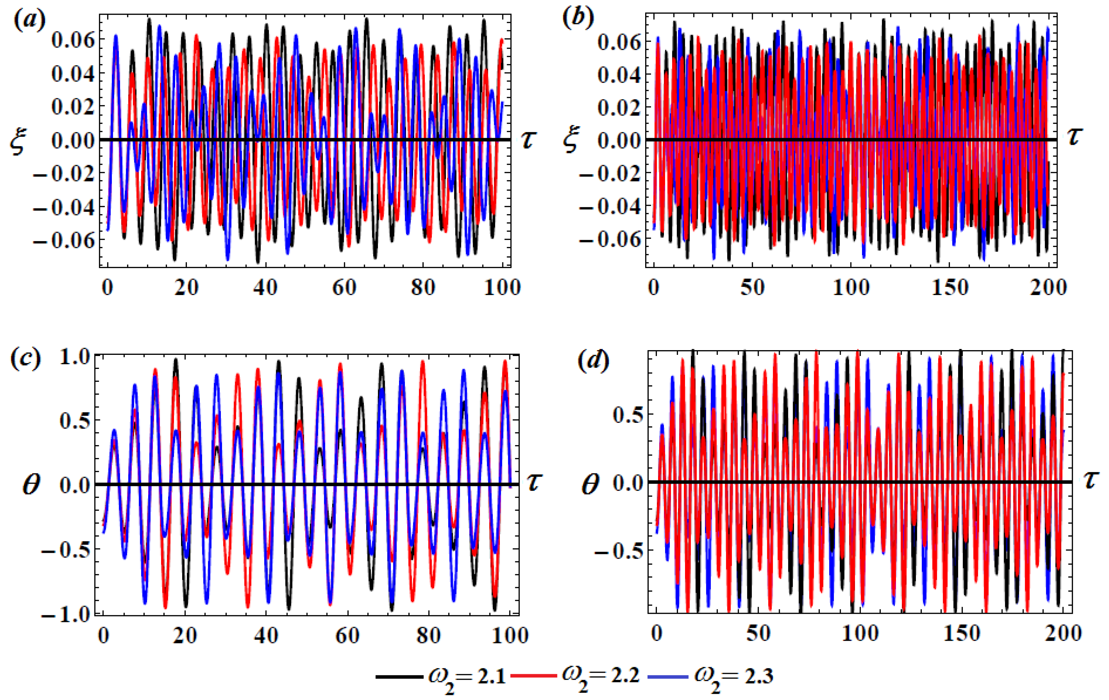
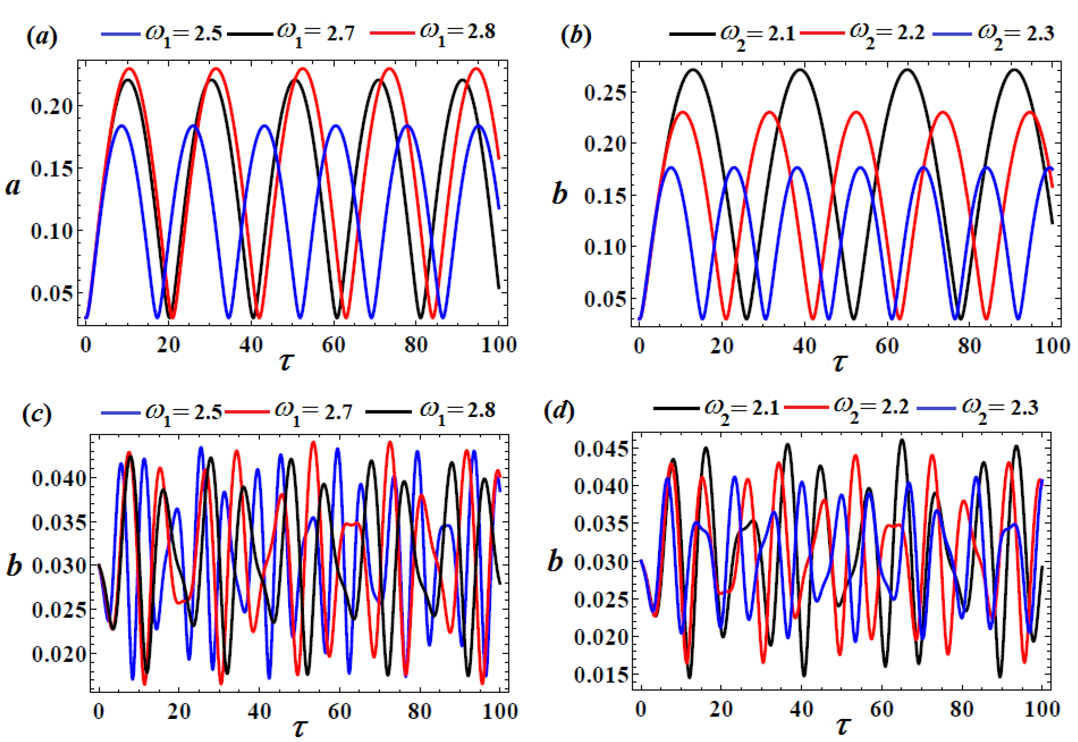
Parts of Figure 2 represent the variation of the solutions $\xi$ and $\theta$ via $\tau$ during the specified time intervals $[0,100] \mathrm{s}$ and $[0,200] \mathrm{s}$. These figures are calculated when ${\omega }_1$ takes the different values ${\omega }_1(=2.5,2.7,2.8) {\mathrm{s}}^{-1}$ at ${\omega }_2=2.1 {\mathrm{s}}^{-1},$ $c_1=0.02,c_2=0.03 {\mathrm{m}}^{-2}$. Figure 3 gives an indication of the behavior of the solutions $\xi$ and $\theta$ when ${\omega }_2=2.1 {\mathrm{s}}^{-1},{\omega }_2=2.2 {\mathrm{s}}^{-1},$ and ${\omega }_2=2.3 {\mathrm{s}}^{-1}$, with the same previous data of $c_1$ and $c_2$.

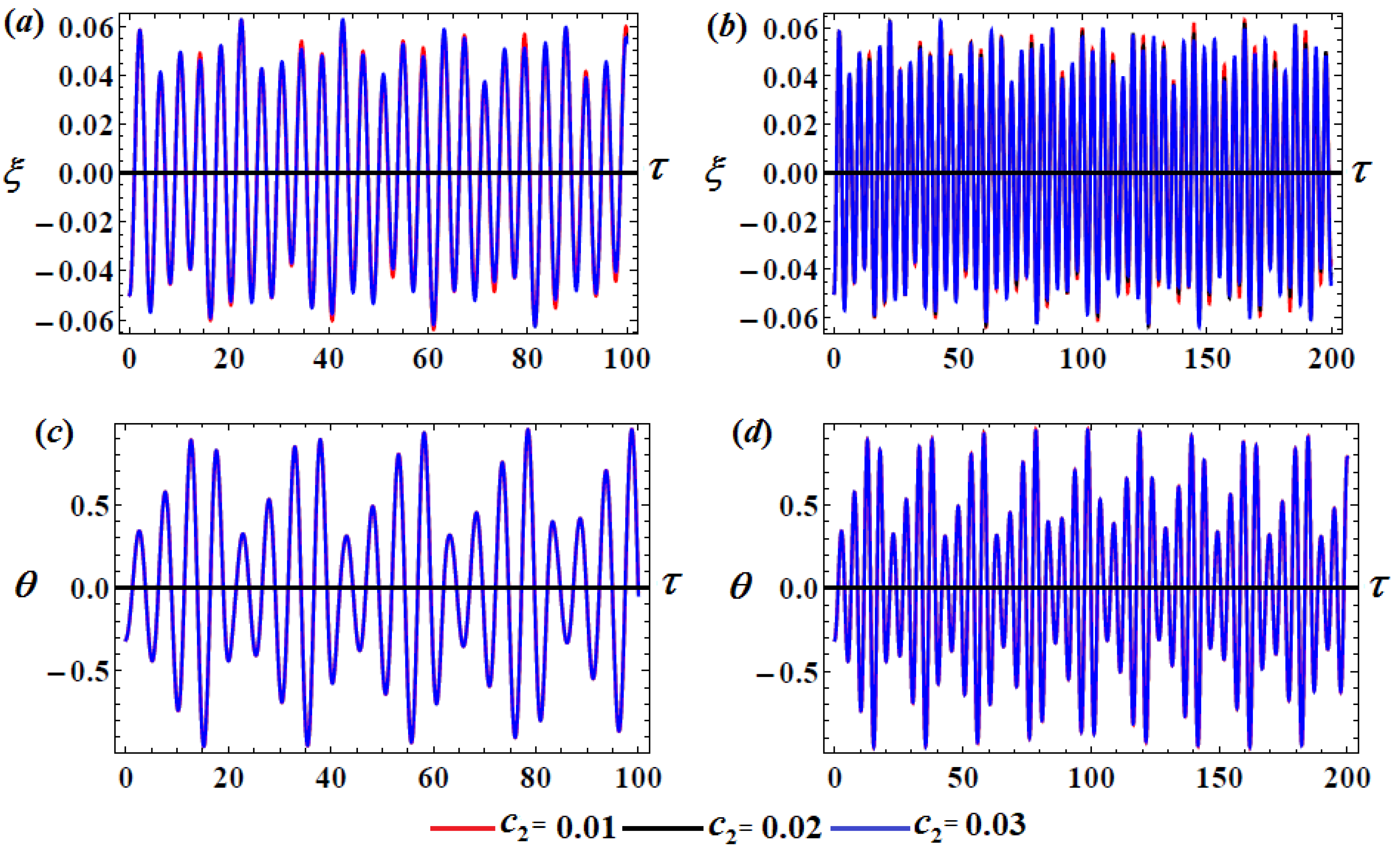
On the other side, the time histories that are reported in Figure 4 are computed when ${\omega }_2=2.2 {\mathrm{s}}^{-1}$ at different values of $c_1(=0.03,0.04,0.05)$ for the solutions $\xi$ and $\theta$. On the other hand, is based on calculations for different values of $c_2(=0.01,0.02,0.03) {\mathrm{m}}^{-2}$ for $\xi$ and $\theta$.

An inspection of Figure 2a shows that when ${\omega }_1$ increases from $2.5 s^{-1}$ to $2.8 s^{-1}$ with the constancy of the other parameters, periodic waves for the solution $\xi$ are obtained, and the number of oscillations decreases with the notable increment of the amplitudes. This means that through variation of time $\tau$ from $0$ to $100 \mathrm{s}$, the horizontal motion of mass $m$ is stable. On the other hand, the behavior of $\theta$ has a periodic form during the same time interval, and there is a slight variation of the amplitude; see part (c) of the same figure. This conclusion encourages us to expand the interval time of motion to $[0,200] \mathrm{s}$, as seen in parts (b) and (d) for the elongation $\xi$ and the rotating angle $\theta$, respectively. The waves included in part (b) behave as a periodic form, with the tendency to decrease the amplitude along the considered time interval, while the manner of $\theta$ has decay behavior, as is obvious from part (d).

The time histories reported in Figure 3 for the solutions $\xi$ and $\theta$ are computed when ${\omega }_2$ has different values, and they are plotted when $\tau \in [0,100] \mathrm{s}$ and $\tau \in [0,200] \mathrm{s}$. Similarly, it is obvious that the behavior of the attained waves varies between periodicity and decay. By focusing on parts (a) and (c) of Figure 3, it is clear that when ${\omega }_2$ increases, the number of oscillations increases and their amplitudes decrease. On the other side, the number of fluctuations has the same behavior, with the increasing of the amplitude as illustrated in part (b) of Figure 3. The plots included in part (d) of the same figure reveal that when ${\omega }_2$ increases, the steadiness of the amplitude (to some extent) during the considered time interval $\theta$ is observed. Therefore, the investigated motion is stable. On the other side, the variation of $\xi$ via $\tau$ when $c_1$ has distinct values is plotted in Figure 4, in which the impact of different values of $c_1$ becomes slight for the waves that describe $\xi$, as indicated in parts (a) and (b), while there is no significant change of $\theta$ waves, as seen in parts (c) and (d) of the same figure.

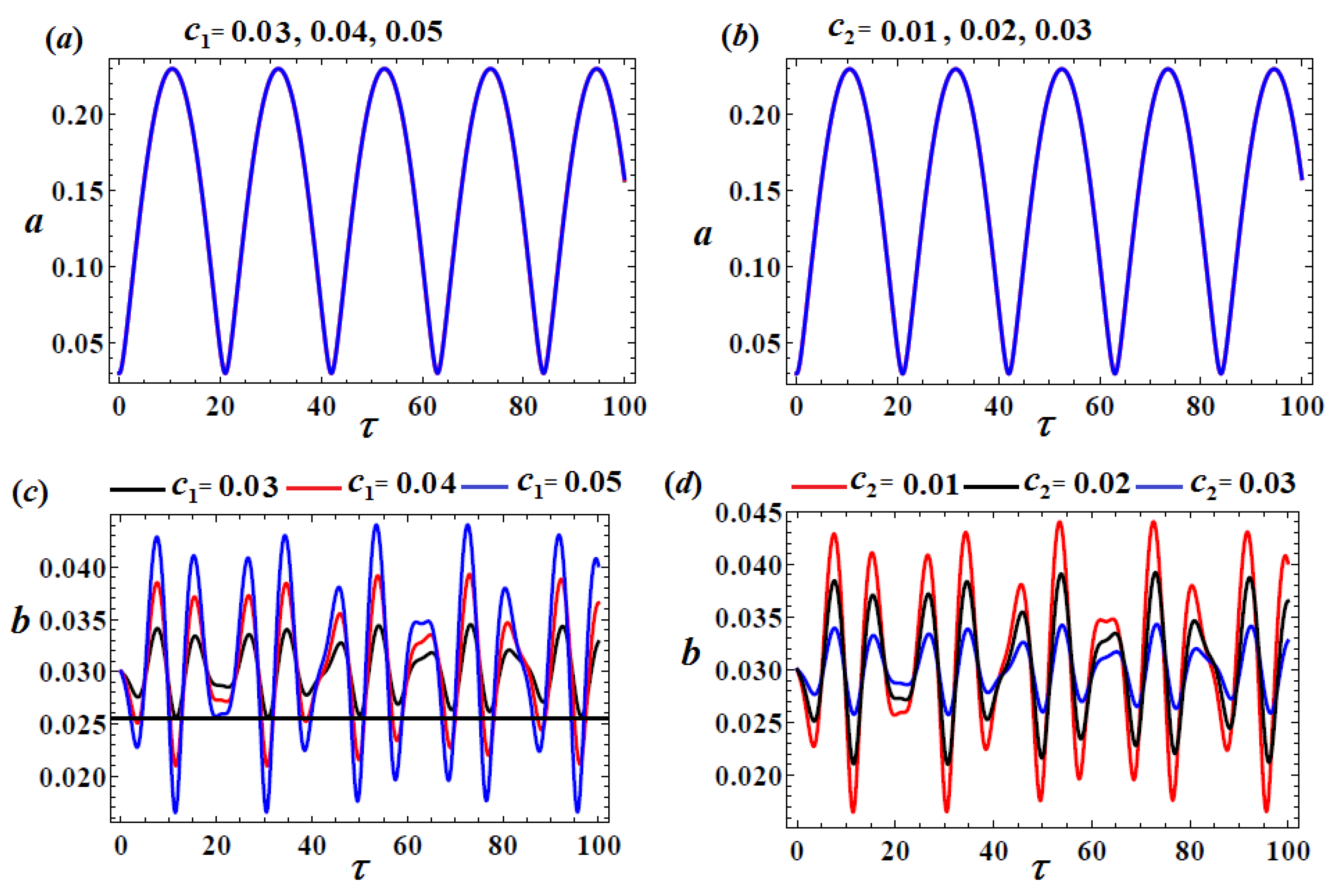
According to the calculations depicted in Figure 5, we conclude that with the shift of values of $c_2$ from $0.01$ to $0.03$ through the value $0.02$, there is a slight variation of the observed elongation waves. However, there is no variation of the rotating angle $\theta$, as Equation (35) does not depend on $c_2$, while Equation (37) depends directly on the same parameter.

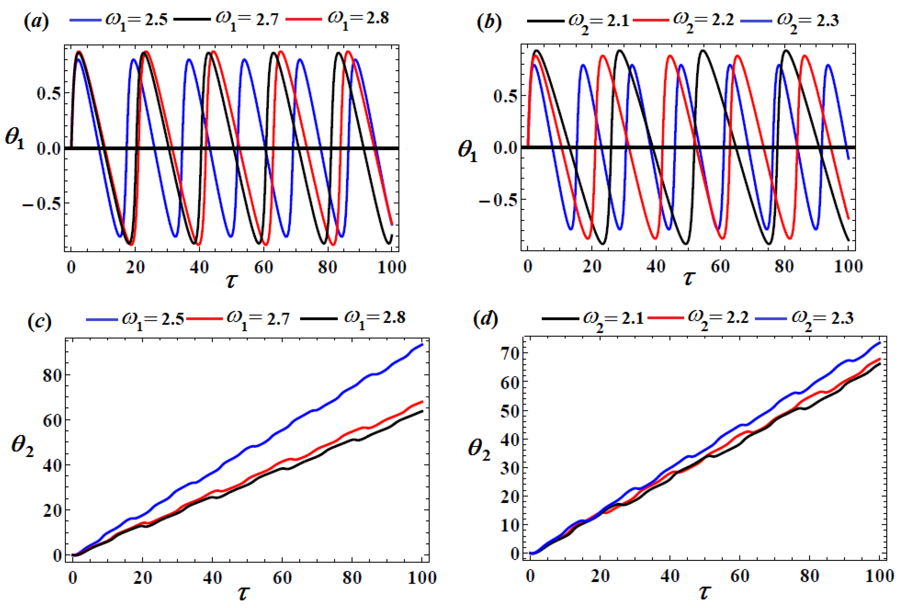
After grasping the previous analysis, we investigate the behavior of the phases and amplitudes of the achieved solutions when one of the parameters ${\omega }_1$ or $c_j (j=1,2)$ changes with the constancy of the others. Therefore, it should be noted that when ${\omega }_1$ and ${\omega }_2$ have different values, we notice a fluctuating effect on the amplitude $a$ of the horizontal elongation $\xi$, as observed in parts (a) and (b) of Figure 6, while the amplitude $b$ of the rotating angle $\theta$ fluctuated during the considered time interval according to the values of ${\omega }_1$ and ${\omega }_2$, as in parts (c) and (d), respectively. Moreover, the corresponding phases ${\theta }_1$ have excellent impact, as specified in parts (a) and (b) of Figure 7, due to the variations of ${\omega }_1$ and ${\omega }_2$, respectively. On the other side, the impact of ${\omega }_1$ and ${\omega }_2$ on the waves reveals a sharp increment in ${\theta }_2$ behavior, as seen from Figure 7c,d.

Another concrete example involves the variations of $a,b,$ and ${\theta }_j (j=1,2)$ according to different values of $c_j$. The corresponding plots are included in Figure 8 and Figure 9. The amplitude $a$ does not vary with $c_j$ as well as ${\theta }_1$, which are portrayed in parts (a) and (b) of the same figures. Alternatively, the variation becomes clear with the amplitude $b$, while it becomes slight with the second phase ${\theta }_2$.

Based on this discussion, we conclude that the model’s motion is stable and chaos-free.

6. Analysis of the Stability

The Routh-Hurwitz approach to the non-linear stability [37] is used in this section to explore the stability of the investigated auto-parametric system. A damped spring and the external force have a good impact on the behavior of this system. Therefore, in addition to the simulations of the system’s non-linear evolution, the stability requirements are applied. It is found that the frequency $\omega$ and the damping coefficient $c_1$ play a significant role in these requirements.

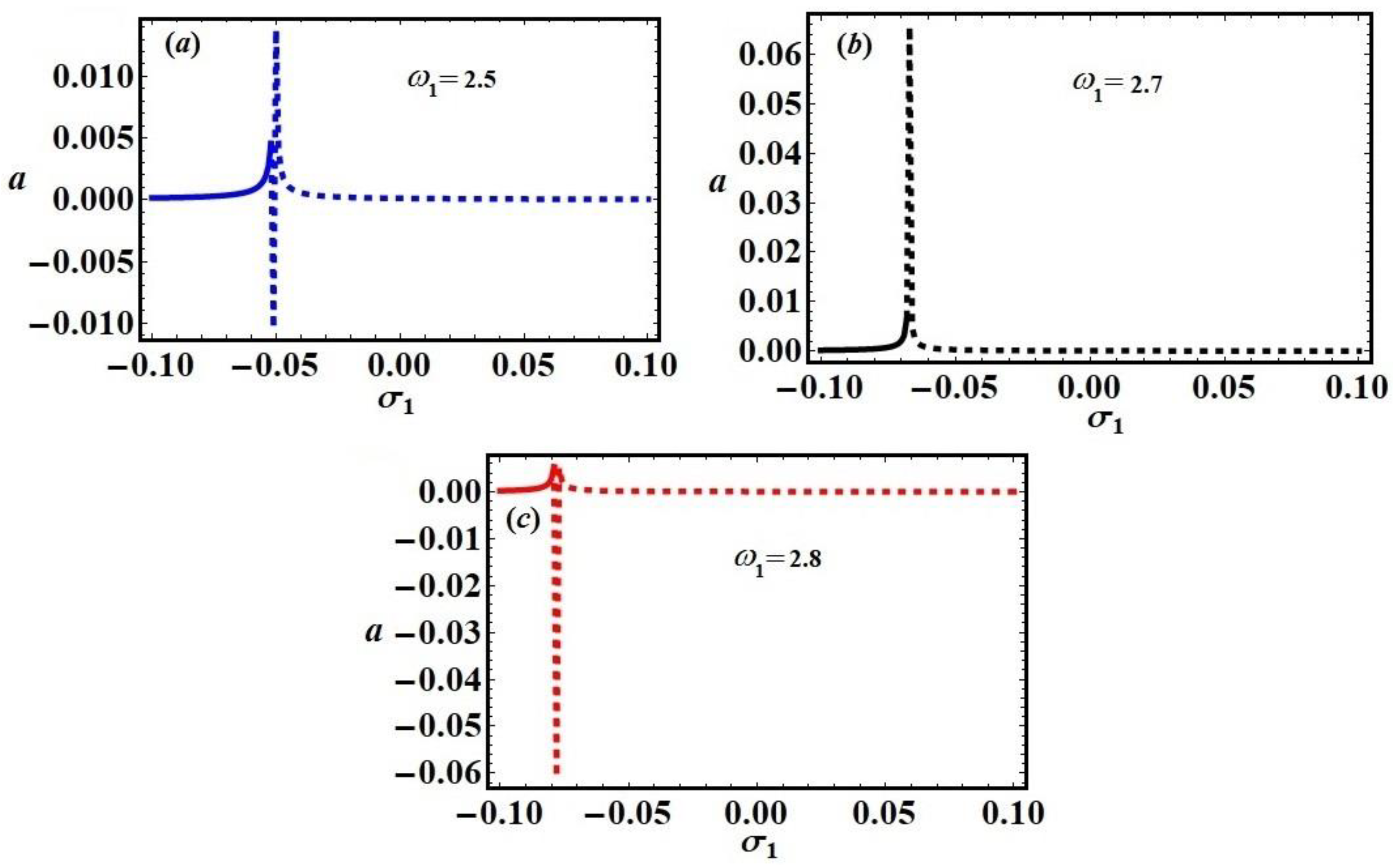
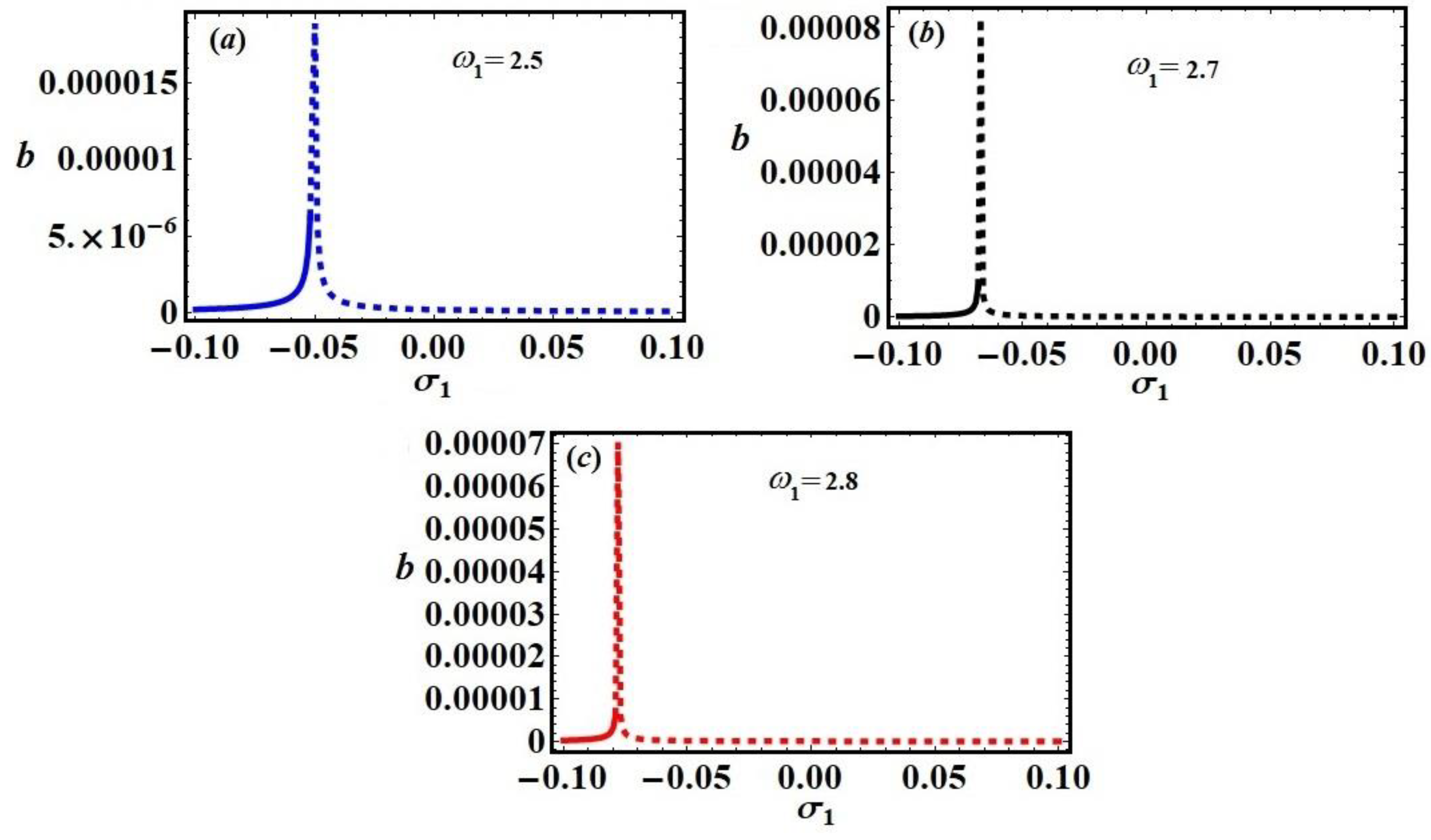
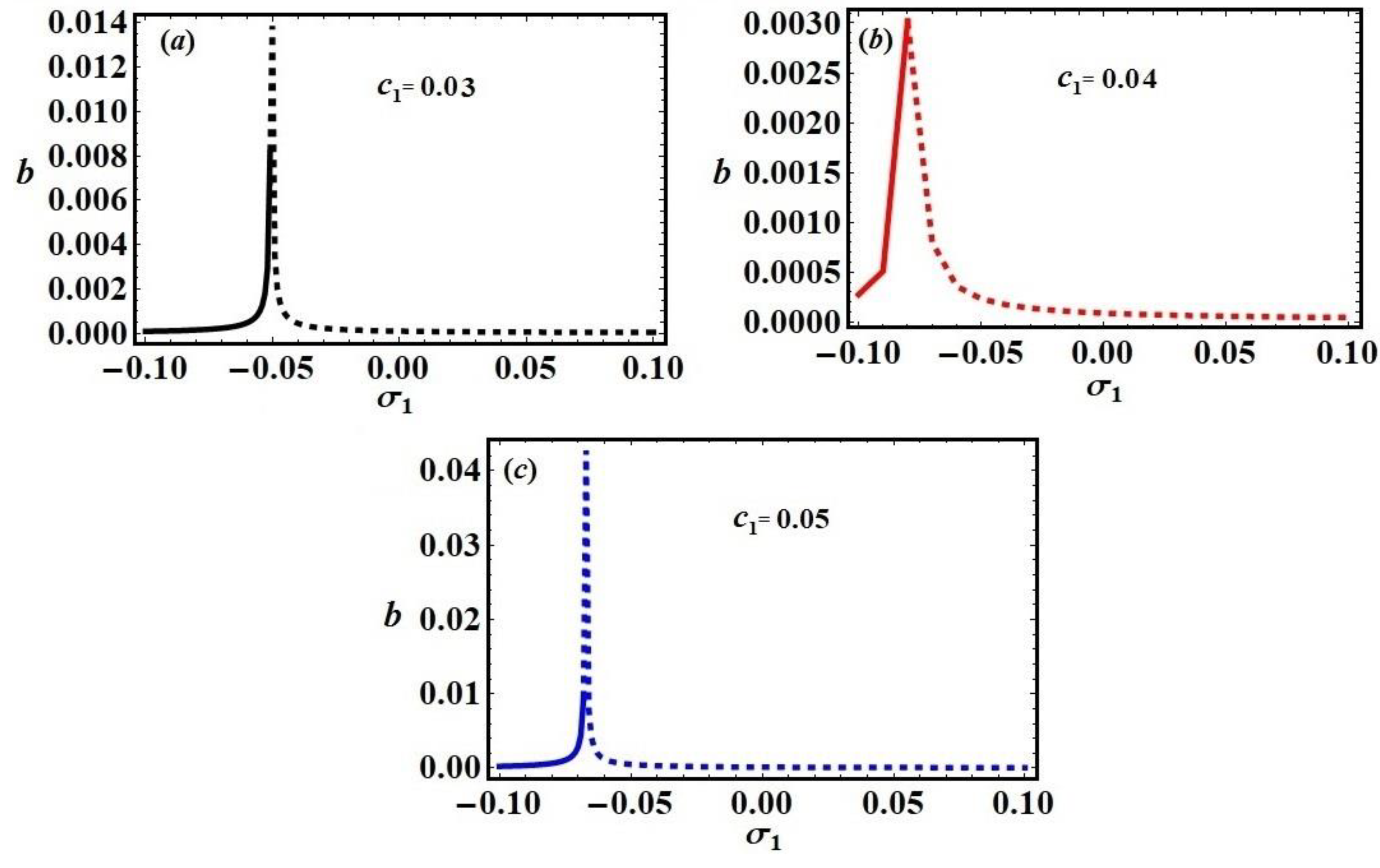
To achieve this purpose, system stability diagrams of the system of Equation (34) can be created using specific activity with different values of the system’s parameters. The variation of the modified amplitudes $a$ and $b$ are plotted versus the detuning parameter ${\sigma }_1$ in Figure 10, Figure 11, Figure 12 and Figure 13 to reveal the stability and instability zones of the possible fixed points and to show the frequency response curves at different values of $\omega$ and $c_1$ in which the solid curves describe the stable ranges of fixed points, while the dashed curves show the unstable ranges.

Figure 10 and Figure 11 show the influence of ${\sigma }_1$ on the frequency response curve at $c_1=0.03,$ ${\sigma }_2=0.003,$ and ${\omega }_1(=2.5,2.7,2.8)$, in which the stable and unstable areas of fixed points for the distinct values of ${\omega }_1$, as seen in both figures, are $-0.1\le {\sigma }_1\le -0.052,$$-0.1\le {\sigma }_1\le -0.068,$$-0.1\le {\sigma }_1\le -0.079$ and $-0.052<{\sigma }_1\le 0.1,$$-0.068<{\sigma }_1\le -0.1,$$-0.079<{\sigma }_1\le 0.1$, respectively. Figure 12 and Figure 13 present the frequency response curves when ${\omega }_1=2.5,$ ${\sigma }_2=0.003$ and $c_1(=0.03,0.04,0.05)$ for the amplitudes $a$ and $b$ via the detuning parameter ${\sigma }_1$. It is notable that there are different ranges of stability and instability areas for the mentioned values of the damped coefficient $c_1$. These ranges can be classified according to the following values: the stability areas at $c_1=0.03,$ $c_1=0.04,$ and $c_1=0.05$ are $-0.1\le {\sigma }_1\le -0.051,$$-0.1\le {\sigma }_1\le -0.08,$ and $-0.1\le {\sigma }_1\le -0.098$, respectively. The instability areas at the same values of $c_1$ are $-0.051<{\sigma }_1\le 0.1,$$-0.08<{\sigma }_1\le 0.1,$ and $-0.098<{\sigma }_1\le 0.1$.

It is observed that there is a high resonance between the frequencies in the range $-0.1\le {\sigma }_1\le 0.1$ of the examined areas, which leads to a significant rise in the amplitudes of the steady-state solutions.

7. Concluding Remarks

The motion of the 2DOF auto-parametric pendulum model consisting of a mass $M$ attached to a damped spring and connected with a rotating rigid arm (of mass $m$ and length $\mathrm{l}$) under the action of an external force on the other end of the arm was studied. The governing EOM were obtained utilizing Lagrange’s equations. The MMS was used to achieve the second-order approximate solutions of these equations and to locate the resonances of the system. The cases of simultaneously primary external and internal resonances were examined. The modulation equations were developed in the framework of the solvability conditions. The variables of phase and amplitude were used to study the solutions at the steady state. The requirement of stability of the steady-state solutions was obtained using the Routh-Hurwitz criterion. The portrayal representation of the time histories of the acquired solutions was used to evaluate the influence of various parameters on the dynamical behavior of the considered model. The stability and instability zones of the system were explored, in which it was shown that the system’s performance was stable for some of its variables. The acquired results are more consistent with those obtained in [15] (in the absence of both the pendulum and the acting force on the dynamic model), indicating that the current study should be viewed as a generalization of past work while asserting the novelty of the investigated model and the obtained results. The obtained results can be applied to the vibration damping of many mechanical areas, both linear and angular.

References

- Yu, T.-J.; Zhang, W.; Yang, X.-D. Global dynamics of an autoparametric beam structure. Nonlinear Dyn. 2017, 88, 1329–1343. [Google Scholar] [CrossRef]
- Ikeda, T. Nonlinear parametric vibrations of an elastic structure with a rectangular liquid tank. Nonlinear Dyn. 2003, 33, 43–70. [Google Scholar] [CrossRef]
- Cveticanin, L.; Zukovic, M.; Cveticanin, D. Oscillator with variable mass excited with non-ideal source. Nonlinear Dyn. 2018, 92, 673–682. [Google Scholar] [CrossRef]
- Cartmell, M.C. Introduction to Linear, Parametric and Non-Linear Vibrations; Springer Science & Business Media: Berlin/Heidelberg, Germany, 1990. [Google Scholar]
- Nayfeh, A.H.; Mook, D.T. Nonlinear Oscillations; Wiley-VCH: Weinheim, Germany, 2004. [Google Scholar]
- Fossen, T.I.; Nijmeijer, H. Parametric Resonance in Dynamical Systems; Springer Science & Business Media: Berlin/Heidelberg, Germany, 2012. [Google Scholar]
- Zhu, S.J.; Zheng, Y.F.; Fu, Y.M. Analysis of non-linear dynamics of a two-degree-of-freedom vibration system with non-linear damping and non-linear spring. J. Sound Vib. 2004, 271, 15–24. [Google Scholar] [CrossRef]
- El Rifai, K.; Haller, G.; Bajaj, A.K. Global dynamics of an autoparametric spring-mass-pendulum system. Nonlinear Dyn. 2007, 49, 105–116. [Google Scholar] [CrossRef] [Green Version]
- Kecik, K.; Warminski, J. Dynamics of an autoparametric pendulum-like system with a nonlinear semiactive suspension. Math. Probl. Eng. 2011, 2011, 451047. [Google Scholar] [CrossRef] [Green Version]
- Kecik, K.; Mitura, A.; Warmiński, J. Efficiency analysis of an autoparametric pendulum vibration absorber. Eksploat. Niezawodn. 2013, 15, 221–224. [Google Scholar]
- Baleanu, D.; Asad, J.H.; Jajarmi, A. New aspects of the motion of a particle in a circular cavity. In Proceedings of the Romanian Academy, Series A—Mathematics Physics Technical Sciences Information Science; Publishing House of the Romanian Academy: Bucharest, Romania, 2018; Volume 19, pp. 361–367. [Google Scholar]
- Baleanu, D.; Jajarmi, A.; Asad, J.H. Classical and fractional aspects of two coupled pendulums. Rom. Rep. Phys. 2019, 71, 103. [Google Scholar]
- Baleanu, D.; Sajjadi, S.S.; Jajarmi, A.; Asad, J.H. New features of the fractional Euler-Lagrange equations for a physical system within non-singular derivative operator. Eur. Phys. J. Plus 2019, 134, 181. [Google Scholar] [CrossRef]
- Baleanu, D.; Asad, J.H.; Jajarmi, A. The fractional model of spring pendulum: New features within different kernels. In The Romanian Academy Series A—Mathematics Physics Technical Sciences Information Science; Publishing House of the Romanian Academy: Bucharest, Romania, 2018; Volume 19, pp. 447–454. [Google Scholar]
- Vazquez-Gonzalez, B.; Silva-Navarro, G. Evaluation of the autoparametric pendulum vibration absorber for a Duffing system. Shock. Vib. 2008, 15, 355–368. [Google Scholar] [CrossRef] [Green Version]
- Khirallah, K. Autoparametric amplification of two nonlinear coupled mass-spring systems. Nonlinear Dyn. 2018, 92, 463–477. [Google Scholar] [CrossRef]
- Nabergoj, R.; Tondl, A.; Virag, Z. Autoparametric resonance in an externally excited system. Chaos Solitons Fract. 1994, 4, 263–273. [Google Scholar] [CrossRef]
- Kamel, M. Bifurcation analysis of a nonlinear coupled pitch-roll ship. Math. Comput. Simul. 2007, 73, 300–308. [Google Scholar] [CrossRef]
- Zhou, L.; Chen, F. Stability and bifurcation analysis for a model of a nonlinear coupled pitch-roll ship. Math. Comput. Simul. 2008, 79, 149–166. [Google Scholar] [CrossRef]
- Amer, T.S.; Bek, M.A. Chaotic responses of a harmonically excited spring pendulum moving in circular path. Nonlinear Anal. RWA 2009, 10, 3196–3202. [Google Scholar] [CrossRef]
- Moore, H. Matlab for Engineers, 3rd ed.; Pearson: London, UK, 2012. [Google Scholar]
- Amer, T.S. The dynamical behavior of a rigid body relative equilibrium position. Adv. Math. Phys. 2017, 2017, 8070525. [Google Scholar] [CrossRef]
- Amer, T.S.; Bek, M.A.; Hamada, I.S. On the motion of harmonically excited spring pendulum in elliptic path near resonances. Adv. Math. Phys. 2016, 2016, 8734360. [Google Scholar] [CrossRef] [Green Version]
- Amer, T.S.; Bek, M.A.; Abouhmr, M.K. On the vibrational analysis for the motion of a harmonically damped rigid body pendulum. Nonlinear Dyn. 2018, 91, 2485–2502. [Google Scholar] [CrossRef]
- El-Sabaa, F.M.; Amer, T.S.; Gad, H.M.; Bek, M.A. On the motion of a damped rigid body near resonances under the influence of harmonically external force and moments. Results Phys. 2020, 19, 103352. [Google Scholar] [CrossRef]
- Bek, M.A.; Amer, T.S.; Sirwah, M.A.; Awrejcewicz, J.; Arab, A.A. The vibrational motion of a spring pendulum in a fluid flow. Results Phys. 2020, 19, 103465. [Google Scholar] [CrossRef]
- Meirovitch, L. Fundamental of Vibrations; McGraw-Hill: New York, NY, USA, 2001. [Google Scholar]
- Nagashima, I. Optimal displacement feedback control law for active tuned mass damper. Earthq. Eng. Struct. Dyn. 2001, 30, 1221–1242. [Google Scholar] [CrossRef]
- Eissa, M.; Sayed, M. A comparison between active and passive vibration control of non-linear simple pendulum, part I: Transversally tuned absorber and negative feedback. Math. Comput. Appl. 2006, 11, 137–149. [Google Scholar] [CrossRef] [Green Version]
- Eissa, M.; Sayed, M. A Comparison between active and passive vibration control of non-linear simple pendulum, part II: Longitudinal tuned absorber and negative and feedback. Math. Comput. Appl. 2006, 11, 151–162. [Google Scholar] [CrossRef] [Green Version]
- Eissa, M. Vibration reduction of a three DOF non-linear spring pendulum. Commun. Nonlinear Sci. Numer. Simul. 2008, 13, 465–488. [Google Scholar] [CrossRef]
- Amer, T.S.; Bek, M.A.; Hassan, S.S. The dynamical analysis for the motion of a harmonically two degrees of freedom damped spring pendulum in an elliptic trajectory. Alex. Eng. J. 2022, 61, 1715–1733. [Google Scholar] [CrossRef]
- Abady, I.M.; Amer, T.S.; Gad, H.M.; Bek, M.A. The asymptotic analysis and stability of 3DOF non-linear damped rigid body pendulum near resonance. Ain Shams Eng. J. 2021, in press. [Google Scholar] [CrossRef]
- Gilat, A. Numerical Methods for Engineers and Scientists; Wiley: Hoboken, NJ, USA, 2013. [Google Scholar]
- Tewari, A. Modern Control Design with Matlab and Similink; John Wiley and Sons Ltd.: New York, NY, USA, 2002. [Google Scholar]
- Abohamer, M.K.; Awrejcewicz, J.; Starosta, R.; Amer, T.S.; Bek, M.A. Influence of the motion of a spring pendulum on energy-harvesting devices. Appl. Sci. 2021, 11, 8658. [Google Scholar] [CrossRef]
- Amer, T.S.; Starosta, R.; Elameer, A.S.; Bek, M.A. Analyzing the stability for the motion of an unstretched double pendulum near resonance. Appl. Sci. 2021, 11, 9520. [Google Scholar] [CrossRef]
Figure 1.
Dynamical model.
Figure 2.
Time history portraits of and when and : (a,c) during the time interval and (b,d) during the time interval .
Figure 3.
Figure 4.
Impact of on the behavior of and : (a,c) during the time interval and (b,d) during the time interval .
Figure 5.
Impact of on the behavior of and : (a,c) at and (b,d) at .
Figure 6.
Behavior of the amplitudes and with regard to the horizontal elongation and the rotation angle respectively: (a,c) at and (b,d) at .
Figure 7.
Behavior of the phase angles and concerning the horizontal elongation and the rotation angle respectively: (a,c) for different values of and (b,d) for different values of .
Figure 8.
(a,c) The effect of and (b,d) the effect of on the amplitudes and with regard to the horizontal elongation and the rotation angle , respectively.
Figure 9.
(a,c) The effect of and (b,d) the effect of on the phases and with regard to the horizontal elongation and the rotation angle , respectively.
Figure 10.
Frequency response of the amplitude at : (a) (b) (c) .
Figure 11.
Frequency response curves of the amplitude at : (a) (b) (c) .
Figure 12.
Frequency response curves of at : (a) (b) (c) .
Figure 13.
Publisher’s Note: MDPI stays neutral with regard to jurisdictional claims in published maps and institutional affiliations. |
© 2021 by the authors. Licensee MDPI, Basel, Switzerland. This article is an open access article distributed under the terms and conditions of the Creative Commons Attribution (CC BY) license (https://creativecommons.org/licenses/by/4.0/).
Share and Cite
MDPI and ACS Style
Amer, W.S.; Amer, T.S.; Starosta, R.; Bek, M.A. Resonance in the Cart-Pendulum System—An Asymptotic Approach. Appl. Sci. 2021, 11, 11567. https://0-doi-org.brum.beds.ac.uk/10.3390/app112311567
AMA Style
Amer WS, Amer TS, Starosta R, Bek MA. Resonance in the Cart-Pendulum System—An Asymptotic Approach. Applied Sciences. 2021; 11(23):11567. https://0-doi-org.brum.beds.ac.uk/10.3390/app112311567
Chicago/Turabian StyleAmer, Wael S., Tarek S. Amer, Roman Starosta, and Mohamed A. Bek. 2021. "Resonance in the Cart-Pendulum System—An Asymptotic Approach" Applied Sciences 11, no. 23: 11567. https://0-doi-org.brum.beds.ac.uk/10.3390/app112311567
Note that from the first issue of 2016, this journal uses article numbers instead of page numbers. See further details here.