
Force Measurement with a Strain Gauge Subjected to Pure Bending in the Fluid–Wall Interaction of Open Water Channels


1
Department of Civil and Environmental Engineering, Universidad del Bío-Bío, Concepción 4081112, Chile
2
Department of Water Resources, College of Agricultural Engineering, Universidad de Concepción, Chillán 3812120, Chile
3
Centro de Investigación en Sustentabilidad y Gestión Energética de Recursos (CiSGER), School of Engineering, Universidad del Desarrollo, Las Condes 7610658, Chile
*
Author to whom correspondence should be addressed.
Appl. Sci. 2022, 12(3), 1744; https://0-doi-org.brum.beds.ac.uk/10.3390/app12031744
Submission received: 29 October 2021
/
Revised: 21 January 2022
/
Accepted: 21 January 2022
/
Published: 8 February 2022
(This article belongs to the Special Issue Non-destructive Testing in Civil Engineering)
Abstract
:Featured Application
This research has specific applications in the measurement of forces of small magnitude, which occur in the fluid–wall interaction, through a non-destructive technique that allows for measuring the shear stress in open water channels.
Abstract
An experimental method to measure forces of small magnitude with a strain gauge as a force sensor in the fluid–wall interaction of open water channels is presented. Six uniaxial strain gauges were employed for this purpose, which were embedded across the entire sensing area and subjected to pure bending, employing two-point bending tests. Sixteen two-point bending tests were performed to determine the existence of a direct relationship between the load and the instrument signal. Furthermore, a regression analysis was used to estimate the parameters of the model. A data acquisition system was developed to register the behavior of the strain gauge relative to the lateral displacement induced by the loading nose of the universal testing machine. The results showed a significant linear relationship between the load and the instrumental signal, provided that the strain gauge was embedded between 30% and 45% of the central axis in the sensing area of the sensor (R2 > 0.99). Thus, the proposed sensor can be employed to measure forces of small magnitude. Additionally, the linear relationship between the load and the instrumental signal can be used as a calibration equation, provided that the strain gauge is embedded close to the central axis of the sensing area.
1. Introduction
The direct measurement of small forces has shown to have great practical significance in many fields such as sciences, engineering, the industrial sector, and medicine—among many others—and its relevance was first recognized in the 1970s [1], continuing its growth to this day.
One of the applications of measurement of small forces can be found when studying the fluid–wall interaction of open water channels. In this sense, shear stress in open water channels—the action exerted by water on the channel bed material—can alter the state of rest or movement of the bed material, either by sedimentation, dragging, scour, or transport of the material. Wall–water stores oppose the movement of the fluid and affect the flow velocity profile. Drag and shear stress due to vegetation reduce flow discharge in channels, but they also allow flood attenuation and sediment deposition [2,3]. Shear stress, dragging, and sediment transport have been widely studied, and there exist limitations on using conventional formulas, such as the Manning equation [2]. Average bed shear stress is difficult to derive from the bulk flow characteristics, such as applying predefined velocity profiles or the shear stress distribution. Currently, there is a wide range of methods for direct and indirect measurement of shear stress in open channels. However, direct measurements of shear stress in the wall–fluid interface are less frequent. Tinoco et al. [4] classify intrusive approaches (acoustic Doppler velocimeters, optical backscatter sensors, ultrasonic velocity profilers, and acoustic Doppler current profilers) and non-intrusive techniques (laser-induced fluorescence, particle image velocimetry, and laser Doppler velocimetry) to detect the magnitude of the flow disturbance by the experimental probe itself. Detailed reviews about methods to measure and estimate shear stress can be found in Huai et al. [5]. Experimental setups range from large-scale measurements (e.g., Errico et al. [6]) to highly controlled laboratory-based experiments (e.g., Duan et al. [7] and Bashirzadeh et al. [8]). The direct measurement of shear stress requires sensitivity to small changes in flow velocity, generates minimal flow disturbance, especially in the vicinity of the bed, and maintains the principle of no sliding of the material in the bed [9,10,11].
The development of microsystems, nanotechnology, fluid dynamics, aerodynamics, biotechnology, and biomedical technology, among others, involves the application of devices suitable to measure forces from the force scale of millinewtons (mN) to micronewtons (µN). On one side, microelectromechanical sensors (MEMS) such as systems based on interferometry, oil films, and liquid crystal coatings have shown improvements in performance and accuracy relative to conventional techniques (hybrid MEMS) and have been used to measure skin friction [12]. On the other hand, multidimensional F/M MEMS are used to measure force and moment in robotics, electronics, and the development of medical equipment and smart devices [1].
The techniques employed for these measurements can be direct or indirect [13,14]. Despite the usefulness of these sophisticated devices to measure forces induced by external loads, they are limited by their complex calibration and testing procedures, which are not sufficiently structured because of the miniaturization of sensors [12,13,14,15,16].
Electrical resistance strain gauges are one of the simplest and most frequently used passive transducers. They are usually bonded to one of the surfaces of the specimen to be tested to generate only axial tension and compression. They have been used as load or strain transducers of sophisticated devices since their manufacturing technology and encapsulation prevent them from suffering mechanical and environmental damage. Due to their small size, sensitivity, accuracy, simplicity, and low cost compared to sophisticated devices, strain gauges are broadly used in laboratories worldwide as sensing devices [16]. Nonetheless, no research has been found that explores the operating principle of strain gauges subjected to pure bending. This is because the bending effect is considered negligible concerning the tension–compression effect. In the fields of fluid dynamics and aerodynamics, the measurement of small forces involved in the fluid–wall interaction is required to analyze the stability of walls and fluids.
Consequently, there is a lack of simple devices for measuring forces of small magnitude, in the order of mN, that can be employed to measure flows of water in open and closed systems. Due to the foregoing, the strain gauge is proposed to be used as a device for measuring small forces, used in a way different from that for which it was designed; that is to say, the strain gauge itself is subjected to pure bending. Furthermore, lateral displacement employing a two-point bending test (cantilever) induced in a way different from that defined by ASTM D747 [17] is proposed.
The proposed method is justified for the following reasons: Firstly, the size of the proposed device is in the order of millimeters. Therefore, it is smaller than the minimum dimensions required for standardized tests [17]. Secondly, in this type of test, the data analysis is based on the conventional beam theory [18], or the elastic theory [19], provided that there is a direct relationship between the applied load and the resultant lateral displacement within the elastic range of the specimen’s material. However, the appropriateness of the conventional beam theory for determining the relationship between the load and lateral displacement of a sample is called into question when the dimensions of the specimen are in the order of millimeters; thus, uncertainties are generated in the bending tests. Thirdly, because the geometric dimensions of the proposed device correspond to the ones of a small plate, it is difficult to obtain an analytical relationship between load and displacement. The numerical solutions (finite elements or differences) and analytical solutions (superposition method or integral transform method) [20] are well known; however, they require complex and time-consuming procedures. Furthermore, thin flats behave differently from beams in terms of strain and internal stress distribution, which is under Love–Kirchhoff’s theory.
For these reasons, the objective of this paper is to present the experimental results of two-point bending tests applied directly to strain gauges to measure forces of small magnitude directly. A direct relationship between the load and the instrumental signal is expected to be found because both of them depend on the lateral displacement of the device. Finally, these results are expected to be a practical contribution to the evidence about the mechanical behavior of strain gauges subjected to pure bending.
2. Materials and Methods
2.1. Materials and Experimental Setup
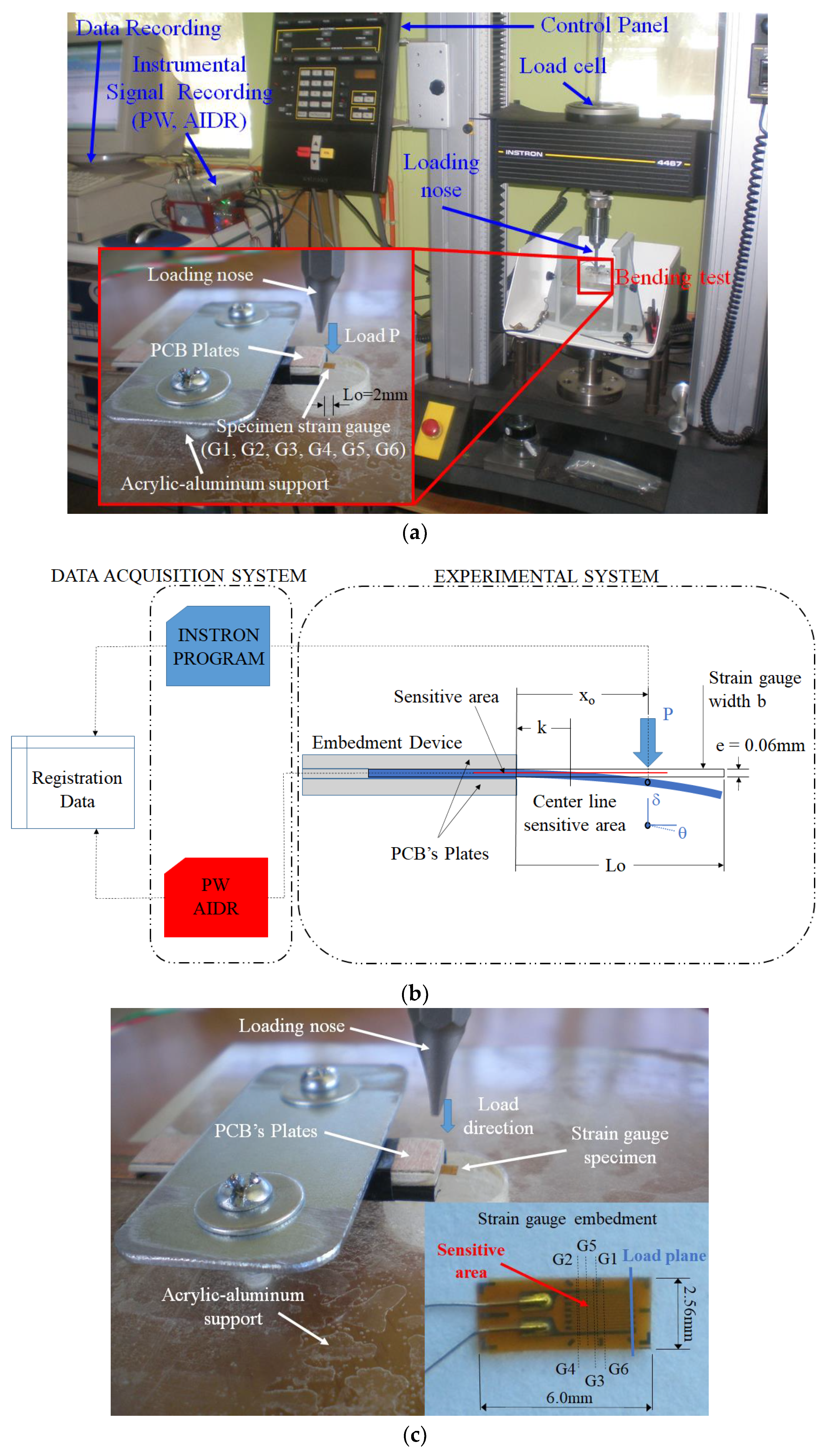
Figure 1 shows the experimental setup for the implementation of the proposed two-point bending test. Consequently, a total of sixteen two-point bending tests were carried out on the six strain gauges used as force sensors. The tests were carried out utilizing an INSTRON 4467 universal testing machine, which has a cell load of 10 N and a precision of 0.0025 N. Through the control panel and the software IX of the INSTRON, the geometric parameters and the characteristics of each test were defined. Furthermore, the reference values for force and displacement were established. All of the tests were performed at a constant speed of 1 mm/min, with a total displacement of the loading nose of 2 mm, which is in agreement with the ASAE Standard method S368.2 [21]. Simultaneously, the instrumental signal (indicated in Section 2.2) was recorded as a result of the data acquisition system, the devices developed, and the proposed strain gauge. In this sense, to subject the strain gauge to pure bending, each sensor was embedded within the sensing area employing two 3 mm thick printed circuit boards (PCB). Thus, these points are mentioned in Table 1, while the PCB plates were fitted to a 10-mm-thick acrylic plate (base of the materials testing machine) through an aluminum device as shown in Figure 1a,c.
In this study, six strain gauges (from G1 to G6 as shown in Figure 1a,c) used as force sensors were assessed. The strain gauges employed were simple, uniaxial, miniature strain gauges fabricated with copper-nickel alloy and completely coated with polyamide [22]. Their average geometric dimensions were 2.56 mm wide, 6.0 mm long and 0.06 mm thick, and their sensing area was 1.6 mm wide and 2.0 mm long, with a nominal resistance of 120Ω.
Table 1 shows the geometric dimensions and mechanical characteristics of the strain gauges used in the bending tests. Width (b), thickness (e), and the beam span (L0) were measured using a micrometer with a precision of 0.01 mm. The position of the loading nose concerning the embedment (xo) and the location of the embedment concerning the central axis of the sensing area (k) were measured using a Vernier caliper with a precision of 0.05 mm and verified using a photographic sample with a precision of 0.01 mm. The number of repetitions (R) was reduced to two due to the low coefficient of variation obtained for the G1 sensor, for which five repetitions were carried out. The tests, except that of the G6 sensor, were performed in a room with controlled temperature, as it is shown in Table 1. It has to be noted that the instrumental signals may be affected by temperature change; however, in this research, the temperature’s effect was not considered, since the calibration was carried out at a constant temperature in a controlled environment as previously mentioned.
The repeatability of the responses in the experimental tests was estimated for each sensor to analyze the validity of the data acquisition system and the universal testing machine. For each repetition, the beam span, the position, and the load speed of the loading nose remained constant. After finishing a test, the loading nose was returned to its initial position and the test was repeated.
2.2. Instrumental Signal Measurements in the Two-Point Bending Tests
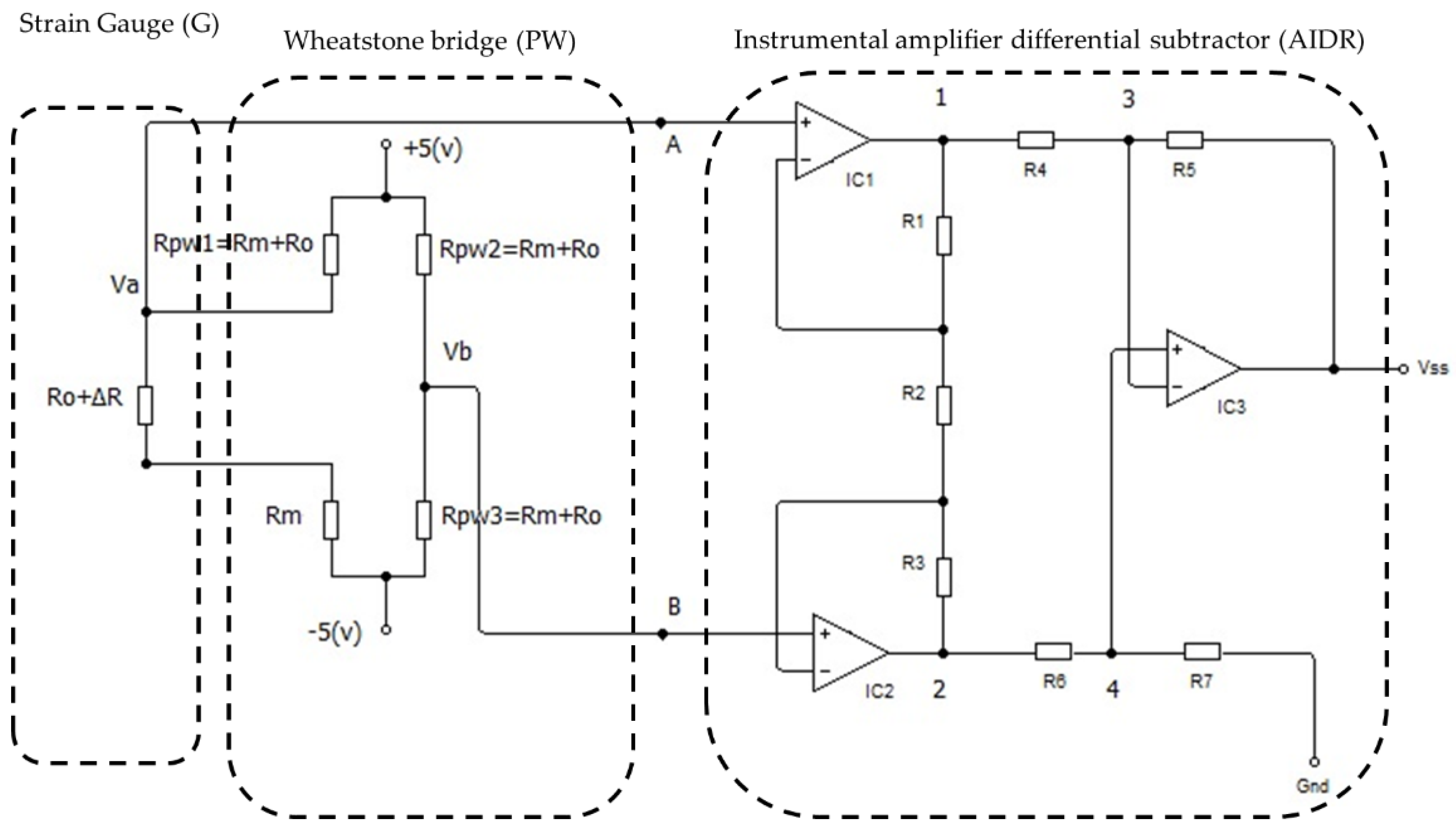
Figure 2 shows a scheme of the electronic circuits used to measure the instrumental signal in the two-point bending tests. The change in the electrical resistivity (ΔR) of the sensor when the strain gauge was being bent by the loading nose (see Figure 1b) was measured through a Wheatstone bridge (PW) because of its great precision [16,23]. As the signal (or drop in voltage) obtained from the PW was very small, in the range of millivolts, an instrumentation amplifier was required for the signal conditioning. In addition, a fixed-gain differential-input amplifier (AIDR) with high common-mode rejection was developed.
A Wheatstone bridge circuit (PW) in a quarter-bridge arrangement was used to register the changes in the electrical resistance of the sensor concerning its initial resistance (Ro). The quarter-bridge configuration was balanced (VAB = 0) and showed equality of nominal resistance values [8]. Moreover, an inactive gauge was added to prevent changes in resistance for the initial resistance. Resistors in series, Rm, were added to each component of the PW to establish a 10-mA upper limit for the current flow through the sensor. The resistor ratio Rm/Ro = 3.25 was employed for the resistors. In practice, the change in resistivity ΔR/Ro is in the range of 10−2, which is negligible relative to unity.
The response of the proposed device (sensor) was indicated in the PW through a voltage drop, as Equation (1) illustrates. This voltage drop and the change in resistivity of the sensor are in a proportional relationship because of the lateral displacement of the sensor. The constant of proportionality was 0.588.
The response of the sensor obtained by the PW is amplified by the AIDR circuit, wherein the voltage drops in nodes 3 and 4 must be the same (see Figure 2) to achieve a linear performance of the instrumentation amplifier. Therefore, the instrumental signal was obtained by applying Ohm’s law to each loop of the circuit shown in Figure 2, according to the output voltage given by Equation (2).
where and are the equivalent voltage drop percentages in terminals A and B of the Wheatstone bridge, whereas the nominal resistance values of the amplifier are represented by Ri, with i = 1 to 7. To rearrange Equation (2) in terms of the voltage drops in differential mode, VAB = VA-VB, and in common mode, Vmc = (VA + VB)/2, the voltage drops of the instrumental signal, Vs, can be rewritten in terms of the common-mode gain, Gmc, and the gain in differential mode, GAB, as Equation (3) illustrates:
where and .
Given that the resistances R5R6 = R7R4, the amplifier worked in a high common-mode rejection ratio, wherein Gmc is null. Thus, the amplification factor, K, was estimated as K = R5/R4 = R7/R6, and the average gain factor, G, was estimated as G/2 = R1/R2 = R3/R2. Then, the instrumental output signal, Vs, given by Equation (3), can be replaced by Equation (4).
where VoffsetAI corresponds to the voltage drops inside the AIDR and the parasitic currents, which could be electronically adjusted through a variable resistor. In addition to this, the voltage drops could be avoided by employing the differential output voltage as ΔVs = Vs − Vso because the initial signal must comply with Equation (4). Hence, the instrumental signal was subjected to the residual voltage of the sensor and became independent from the initial adjustment required by the Wheatstone bridge.
Finally, the signal delivered by the sensor, given by Equation (1), was amplified by the AIDR through Equation (5), where a linear relationship between the instrumental signal and the change in electrical resistance was determined:
2.3. Load–Instrumental Signal Relationship
When the load system is uniformly distributed across the width of the specimen by the loading nose, Love–Kirchhoff’s model of plates is equivalent to the Euler–Bernoulli beam theory, which is developed as a cantilever beam. Moreover, for small displacements or small loads, the classical beam theory and the plate theory can be regarded as valid; hence, when the load is uniformly applied along the width of the sensor, a direct relationship between the load and the lateral displacement of the sensor is expected.
The load and the instrumental signal are related through the lateral strain of the sensor. A linear relationship between load and displacement can be expected for small lateral displacements of the plate, where Hooke’s law is valid [20]. On the other hand, if the difference in lateral displacement is proportional to the change in electrical resistance, a linear relationship between the instrumental signal and the force applied on the sensor can be possibly expected.
To achieve that, the data about load and instrumental signal were simultaneously recorded by the universal testing machine (precision 0.0025 N) and the data acquisition system (precision of 0.17 mV). To synchronize both sets of data, the lateral displacement and the measuring time were registered and related to the speed ratio. To minimize synchronization errors between the universal testing machine and the measuring equipment during the data collection and recording, the load values (P) and the instrumental signal (Vs) were recalculated at 1-s time intervals by using their respective time-weighted averages. The data obtained were employed to obtain the relationship between the load and the instrumental signal for each test.
The average performance concerning the load and the instrumental signal of each sensor concerning the displacement of the loading nose was presented in a graphic form, according to the characteristics shown in Table 1 and Figure 2. To find the relationship between the load and the instrumental signal, dimensionless values for load and instrumental signal were employed. The load was divided by the maximum load of the tests and the instrumental signal was divided by the analog-to-digital reference voltage (Vref = 2.56 V). Furthermore, a linear regression analysis was performed to find a linear relationship between the load and the adimensionalized instrumental signal. The parameters of the linear model were calculated using the least-squares approach [24].
The values for the parameters of the model were compared using a 95% confidence level through determining the confidence interval and the probability of the Fisher’s value, assuming that the slope of the model did not differ significantly from the zero value.
Finally, the difference between the estimated and the measured values for the adimensionalized load was used as estimation error in the expected linear regression model.
2.4. Sensitivity and Performance of the Device
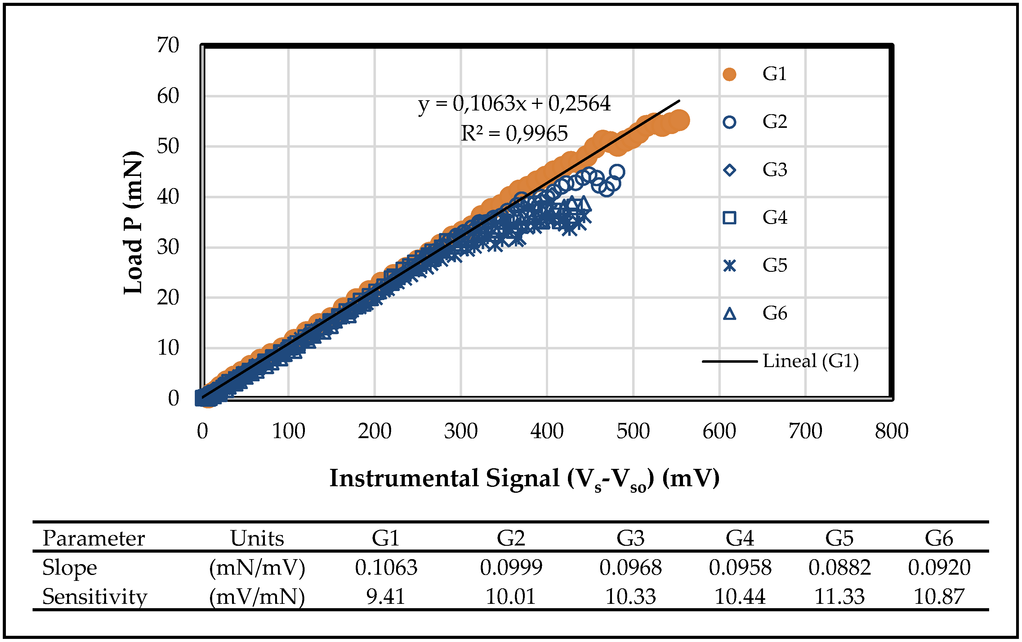
The device’s sensitivity is in the range of 9 to 18 mV/mN, depending on the location of the embedding region (near or within the sensitive area of the strain gauge as shown in Figure 1). Graphically, Figure 3 shows that the change in device output signal explains more than 99% of the load variability for strain gauges G1 to G6. Therefore, there is a high positive correlation between the load and the instrumental signal of the new device, where the variation in sensor sensitivity is attributable to manufacturing differences. There is high linearity within 30% to 80% of the maximum load because the sensors are, by design, within the elastic range.
In general, the sensor was tested for loads between 0 and 100 mN, showing high levels of linearity between load and instrumental signal and of lateral displacement between 0 and 1 mm, without generating gauge delamination or residual deformation effect and with an affordable cost and consumption. However, the experimental setup to measure shear stress in channels’ beds is expensive. The order of magnitude of detectable forces is less than 1 N/m2. On the other hand, the bed shear stress in open channels is in the order of 1–10 N/m2 [25,26,27,28]. In this case, the most relevant characteristic is that the dimension of the device is small enough to avoid significant interferences in the flow. It has to be noticed that there is room for improving: (1) the sensor embedding procedure to attain perfect embedding and (2) the capture of the device’s output signal.
Currently, it is difficult to provide an accurate estimation of the resolution and the minimum detectable force for the proposed device. However, an appropriate estimate is that the precision for the force is 2.5 mN and for the device’s output signal is 0.17 mV; therefore, the shear stress resolution would be 0.1 mN.
3. Results and Discussion
3.1. Load and Instrumental Signal Behavior in the Bending Tests
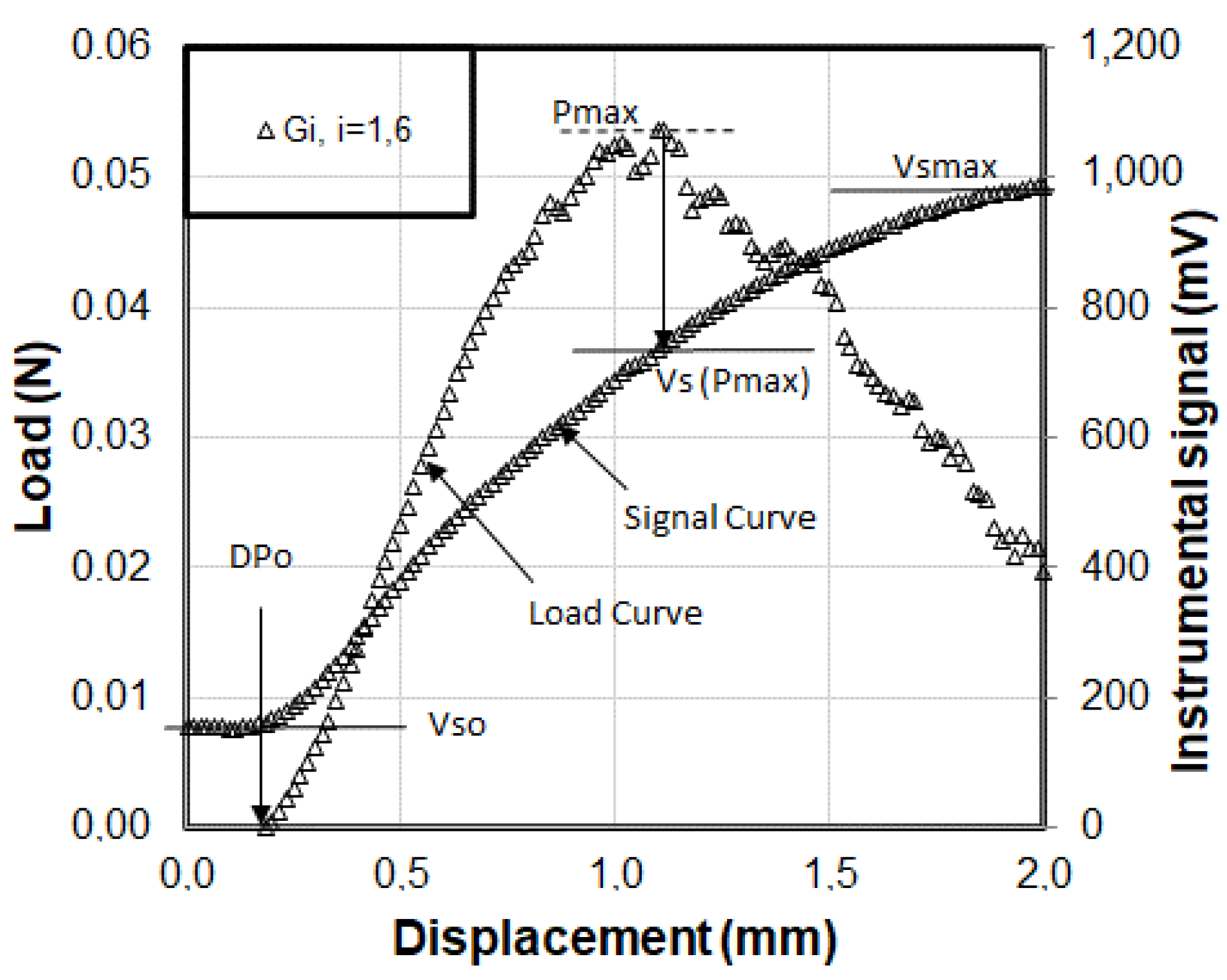
Figure 4 shows the typical development of the average curves of load and instrumental signal in the two-point bending tests relative to the displacement of the loading nose.
The average and the variation coefficients of the generic parameters for each sensor, such as the maximum instrumental signal (Vsmax), the instrumental signal at the beginning of the test (Vso), the instrumental signal at maximum load (Vs (Pmax)), the maximum load (Pmax), and the displacement when the loading nose touches the strain gauge (DPo) are determined and presented in Table 2.
Different mean DPo and Vso values were observed for each sensor and throughout the test repetitions, which can be attributed to experimental errors. These errors occurred due to difficulties in determining the moment when the surface of the strain gauge was touched by the loading nose and due to the initial settling of the measuring system of the strain gauge. Consequently, new uncertainties that have a significant impact on the behavior of the instrumental signal are posed in the estimation of Vso (see Table 3). Furthermore, the value for the maximum load (Pmax) was consistent for each strain gauge in all of the repetitions (see Table 2). However, the magnitude of Pmax differed significantly for each strain gauge, which is attributed to the position of the embedment and an inverse relationship between load and position of the loading nose [18]. Then, Pmax diminished as the embedment moved away from the central axis of the sensing area of the strain gauge. Hence, when the distance of xo increases, a lower total applied load is required to maintain the maximum bending moment constant in the area of embedment. Therefore, due to the dimensions of the tested material, new uncertainties concerning the measuring of xo are introduced.
In Table 2, the average values of the generic parameters are different for each sensor due to the characteristics of the tests presented in Table 1. This is attributed to the position of the embedment in the sensing area of the strain gauge and to the absence of a calibration process to adjust the display of the data acquisition system to zero.
The repeatability of the tests was determined due to the low value of the coefficients of variation (CV) observed for the instrumental signal (less than 1%) and the load (less than 7%), which validated the measuring systems. Thus, there is no influence of the measuring systems on the trends shown in the tests for each sensor, which implies that the variations or differences between them were only due to experimental errors.
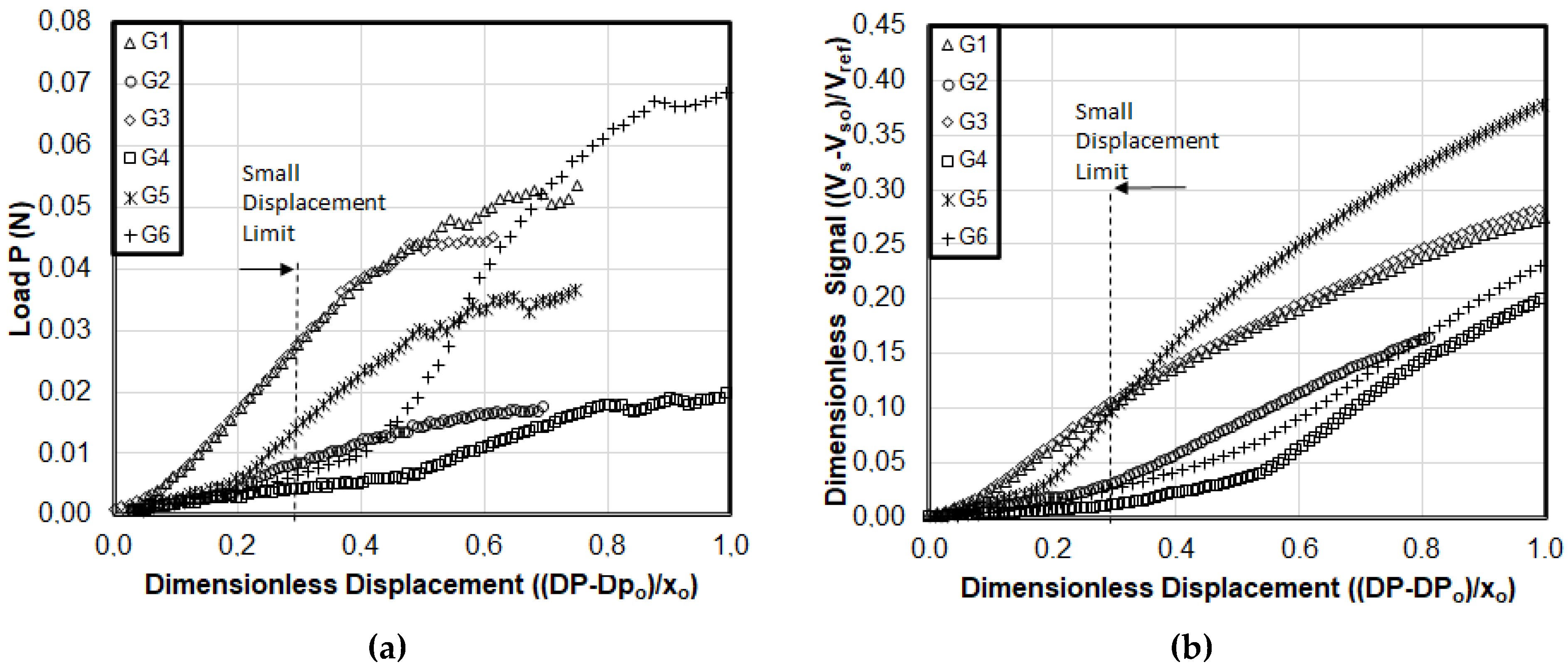
The average performance of the load and the instrumental signal for each sensor in the two-point bending tests is shown in Figure 5a,b, respectively. In Figure 5, the displacement value considered as small-displacement limit (SDL) is shown by a vertical dashed line [29].
In Figure 4 and Figure 5, it is observed that the sensors were subjected to large lateral displacements through the two-point bending tests. Similarities and differences between the average load–displacement and instrumental signal–displacement curves were found. A non-linear relationship between both the load and the instrumental signal and the lateral displacement was observed in all tests performed. The test repetitions showed a consistent trend for the load and the instrumental signal, namely, a third-order polynomial trend line for the whole range of the lateral displacement of the sensor. Furthermore, it is observed that the slope of the load–displacement curve changes sign when the lateral displacement of the sensor exceeds the maximum load value (Pmax). In contrast, the slope of the instrumental signal–displacement curve diminishes when the lateral displacement reaches its maximum value (Vsmax) (see Figure 5b and Table 2).
Within the SDL, a linear relationship can be observed in almost all of the responses of the average load–displacement and instrumental signal–displacement curves. This linear relationship can be extended beyond the SDL value up to lateral displacements induced by loads close to 80% of the maximum load, owing to the flexibility of the material used (strain gauges). This is consistent with the classical beam theory or the plate theory, as well as with the hypothesis proposed in this study. In addition, minimum slopes for the load–displacement and instrumental signal–displacement curves were observed for loads lower than 20% of the maximum load. This is attributed to the initial settling of the material when the surface of the sensing area was touched by the loading nose (G1, G3, and G5) or when the sensor was turned from its initial position owing to the absence of a perfect embedment (G4 and G6). Moreover, for lateral displacements larger than 0.5 times the xo value and that exceeded 80% of the maximum load, a loss of linearity was observed. This can be attributed to the loss of friction between the loading nose and the surface of the sensor. Additionally, the variation on the slopes of the curves can be attributed to the fact that the greater the lateral displacements to which the strain gauges were subjected, the lower the load required to maintain the maximum bending moment.
Finally, in Figure 5a,b, two types of behavior can be observed from the relationship between load–displacement and instrumental signal–displacement. This can be explained according to the position of the loading nose concerning the embedment of the strain gauge. The first type of behavior corresponded to an immediate response of the instrumental signal and the load on the sensor caused by the lateral displacement induced by the loading nose on those strain gauges embedded between 30% and 45% of the central axis of their sensing areas (sensors G1 and G3). The second type of behavior corresponded to a slow response of the instrumental signal and the load on the sensor when the embedment was located in the center or on the edge of the sensing area of the sensor (sensors G2, G4, and G6). Moreover, large lateral displacements were required to induce changes in the electrical resistance of the sensing area due to the absence of a perfect embedding of the strain gauge.
3.2. Relationship between Load and Instrumental Signal
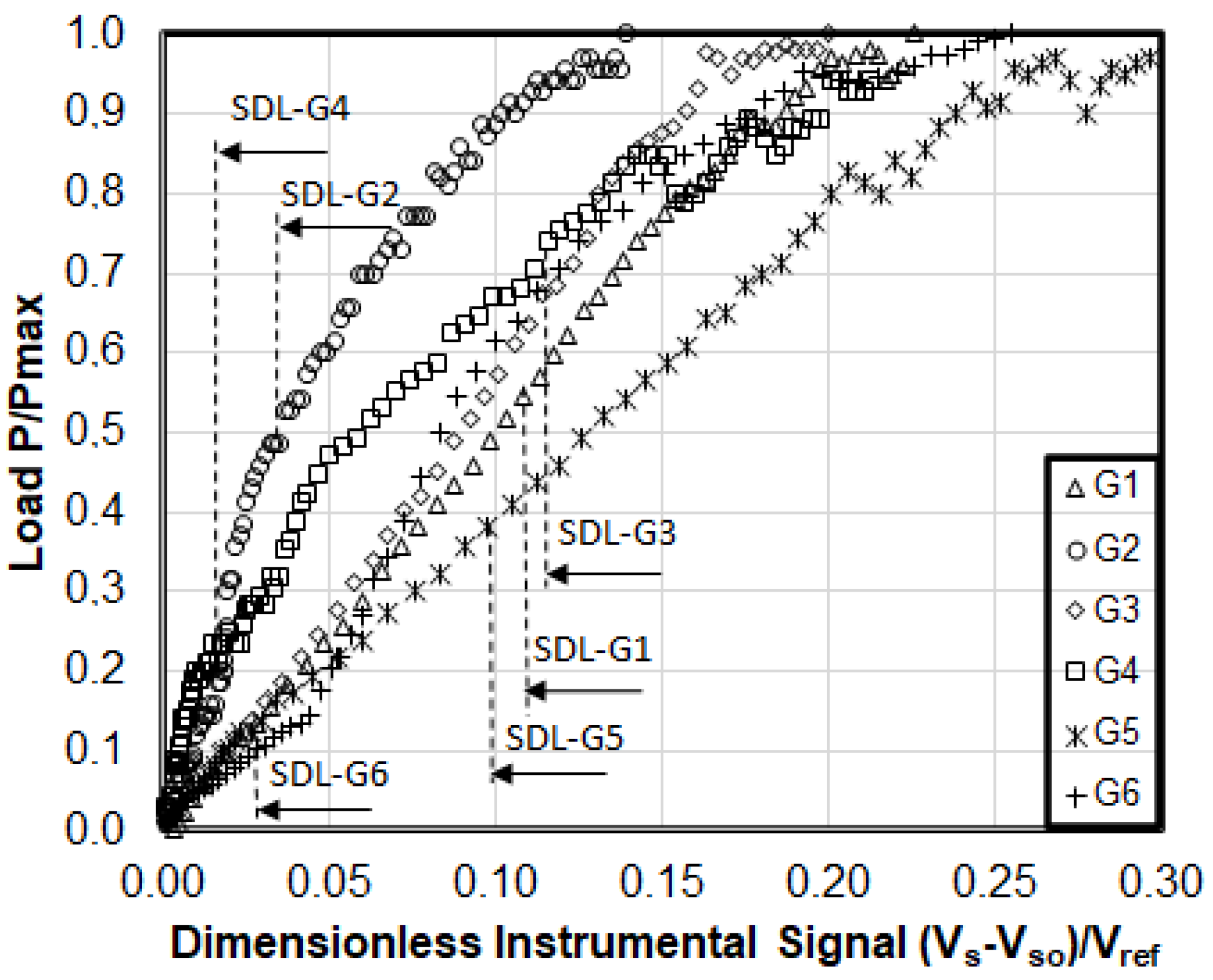
Figure 6 shows the dimensionless average load–instrumental signal curve obtained in the two-point bending tests for the dataset about load and instrumental signal lower than the maximum load (Pmax) at 1-s time intervals. Additionally, the figure shows that the SDL as a vertical dashed line, which corresponds to the ratio between the lateral displacement of the strain gauge and the position of application of the loading nose concerning the embedment, δB/xo, equals 0.3 [29].
For the loading range between 20 and 80 percent of maximum load, a linear model between the load (mN) and the instrumental signal (mV) was established. The parameters of the model, intercept (mN) and slope (mN/mV), are determined and presented in Table 3. The loading range was proposed to avoid the influence of the initial settling of the sensor, the effect of the loss of friction of the loading nose for large displacements, and the effect of the instrumental signal at the beginning of the test (Vso). In addition to this, in Table 3, the confidence interval and the probability of the F value of Fisher, obtained through the regression analysis, are presented for each parameter.
In Figure 6, a positive, dimensionless relationship between the load and the instrumental signal on each strain gauge is observed for the whole range of load values between zero and the maximum load [0, Pmax]. In the bending tests, two trends in the load–instrumental signal relationship were identified, which are explained by the position of the embedment relative to the strain gauge. These trends coincide with the results obtained in Figure 4.
The first trend was a significant linear relationship that showed a coefficient of determination greater than 0.99 for all loading ranges, including the lateral displacements greater than the SDL. It corresponded to the embedment ratios between 0.3 and 0.45 (G1, G3, and G5). For these trends, the estimation error did not exceed 5% of the measured value (see Figure 7).
The second trend corresponded to the strain gauges embedded on the edge or in the center of the sensing area (G2, G4, and G6) that showed a positive, non-linear relationship between load and instrumental signal. For small lateral displacements of the sensor, the linear trend between the load and the instrumental signal was significant. Nevertheless, the slope of the load–instrumental signal curve was two to four times greater than the slope of the first trend. This is due to the narrow range of variation of the instrumental signal compared to the range of variation of the load. This linear trend was significant for the whole loading range, but the coefficient of determination decreased to 0.93 (see Table 3) and the estimation errors exceeded 20% of the measured value (see Figure 7).
It is worthwhile to highlight that, in Figure 6, none of the sensors showed the initial settling of the measuring system in the bending tests illustrated in Figure 5. This can be attributed to the fact that the performance of the load sensor of the INSTRON is compared with the performance of the strain gauge itself, thereby annihilating the effects of the initial settling of the sensor and obtaining a linear relationship between the load and the instrumental signal from the beginning of the test. Thus, the loss of linearity of the load–instrumental signal curve for loads lower than 20% of the maximum load can be attributed to the absence of a perfect embedment of the sensor.
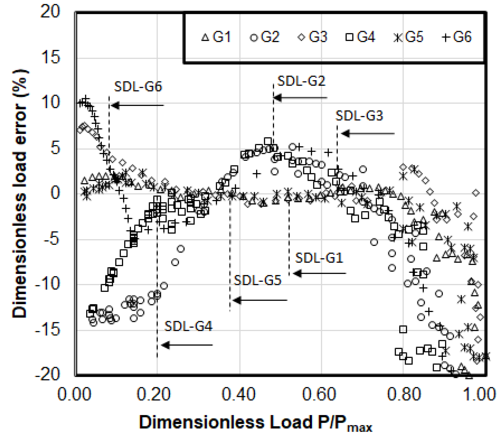
Additionally, for displacements greater than the SDL and close to 80% of the maximum load, an abrupt variation in the linear trend line, which has an error of overestimation greater than 15% of the measured value of the load, was observed (see Figure 7). This can be associated with the loss of friction between the loading nose and the surface of the strain gauge.
In Table 3, it is observed that all the regression coefficients (slopes) of the linear model rejected the null hypothesis. Furthermore, significant differences in the magnitude of the slope of the linear model were identified between sensors, which implies that the regression coefficient was individual for each one. The mean values for the slope of the linear model were lower for the sensors G1, G3, and G5, which had an embedment ratio of 0.30–0.45 from the axis of the sensing area of the strain gauge. The confidence intervals for these sensors were narrower than those of G2, G4, and G6. On the other hand, the intercept values for G2, G4, G5, and G6 were significantly different from zero. This is attributed to a shift in the initial voltage of the instrumental signal, which was different from the initial value of the instrumental signal at the beginning of the test only for sensor G1 (see Table 2 and Table 3). Although the difference between the values of the instrumental signal, Vso, was greater than 18% for sensors G2 and G4, it was not considered significant because of the broad confidence interval of the intercept due to the absence of a perfect embedment. Thus, the Vso value was an important source of uncertainty for the linear model that only influenced the intercept of the model. This is due to the settling of the sensor before taking the load and determining the moment when the loading nose touched the surface of the sensor. Nevertheless, the uncertainties regarding the coupling time between the load and the instrumental signal were reduced by using 1-s time-weighted average intervals.
On the other hand, Figure 7 shows the approximation error concerning the maximum load of the linear model between load and instrumental signal, according to the dimensionless load (P/Pmax). In Figure 7, it can be noticed that the greatest relative errors of approximation of the linear model were presented for the strain gauges embedded on the edge or in the center of the sensing area (G2, G4, and G6), which implied an error in the specification of the regression model used. On the other hand, for the embedment ratios close to 0.30–0.45 from the central axis of the sensing area (G1, G2, and G4), the linear model adequately approached the data obtained between the values 0.2 and 0.8 of the dimensionless load and showed a relative error inferior to 5%. This can lead to the conclusion that the location of the embedment relative to the strain gauge was the main factor affecting the regression model. Provided that this embedment was located within 30% to 45% of the sensing area, a linear response between the load and the instrumental signal was obtained.
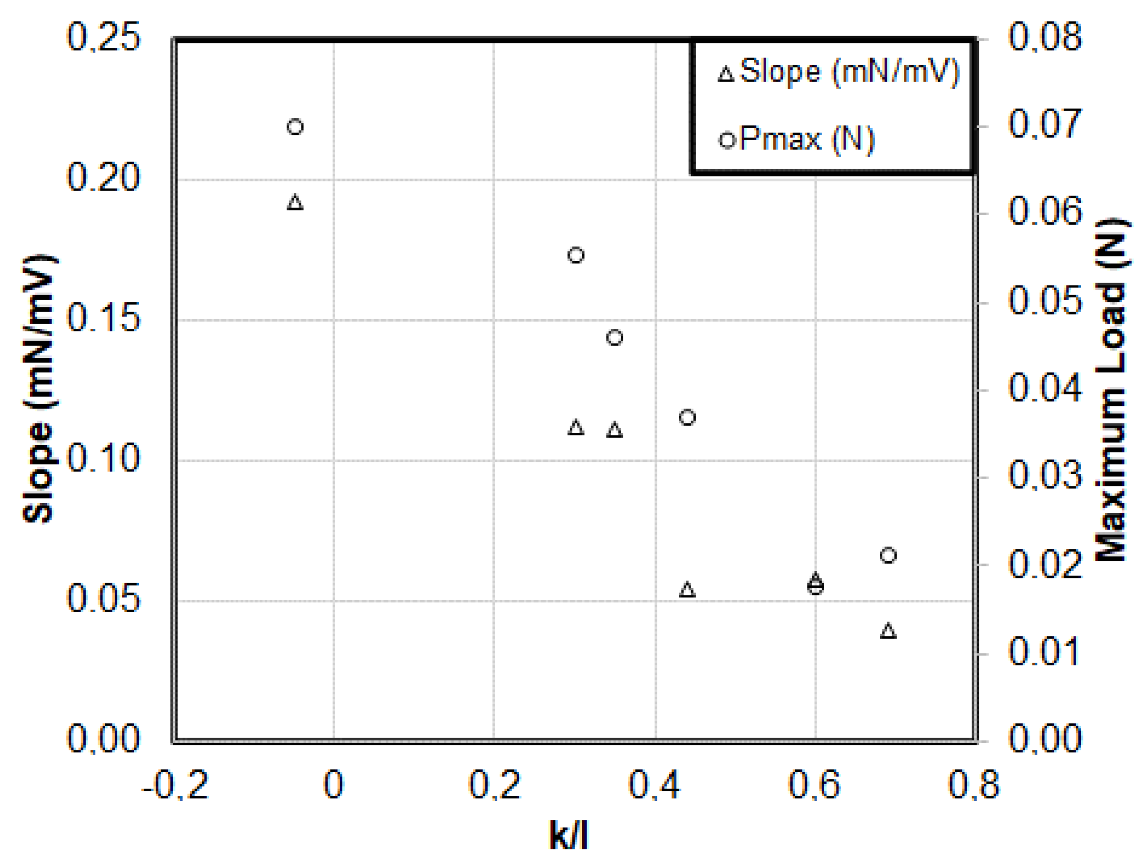
Alternatively, Figure 8 shows an inverse relationship between the slope of the load–instrumental signal curve and the location of the embedment concerning the central axis of the sensing area (embedment ratio). Figure 8 also shows an inverse relationship between the maximum load on each sensor and the embedment ratio. The foregoing is because both the maximum load and the slope of the load–instrumental signal curve were inversely related to the distance of application of the loading nose. This is because the location of the embedment (k) on the sensor was a fraction of the distance of application of the loading nose (xo). Thus, both Pmax and xo influenced the values of the parameters of the linear regression model, intercept, and slope; however, they did not affect the specification of the model, which depended solely on the location of the embedment within the sensing area.
In summary, the sensors G1, G3, and G5 showed better performances concerning the linear model between the load and the instrumental signal, for both great and small displacements of the strain gauge when the sensor was embedded between 30% and 45% of the axis of the sensing area, and approximation errors were inferior to 5%. The experimental load–displacement and instrumental signal–displacement curves (Figure 5a,b, respectively) showed a third-order polynomial trend for loads between zero and the maximum load. To obtain a linear relationship between the load and the instrumental signal, it is required that the load–displacement and instrumental signal–displacement curves be collinear; that is to say, the coefficients of the third-order polynomial model need to be perfectly scaled; and thus, both the load–displacement curve and the instrumental signal–displacement curve can measure the same phenomenon proportionally.
3.3. Measurements in an Experimental Open Channel
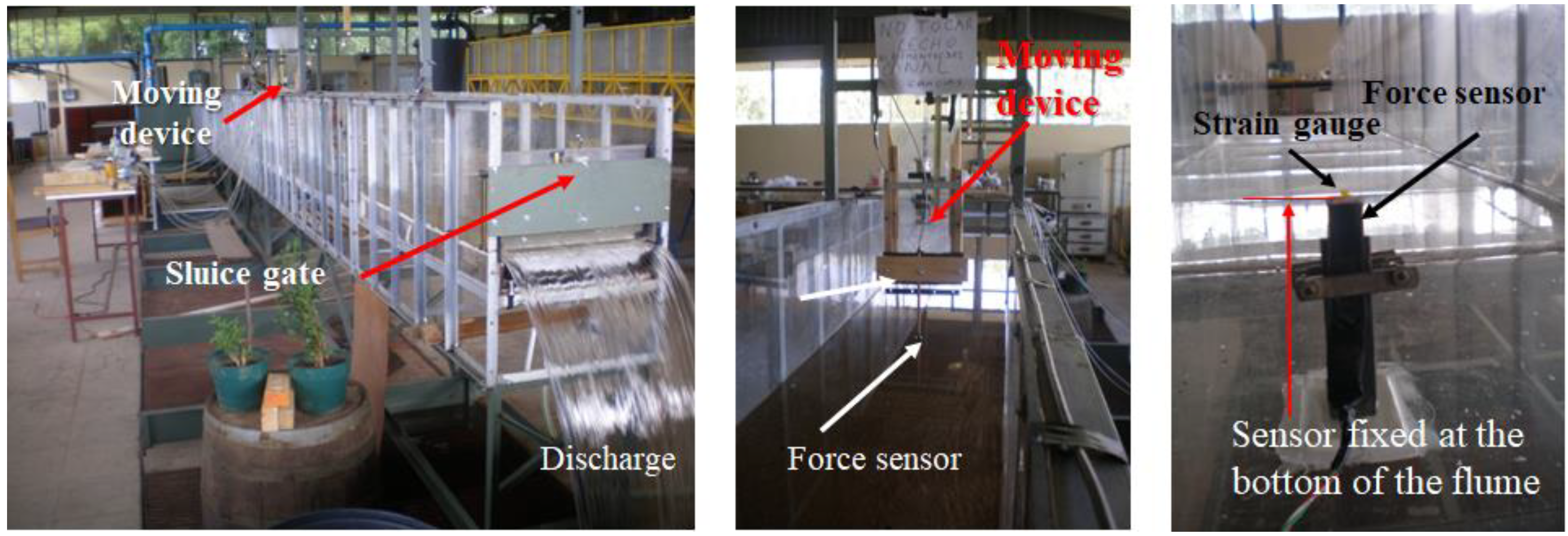
The proposed method shows a new setup to use a widely studied piezoresistive force micro-sensor based on a strain gauge as it derives the shear stress from bending (e.g., Pommois et al. [30], Allen et al. [31], Wang et al. [11], and Hua et al. [32]) instead of pure axial deformation. Preliminary results in controlled laboratory experiments were able to measure small forces due to local flow changes, as we observed a significant linear relationship between the change in strain gauge signal and the relative fluid-sensor velocity for flow depths greater than 5 cm, while flow depth less than 2 cm did not show changes in the strain gauges [33]. The experimental setup considered a granular bed and sensors located in the vicinity of the bed to relate flow depth to dynamic pressure inside the boundary layer and the pressure variation of the surface flow. The channel used was a rectangular prismatic section 0.48 m wide and 0.45 m high with an acrylic bed and walls. The laboratory flume is of variable slope, 12 m long, and was left with zero slope for experimental activities. The experimental test protocol proposed by Sepúlveda [33] was used, which adapted the ISO 3455:2007 standard for windlass calibration to the characteristics of operation and functioning of the sensor. Sepúlveda [33] assumed valid the principle of action and reaction of the force sensor on liquid water at rest, where it is expected that the constant movement of the sensor along the channel is equivalent to the movement of the fluid with the sensor at rest.
Changes in the coefficient of determination between flow velocity and the signal from the strain gauge were independent of temperature changes, but a high scattering of the data between tests is attributable to experimental errors such as orthogonality and/or twisting of the sensor in the direction of motion. In other experimental runs considering a moving fluid, the proposed sensor detected changes in flow depth, flow magnitude, and flow surface oscillations. Sensors located at the bed and near the bed (5.0 mm) showed a sudden decrease in the signal and then increased exponentially until the signal became constant. In contrast, for the sensor located 35 mm from the bed, the signal did not show a sudden decrease but an exponential and oscillatory increase consistent with the flow pressure gradient, until it reached a plateau. The magnitude of the instrumental signal change correlated positively with flow magnitude only for the sensor located 35 mm from the bed in all tests. Differences in response related to the location are due to the presence and influence of the boundary layer at the bed that affects the response of the signal. The sensor located outside the boundary layer (free zone) showed a coherent development with the changes of the flow variables. For sensors located inside the boundary layer, the hydraulic load was the most relevant variable measured by the instrumental signal. Figure 9 shows some pictures of the experimental test in an open channel with water in motion.
4. Conclusions
The linear model between the load and the instrumental signal was significant for all the sensors in the two-point bending tests, even for displacements above the SDL value. Moreover, the results were under the classical theory only for small displacements.
The sensors embedded within 30 to 45 percent of the axis of the sensing area showed a linear trend between the load and the instrumental signal, an approximation error of the load inferior to 5 percent, and a coefficient of determination greater than 0.99. The sensors embedded on the edge and in the center of the sensing area of the strain gauge presented a significant linear trend, an approximation error of the load greater than 15 percent, and a coefficient of determination between 0.93 and 0.98. This was due to the error of specification of the model for these cases.
For loads inferior to 20 percent of the maximum load, a loss of linearity was observed in the bending tests, which is attributed to an initial shift because of a lack of perfect embedment; whereas for loads superior to 20 percent of the maximum load, a loss of linearity was observed that can be attributed to the loss of friction between the loading nose and the surface of the sensor.
The parameters of the linear model, intercept, and slope were observed to be unique for each sensor. The value of the slope was inversely proportional to the location of the embedment on the sensor. In contrast, the intercept was directly affected by the value of the initial instrumental signal, Vso, and constituted a source of error. Therefore, it is advisable to consider the Vso value as a parameter of adjustment of the regression equation to reduce the uncertainties in the linear model.
Finally, the strain gauge itself, subjected to pure bending, can be employed to measure forces of small magnitude, in the order of mN, through a linear relationship between the load and the instrumental signal, provided that it is embedded within 30 to 45 percent of the sensing area. However, to the best of the authors’ knowledge, the present study is an isolated attempt to use strain gauges for the direct measurement of shear stress in open channels. Thus, it was not possible to compare the sensitivity results shown in the present research against other studies.
Future studies may consider a FEM study that may determine pressure sensors’ sensitivity in terms of device dimensions and linearity or improve the understanding of the dependence of various geometrical parameters on the overall sensor performance. In addition, for future research, a set of simulations to prove the capability of the proposed sensors may be conducted.
Author Contributions
Conceptualization, L.S. and D.R.; methodology, L.S. and D.R.; validation, L.S., D.R., and E.F.; formal analysis, L.S. and D.R.; investigation, L.S., D.R., and E.F.; resources, L.S.; data curation, L.S. and D.R.; writing—original draft preparation, L.S. and D.R.; writing—review and editing, E.F. and L.S.; visualization, L.S.; supervision, L.S. and D.R.; project administration, L.S.; funding acquisition, L.S. and E.F. All authors have read and agreed to the published version of the manuscript.
Funding
The APC was funded by the Universidad del Bío-Bío, Chile (Funding Number VRAPROYE-UBB2055).
Institutional Review Board Statement
Not applicable.
Informed Consent Statement
Not applicable.
Data Availability Statement
Not applicable.
Acknowledgments
The authors want to acknowledge the support provided by the Department of Agroindustry of the College of Agricultural Engineering at the Universidad de Concepción, Chile and by the Department of Civil and Environmental Engineering at the Universidad del Bío-Bío, Chile. In addition, the first author would like to acknowledge the scholarship provided by the National Commission for Scientific and Technological Research (CONICYT) to carry out his doctoral studies. Finally, Diego Rivera thanks the support from the Water Research Center for Agriculture and Mining, CRHIAM (ANID/FONDAP/15130015).
Conflicts of Interest
The authors declare no conflict of interest.
References
- Liang, Q.; Zhang, D.; Coppola, G.; Wang, Y.; Wei, S.; Ge, Y. Multi-Dimensional MEMS/Micro Sensor for Force and Moment Sensing: A Review. IEEE Sens. J. 2014, 14, 2643–2657. [Google Scholar] [CrossRef]
- Cheng, N.-S.; Nguyen, H.T. Hydraulic Radius for Evaluating Resistance Induced by Simulated Emergent Vegetation in Open-Channel Flows. J. Hydraul. Eng. 2011, 137, 995–1004. [Google Scholar] [CrossRef]
- D’Ippolito, A.; Calomino, F.; Alfonsi, G.; Lauria, A. Flow Resistance in Open Channel Due to Vegetation at Reach Scale: A Review. Water 2021, 13, 116. [Google Scholar] [CrossRef]
- Tinoco, R.O.; San Juan, J.E.; Mullarney, J.C. Simplification bias: Lessons from laboratory and field experiments on flow through aquatic vegetation. Earth Surf. Process. Landf. 2020, 45, 121–143. [Google Scholar] [CrossRef]
- Huai, W.; Li, S.; Katul, G.G.; Liu, M.; Yang, Z. Flow dynamics and sediment transport in vegetated rivers: A review. J. Hydrodyn. 2021, 33, 400–420. [Google Scholar] [CrossRef]
- Errico, A.; Lama, G.F.C.; Francalanci, S.; Chirico, G.B.; Solari, L.; Preti, F. Flow dynamics and turbulence patterns in a drainage channel colonized by common reed (Phragmites australis) under different scenarios of vegetation management. Ecol. Eng. 2019, 133, 39–52. [Google Scholar] [CrossRef]
- Duan, Y.; Zhong, Q.; Wang, G.; Zhang, P.; Li, D. Contributions of different scales of turbulent motions to the mean wall-shear stress in open channel flows at low-to-moderate Reynolds numbers. J. Fluid Mech. 2021, 918, A40. [Google Scholar] [CrossRef]
- Bashirzadeh, Y.; Qian, S.; Maruthamuthu, V. Non-intrusive measurement of wall shear stress in flow channels. Sens. Actuators A Phys. 2018, 271, 118–123. [Google Scholar] [CrossRef]
- Naughton, J.; Sheplak, M. Modern skin friction measurement techniques—Description, use, and what to do with the data. In Proceedings of the 21st Aerodynamic Measurement Technology and Ground Testing Conference, Denver, CO, USA, 19–22 June 2000; American Institute of Aeronautics and Astronautics: Reston, VI, USA, 2000; pp. 1–27. [Google Scholar]
- Örlü, R.; Vinuesa, R. Instantaneous wall-shear-stress measurements: Advances and application to near-wall extreme events. Meas. Sci. Technol. 2020, 31, 1–19. [Google Scholar] [CrossRef]
- Wang, J.; Pan, C.; Wang, J. Characteristics of fluctuating wall-shear stress in a turbulent boundary layer at low-to-moderate Reynolds number. Phys. Rev. Fluids 2020, 5, 074605. [Google Scholar] [CrossRef]
- Sheplak, M.; Cattafesta, L.; Nishida, T.; McGinley, C. MEMS Shear Stress Sensors: Promise and Progress. In Proceedings of the 24th AIAA Aerodynamic Measurement Technology and Ground Testing Conference, Portland, OR, USA, 28 June–1 July 2004; American Institute of Aeronautics and Astronautics: Reston, VI, USA, 2004; p. 13. [Google Scholar]
- Wei, J. Silicon MEMS for Detection of Liquid and Solid Fronts. Ph.D. Thesis, Delft University of Technology, Delft, The Netherlands, 2010. [Google Scholar]
- Haritonidis, J.H. The Measurement of Wall Shear Stress. In Advances in Fluid Mechanics Measurement; Springer: Berlin/Heidelberg, German, 1989; pp. 229–261. [Google Scholar]
- Kolitawong, C.; Giacomin, A.J.; Johnson, L.M. Invited Article: Local shear stress transduction. Rev. Sci. Instrum. 2010, 81, 1–20. [Google Scholar] [CrossRef] [PubMed]
- Patel, B.; Srinivas, A.R. Validation of experimental strain measurement technique and development of force transducer. Int. J. Sci. Eng. Res. 2012, 3, 1–4. [Google Scholar]
- ASTM D747-10; Standard Test Method for Apparent Bending Modulus of Plastics by Means of a Cantilever Beam. ASTM International: West Conshohocken, PA, USA, 2019.
- Timoshenko, S.; Gere, J.M. Mechanics of Materials; Van Nostrand Reinhold, Co.: New York, NY, USA, 1972. [Google Scholar]
- Ortiz Berrocal, L. Resistencia de Materiales, 3rd ed.; McGraw-Hill Interamericana de España S.L.: Madrid, Spain, 2007; ISBN 844-815-6331. [Google Scholar]
- Tian, B.; Zhong, Y.; Li, R. Analytic bending solutions of rectangular cantilever thin plates. Arch. Civ. Mech. Eng. 2011, 11, 1043–1052. [Google Scholar] [CrossRef]
- Hahn, R.; Rosentreter, E.E. ASAE Standards 1991: Standards, Engineering Practices and Data; American Society of Agricultural Engineers: St. Joseph, MI, USA, 1991; ISBN 092-9355-13X. [Google Scholar]
- Müller, I.; Machado, R.; Pereira, C.; Brusamarello, V. Load cells in force sensing analysis—Theory and a novel application. IEEE Instrum. Meas. Mag. 2010, 13, 15–19. [Google Scholar] [CrossRef] [Green Version]
- Palomo, F.; Vega-Leal, A.; Galván, E. Problemas Resueltos de Instrumentación Electrónica, 3rd ed.; Ingeniería–Universidad de Sevilla: Sevilla, Spain, 2013; ISBN 978-84-472-1061-9. [Google Scholar]
- Gujarati, D.; Porter, D.C. Basic Econometrics, 5th ed.; McGraw-Hill Education: New York, NY, USA, 2008; ISBN 007-3375-772. [Google Scholar]
- Knight, D.W.; Sterling, M. Boundary Shear in Circular Pipes Running Partially Full. J. Hydraul. Eng. 2000, 126, 263–275. [Google Scholar] [CrossRef]
- Lashkar-Ar, B.; Fathi-Mogh, M. Wall and Bed Shear Forces in Open Channels. Res. J. Phys. 2010, 4, 1–10. [Google Scholar] [CrossRef]
- Pan, J.; Shen, H.T.; Cheng, N.-S. Bed and wall shear stresses in smooth rectangular channels. J. Hydraul. Res. 2021, 59, 847–857. [Google Scholar] [CrossRef]
- Singh, P.K.; Banerjee, S.; Naik, B.; Kumar, A.; Khatua, K.K. Lateral distribution of depth average velocity & boundary shear stress in a gravel bed open channel flow. ISH J. Hydraul. Eng. 2021, 27, 23–37. [Google Scholar] [CrossRef]
- ISO 14125:1998. Fibre-Reinforced Plastic Composites: Determination of Flexural Properties; ISO: Geneva, Switzerland, 2013; p. 18.
- Pommois, R.; Furusawa, G.; Kosuge, T.; Yasunaga, S.; Hanawa, H.; Takahashi, H.; Kan, T.; Aoyama, H. Micro Water Flow Measurement Using a Temperature-Compensated MEMS Piezoresistive Cantilever. Micromachines 2020, 11, 647. [Google Scholar] [CrossRef]
- Allen, N.; Wood, D.; Rosamond, M.; Sims-Williams, D. Fabrication of an in-plane SU-8 cantilever with integrated strain gauge for wall shear stress measurements in fluid flows. Procedia Chem. 2009, 1, 923–926. [Google Scholar] [CrossRef] [Green Version]
- Hua, D.; Suzuki, H.; Mochizuki, S. Local wall shear stress measurements with a thin plate submerged in the sublayer in wall turbulent flows. Exp. Fluids 2017, 58, 124. [Google Scholar] [CrossRef]
- Sepúlveda, R. Calibración de Sensores de Fuerza Inmersos en Agua en Un Canal de Laboratorio; University of Bío-Bío: Concepción, Chile, 2013. [Google Scholar]
Figure 1.
Proposed two-point bending test: (a) INSTRON and experimental setup for implementing the bending test (loading nose width 1.0 ± 0.05 mm), (b) scheme of the bending test and data recording, (c) details of the strain gauge embedment.
Figure 1.
Proposed two-point bending test: (a) INSTRON and experimental setup for implementing the bending test (loading nose width 1.0 ± 0.05 mm), (b) scheme of the bending test and data recording, (c) details of the strain gauge embedment.

Figure 2.
Scheme of the instrumental signal measurement during bending tests.

Figure 3.
Relationship between instrumental signal and load P.

Figure 4.
Generic parameters of the average load and instrumental signal curves from the bending tests.
Figure 4.
Generic parameters of the average load and instrumental signal curves from the bending tests.

Figure 5.
Average load and instrumental signal curves obtained from the two-point bending tests: (a) dimensionless load–displacement curve, (b) dimensionless instrumental signal–displacement curve.
Figure 5.
Average load and instrumental signal curves obtained from the two-point bending tests: (a) dimensionless load–displacement curve, (b) dimensionless instrumental signal–displacement curve.

Figure 6.
Dimensionless average load–instrumental signal curve from the bending tests using 1-s time-weighted average values.
Figure 6.
Dimensionless average load–instrumental signal curve from the bending tests using 1-s time-weighted average values.

Figure 7.
Estimation error of the dimensionless load, P/Pmax.

Figure 8.
Slope and maximum load versus embedment ratio.

Figure 9.
Experimental test in an open channel.


Table 1.
Dimensions of the strain gauge sensors and characteristics of the bending tests.
| Sensor Dimensions | Trial Characteristics | |||||||||
|---|---|---|---|---|---|---|---|---|---|---|
| Sensor | b (mm) | e (mm) | Lo (mm) | Lo/e | xo (mm) | Rep | xo/e | xo/Lo | k (mm) | T (°C) |
| G1 | 2.54 | 0.060 | 2.27 | 37.8 | 1.22 | 5 | 20.3 | 0.54 | 0.30 | 27.9 ± 0.4 |
| G2 | 2.58 | 0.055 | 3.25 | 59.1 | 2.30 | 2 | 41.8 | 0.71 | 0.60 | 26.4 ± 1.0 |
| G3 | 2.54 | 0.050 | 2.30 | 46.0 | 1.35 | 2 | 27.0 | 0.59 | 0.35 | 26.4 ± 0.6 |
| G4 | 2.58 | 0.065 | 2.53 | 38.9 | 1.68 | 2 | 25.8 | 0.66 | 0.69 | 26.6 ± 0.4 |
| G5 | 2.54 | 0.065 | 2.46 | 37.8 | 1.51 | 2 | 23.2 | 0.61 | 0.44 | 26.5 ± 0.4 |
| G6 | 2.52 | 0.065 | 1.88 | 28.9 | 1.00 | 3 | 15.4 | 0.53 | −0.05 | 19.2 ± 2.6 |
| Average | 2.55 | 0.060 | 2.45 | |||||||
Table 2.
Experimental values of generic parameters for load and instrumental signal.
| Sensor | Vsmax (mV) | CV (%) | Vso (mV) | CV (%) | Vs(Pmax) (mV) | CV (%) | Pmax (N) | CV (%) | DPo (mm) | CV (%) |
|---|---|---|---|---|---|---|---|---|---|---|
| G1 | 984.7 | 0.7 | 154.4 | 8.4 | 707.0 | 3.3 | 0.056 | 4.7 | 0.203 | 17.9 |
| G2 | 703.5 | 0.3 | 284.2 | 0.2 | 670.4 | 6.0 | 0.018 | 2.0 | 0.216 | 32.5 |
| G3 | 1159.6 | 0.5 | 348.0 | 3.1 | 872.8 | 0.5 | 0.046 | 5.1 | 0.092 | 38.2 |
| G4 | 906.8 | 0.2 | 363.1 | 1.9 | 903.8 | 0.3 | 0.021 | 1.7 | 0.291 | 12.1 |
| G5 | 1317.9 | 0.3 | 239.1 | 22.9 | 1052.3 | 3.7 | 0.037 | 7.0 | 0.233 | 30.4 |
| G6 | 1746.4 | 0.0 | 876.5 | 7.5 | 1530.8 | 3.4 | 0.070 | 4.5 | 0.095 | 94.6 |
| Average | 1014.5 | 0.4 | 277.7 | 7.3 | 841.3 | 2.8 | 0.035 | 4.1 | 0.207 | 26.2 |
Table 3.
Statistical parameters of the linear model between load and instrumental signal (p < 0.8Pmax).
Table 3.
Statistical parameters of the linear model between load and instrumental signal (p < 0.8Pmax).
| Intercept (mN) | Slope (mN/mV) | Vsoe | Diff | ||||||||
|---|---|---|---|---|---|---|---|---|---|---|---|
| Sensor | Lower Limit | Value | Upper Limit | Prob-F | Lower Limit | Value | Upper Limit | Prob-F | R2 | (mV) | (%) |
| G1 | −19.57 | −18.98 | −18.40 | 0.0000 | 0.1110 | 0.1124 | 0.1138 | 0.0000 | 0.999 | 168.96 | 9.4 |
| G2 | −15.40 | −13.45 | −11.50 | 0.0000 | 0.0529 | 0.0578 | 0.0627 | 0.0000 | 0.935 | 232.78 | −18.1 |
| G3 | −42.91 | −41.19 | −39.48 | 0.0000 | 0.1083 | 0.1113 | 0.1143 | 0.0000 | 0.997 | 370.15 | 6.4 |
| G4 | −11.68 | −10.78 | −9.87 | 0.0000 | 0.0380 | 0.0397 | 0.0414 | 0.0000 | 0.977 | 271.46 | −25.2 |
| G5 | −13.46 | −12.65 | −11.84 | 0.0000 | 0.0533 | 0.0546 | 0.0559 | 0.0000 | 0.997 | 231.62 | −3.1 |
| G6 | −188.05 | −170.55 | −153.06 | 0.0000 | 0.1754 | 0.1917 | 0.2079 | 0.0000 | 0.975 | 889.82 | 1.5 |
Publisher’s Note: MDPI stays neutral with regard to jurisdictional claims in published maps and institutional affiliations. |
© 2022 by the authors. Licensee MDPI, Basel, Switzerland. This article is an open access article distributed under the terms and conditions of the Creative Commons Attribution (CC BY) license (https://creativecommons.org/licenses/by/4.0/).
Share and Cite
MDPI and ACS Style
Santana, L.; Rivera, D.; Forcael, E. Force Measurement with a Strain Gauge Subjected to Pure Bending in the Fluid–Wall Interaction of Open Water Channels. Appl. Sci. 2022, 12, 1744. https://0-doi-org.brum.beds.ac.uk/10.3390/app12031744
AMA Style
Santana L, Rivera D, Forcael E. Force Measurement with a Strain Gauge Subjected to Pure Bending in the Fluid–Wall Interaction of Open Water Channels. Applied Sciences. 2022; 12(3):1744. https://0-doi-org.brum.beds.ac.uk/10.3390/app12031744
Chicago/Turabian StyleSantana, Luis, Diego Rivera, and Eric Forcael. 2022. "Force Measurement with a Strain Gauge Subjected to Pure Bending in the Fluid–Wall Interaction of Open Water Channels" Applied Sciences 12, no. 3: 1744. https://0-doi-org.brum.beds.ac.uk/10.3390/app12031744
Note that from the first issue of 2016, this journal uses article numbers instead of page numbers. See further details here.