
Measurement of Large-Sized-Pipe Diameter Based on Stereo Vision


Faculty of Mechanical Engineering and Automation, Zhejiang Sci-Tech University, Hangzhou 310018, China
*
Author to whom correspondence should be addressed.
Appl. Sci. 2022, 12(10), 5277; https://0-doi-org.brum.beds.ac.uk/10.3390/app12105277
Submission received: 25 April 2022
/
Revised: 19 May 2022
/
Accepted: 20 May 2022
/
Published: 23 May 2022
(This article belongs to the Topic Advanced Systems Engineering: Theory and Applications)
Abstract
:To address the lack of fast and high-precision in situ measurement of large-sized pipes in current industrial applications, a pipe-diameter-measurement method based on stereo vision is designed in this paper. By using multiple sets of binocular cameras to perform 3D reconstruction and integration of multiple laser markers projected on measured cross sections of pipes, the pipe diameter can be estimated. In this method, a measurement algorithm is adopted to enable automatic matching of feature points through affine distance transformation, and an optimized point-cloud-registration algorithm with normal-vector constraints is used to ensure measurement robustness. To verify the feasibility of the method, an experimental system was built under laboratory conditions, and three types of pipes with outer diameters from 285 mm to 325 mm were measured. The experimental results show that the relative error is within ±0.570% and the maximum repeatability standard deviation is 0.551 mm. The experimental results basically meet industrial standards, and the proposed method therefore has good application prospects.
1. Introduction
Large-sized pipes are widely used in construction, chemical, oil and gas, aerospace, and other sectors [1,2,3]. With the improvement of productivity, both users and manufacturers have put forward higher requirements for the quality of pipe products. In situ detection of pipe parameters can provide feedback on production status for earlier production stages, thus helping manufacturers to reduce production costs and improve production qualification rates. The diameter and perimeter of pipes are important pipeline quality parameters and play a key role in ensuring progress and quality of pipeline construction. In the case of out-of-spec pipe diameter, a large residual stress generates during pipe welding, resulting in decline of the mechanical properties of welds and compromised safety of pipelines [4]. However, most production lines nowadays still use Pi tape measure for manual pipe measurement and lack an efficient on-site monitoring system. Therefore, in the production process of large-sized pipes, real-time precise measurement and control of their size parameters has become an urgent task. At present, non-contact measurement has become a hot topic in the research field of pipeline-dimension-parameter measurement due to reasons such as avoidance of damage to measured objects and convenient operation.
In the field of laser scanning and ranging, Mekid et al. [5] proposed an ingenious method to realize roundness measurement by analyzing the relationship between displacement and scattered-light intensity. However, it did not adequately address problems such as insufficient measurement range and complicated maintenance. Schöch et al. [6] proposed a 3D coordinate-measuring system composed of two main subsystems: a 2D laser-triangulation system capable of scanning a complete cross section of a part and a moving platform that moves the part in the measurement plane. For a larger measurement range with fewer sensors, some researchers tend to use a fixed laser rangefinder to measure roundness, straightness, or concentricity of rotating pipes [7,8,9,10] or a rotary laser rangefinder to measure fixed pipes [11,12].
Although a laser rangefinder has high precision, it is expensive and complicated in maintenance. Such shortcomings can be overcome with the most advanced vision technology. Scholars have proposed various solutions based on monocular vision for quickly measuring straightness or roundness of rotationally symmetrical workpieces. In these solutions, cameras are first used to acquire continuous images of a rotating workpiece. Next, image processing and modeling analysis are performed on the acquired images. Finally, a measurement is obtained [13,14]. Based on a 3D model constructed from boundary curves or beelines of forgings captured in two images, Zatočilová [15] and Zhou [16] presented a similar measurement system with two high-resolution single-lens reflex cameras to compute the straightness of rotationally symmetric forgings. However, due to the weak surface texture of pipes, it is often hard to achieve the desired feature point matching. Some scholars have therefore applied the structured-light technique to pipe measurement [17,18,19]. Based on the homographic relationship between a projector and a camera used for measurement, the specific images projected on the surface of an entire pipe can be converted into three-dimensional spatial information. To obtain a larger measurement range, researchers have devised new schemes, such as mounting the line-structured light with a CCD (charge coupled device) on a servo motor and allowing movement and measurement along the axis of the pipe [20,21], using an omni-directional laser and an omni-directional camera for measurement [22] and merging the pipe profile information obtained with multiple groups of structured lights [23,24,25]. There are also some schemes that combine laser markers with stereo vision. For example, Jia [26] used intersections of laser stripes as feature points and extracted laser stripes using stereo vision. By contrast, more researchers tend to reconstruct laser stripes in a direct way [27,28] and derive the outer diameters of pipes directly from the length of laser stripes, which has much room for improvement in measurement accuracy.
In this paper, a large-sized-pipe-diameter-measurement method is designed based on stereo vision. In this method, multiple sets of binocular cameras are used to perform 3D reconstruction and point-cloud registration on laser markers projected on the cross section of a pipe under test so as to achieve rapid on-site measurement of pipe diameter. The following research is completed in this paper: a feature-point-matching algorithm is designed with the aid of affine distance transformation to realize exact matching of feature points; singular value decomposition (SVD) is used to solve the rigid-body transformation; normal-vector constraints are then added; and the Gauss–Newton method is adopted to improve the robustness and accuracy of the measurement algorithm. An experimental system is built to verify the proposed method under laboratory conditions.
2. Materials and Methods
2.1. Principle of Measurement and Algorithm
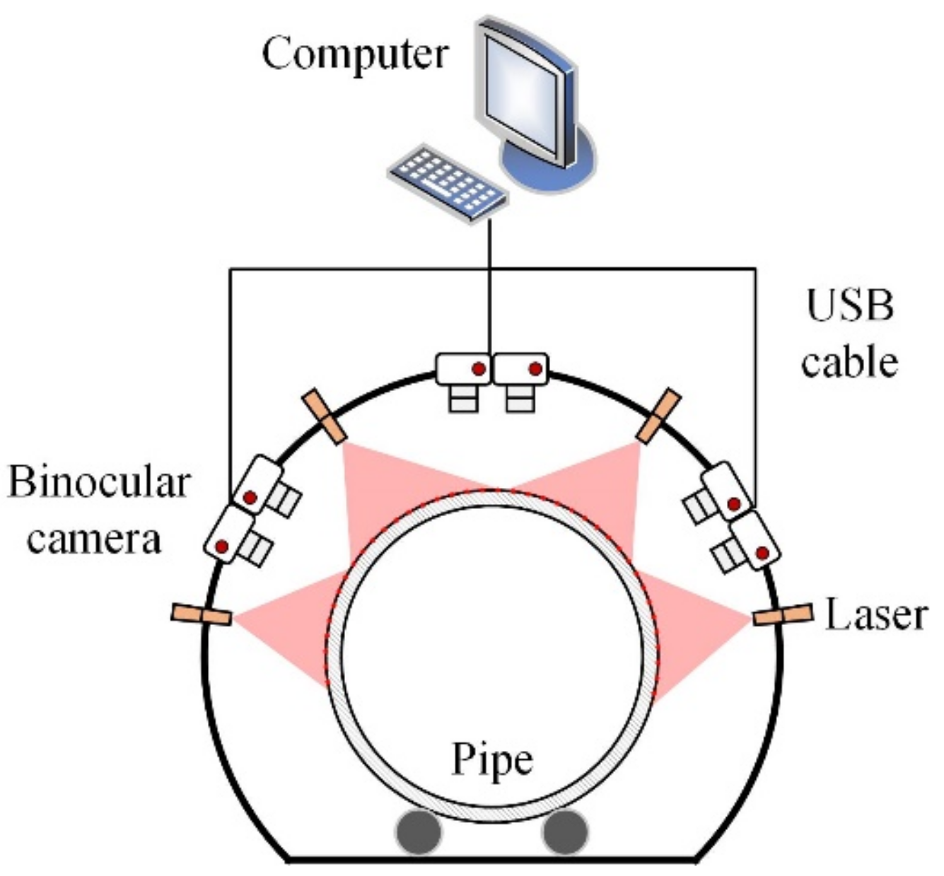
The schematic diagram of the proposed large-sized-pipe-diameter-parameter-measurement system is shown in Figure 1, which includes a digital image acquisition unit composed of three sets of binocular cameras, a marker projection unit composed of multiple lasers, a computer responsible for data processing, and a bracket for equipment installation.
The bracket spans the pipe under test and is kept as perpendicular to the central axis of the pipe as possible. Multiple lasers fixed on the bracket project a circle of laser markers on the surface of the pipe from different angles as the feature points of the cross section. At the same time, multiple sets of binocular cameras capture images of the pipe from different positions and communicate with the computer in real time through USB cables. After the feature points are extracted, a specific matching algorithm is used to achieve feature point matching and 3D reconstruction, and multiple sets of point clouds are obtained. Next, based on the implicit relationship between each group of point clouds, the corresponding matching points are matched and the rigid-body transformation is calculated to realize point-cloud registration. Finally, the spatial-circle-fitting algorithm is used for the registered point clouds to estimate the diameter of the measured pipe cross section.
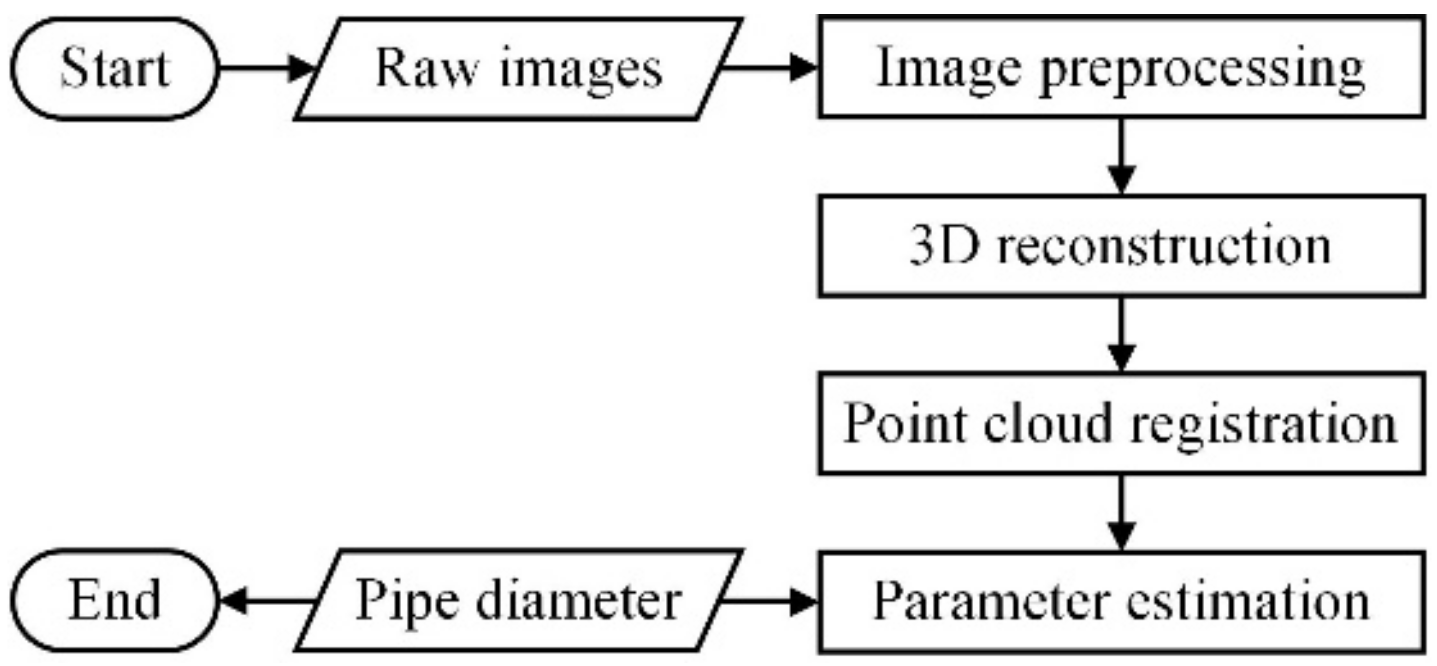
The measurement algorithm flow is shown in Figure 2. Raw images captured by multiple sets of binocular cameras are used as input. After image preprocessing, 3D reconstruction, point-cloud registration, and parameter estimation, the pipe diameter is finally obtained as output.
Image preprocessing includes steps such as camera calibration, image denoising and stereo correction. Its main function is to convert the raw images into clear images aligned horizontally with affine lines, which is the basis of the entire measurement algorithm.
In our study, feature points are extracted by identifying the center of the blob feature in the images with DoG (difference of Gaussian), and the corresponding algorithm flow is not further explained here. On the basis of image preprocessing, parameters, such as Gaussian standard deviation range, elliptical interval, and judgment threshold, can be set according to a priori knowledge so as to accurately and efficiently extract laser marks as feature points.
2.2. Three-Dimensional Reconstruction
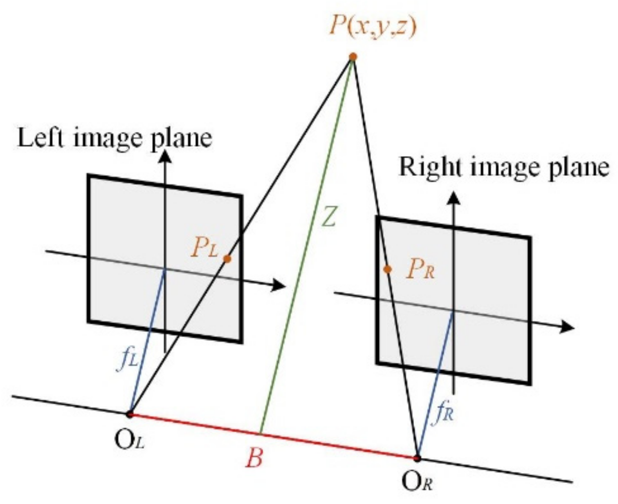
The principle of binocular vision is similar to that of human eye imaging. It analyzes the imaging difference of the same object in the three-dimensional space in the left and right cameras of a camera set and reconstructs the three-dimensional geometric information of the object based on the principle of triangulation.
Figure 3 shows the process of 3D reconstruction of images captured with the binocular camera based on the principle of triangulation ranging. Ol and Or are the optical centers of the left and right cameras, respectively, f is the focal length of the cameras, and B is the center distance between the two cameras. For a point P(x, y, z) in space, its projection points on the imaging plane of the left camera and that of the right camera are Pl(xl, yl) and Pr(xr, yr), respectively. From the similar relationship of the triangles, the distance Z between the measured point P and the camera baseline can be obtained as
In the left-camera coordinate system, three-dimensional restoration of the measured point P is performed, and its coordinates (xc, yc, zc) are expressed as
For any point on the image plane of the left camera, as long as a matching point can be identified on the image plane of the right camera, the three-dimensional coordinates of the point are derivable through point-to-point operations. In the course of feature point matching, a matching relationship is identified between a pair of images.
In the measurement method proposed in this paper, the markers projected on the surface of a pipe under test are regarded as feature points for extraction and matching purpose. The low density of feature points naturally leads to low efficiency in traditional feature point extraction and matching algorithms. Therefore, a special feature point extraction and matching algorithm is designed in this paper to realize feature point extraction by screening blob features with DoG and to match feature points based on affine distance transformation.
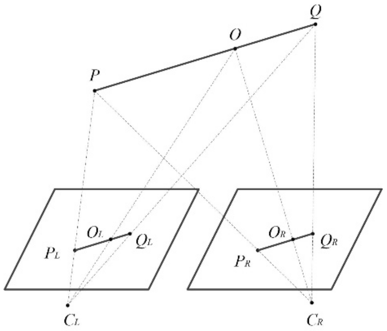
As shown in Figure 4, POQ is a straight line segment in space, and its projected line segments in the left and right cameras CL and CR are PLOLQL and PRORQR, respectively. According to the properties of affine transformation, the position order of points on the same line and the length proportion remain unchanged, namely
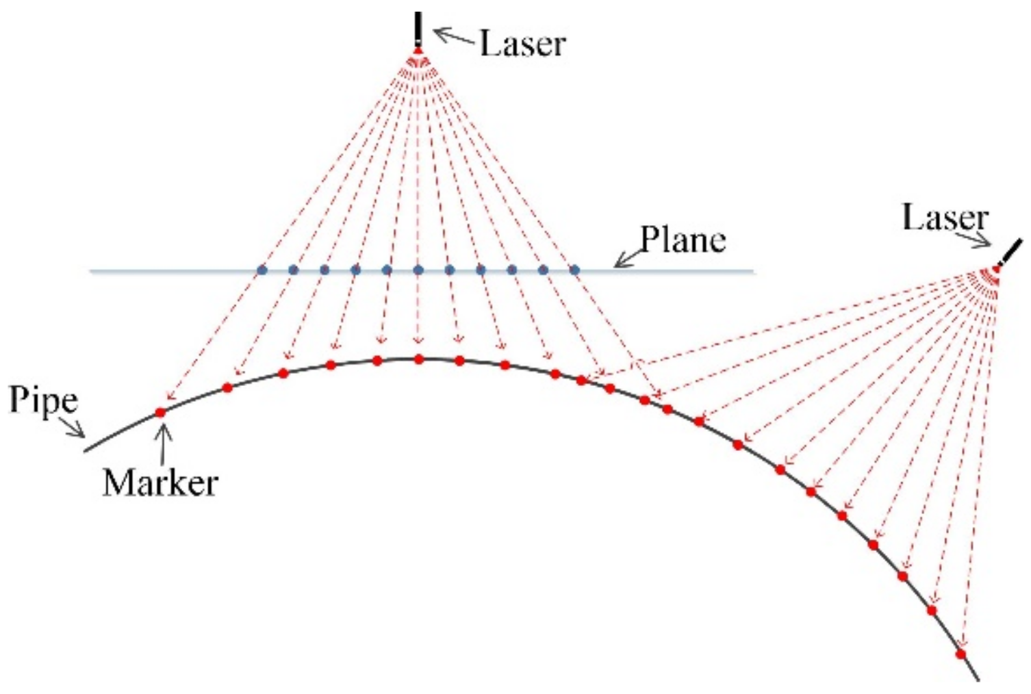
Figure 5 shows the distribution of laser markers on the pipe surface. A row of equidistant laser markers projects on the surface by the laser when the light-beam axis is perpendicular to the plane. However, when the laser is cast onto the surface of a pipe with large curvature, the distribution of laser markers is affected by the curvature. As a result, laser markers with different spacing form on the surface of the pipe. At the same time, the markers projected by multiple lasers also have overlapping areas, forming non-equidistant marker features on the surface of the pipe. On the other hand, due to the large curvature of the measured pipe and the small interval between the laser markers, the line segment formed by three adjacent laser markers can be approximately regarded as a straight-line segment, which satisfies the above-mentioned conditions of affine distance transformation.
In summary, when laser markers are used as feature points, the inconsistent spacing and affine-transformation properties of laser markers provide a basis for the matching of feature points. Taking an image captured by the left camera as an example, for three adjacent laser markers PLOLQL along the one-dimensional laser marker direction, their matching element is defined as the ratio of the PLOL pixel length to the PLQL pixel length, namely
FL and FR are the matching element sets of the images captured by the left and right cameras, respectively. To obtain the longest segment of the matching sequence in FL and FR, this paper uses dynamic programming for matching, whose corresponding state-transition equation is
where dp is the state-variable matrix; dp[i][j] is the current state, which represents the longest matching length of the first i matching elements of FL and the first j matching elements of FR; and dp[i − 1][j − 1] is the previous state. Then the optimal matching solution can be indicated by the position and length corresponding to the maximum element in the dp matrix.
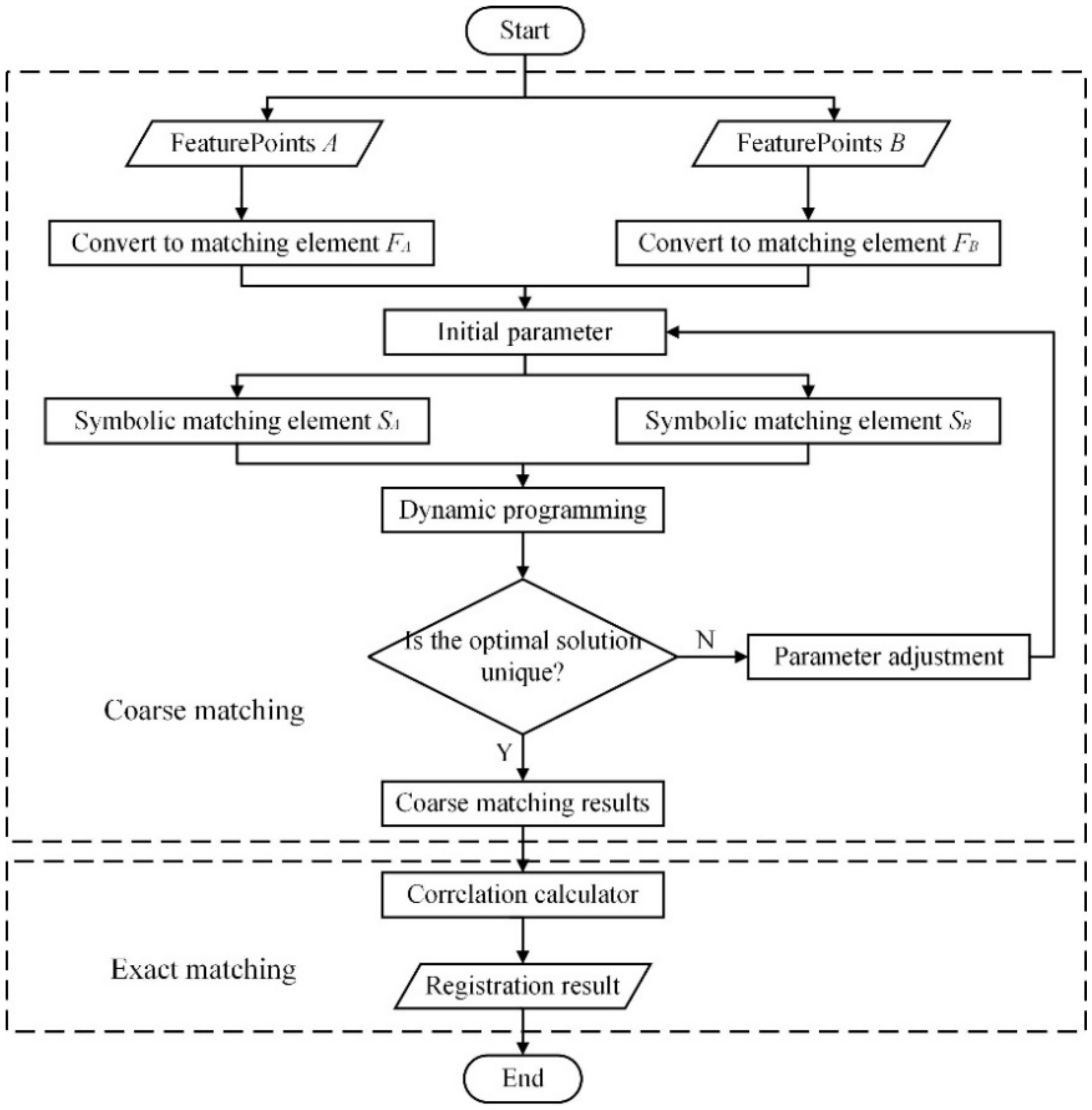
The flowchart of feature point matching is shown in Figure 6, which is divided into two steps: coarse matching and exact matching.
The specific coarse matching steps are as follows: (1) According to Formula (4), the feature points A and B extracted from the images captured by left and right cameras are converted into matching elements PA and PB, respectively; (2) Both matching elements PA and PB receive regular normalization to realize normal distribution. The slope between two adjacent points is then calculated. Based on the initial parameter n, the complete slope space is evenly divided into n regions, which are [0, 1, …n − 1]; (3) The matching elements are symbolized for regions corresponding to each slope in the slope sequence. The slopes are roughly classified by replacing every slope with the label of the region where the slope is located; (4) Dynamic programming is performed on the two groups of matching elements after symbolization. If the maximum element in the dp matrix occurs more than once, which means the optimal solution is not unique, the parameter n is adjusted and the process returns to the second step. Such iteration continues until a unique optimal solution is achieved; (5) In order to ensure the accuracy of matching, when the conditions for ending the iteration are met, the matching sequence numbers corresponding to the optimal solution and the sub-optimal solution are selected as the coarse matching results. It is noteworthy that the sub-optimal solution is the matching sequence corresponding to the second-largest element in the dp matrix.
During exact matching, correlation calculation is performed on the candidate matching results from coarse matching, and the result from the group with the highest degree of correlation is taken as the final matching result.
2.3. Point-Cloud Registration
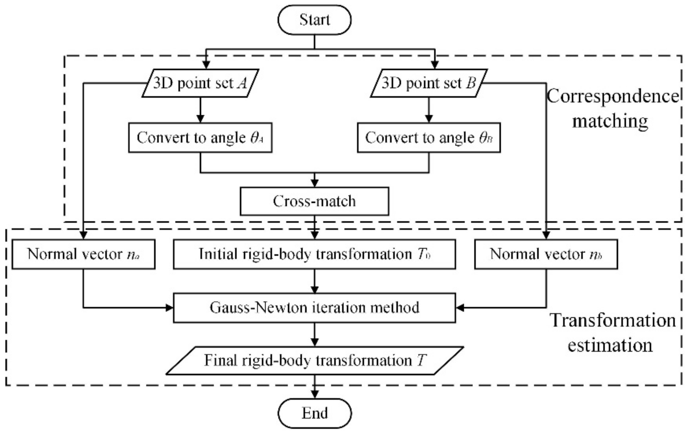
Each set of binocular cameras eventually provides a group of point clouds about a certain arc of the measured cross section, but, at this point, each group of point clouds has its own coordinate system and the different groups need to be registered for standardization in a single coordinate system. The flow chart of point-cloud registration is shown in Figure 7, which is divided into two parts: correspondence matching and transformation estimation.
In practical-application scenarios, the approximate relationship between the two cameras in each set is known: the right half of the feature points acquired by the left camera and the left half of the feature points acquired by the right camera are corresponding points. Therefore, in the correspondence-matching process, based on fitting of the circle center of each group of point clouds, the angle formed by two adjacent points and the center of the fitted circle is calculated. The two sets of angles are then moved toward each other continuously to enable calculation of angle correlation. The matching result with the highest degree of correlation is taken as the final matching result of corresponding points.
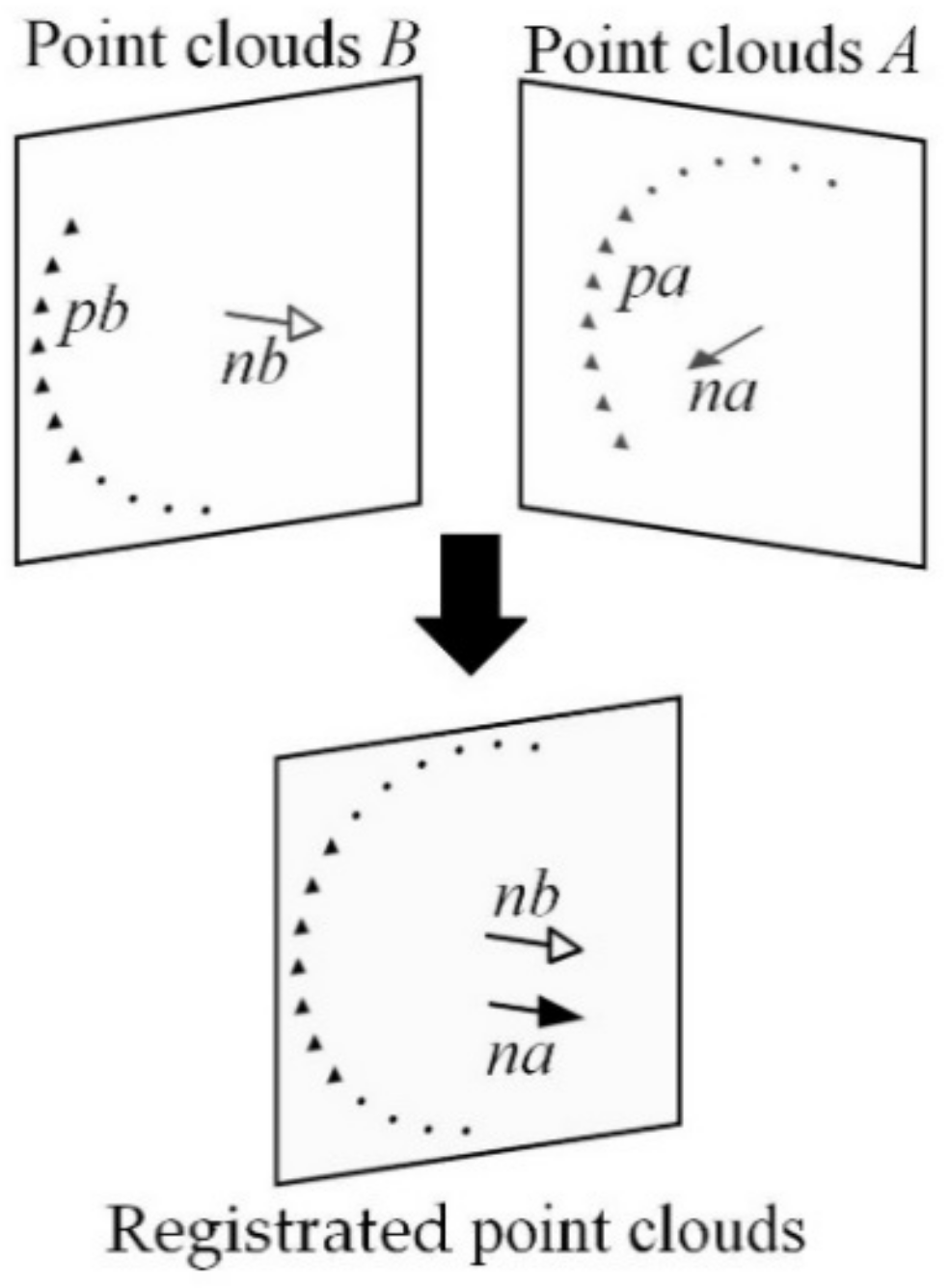
SVD is a widely used method for solving rigid-body transformations. It not only uses principal component analysis (PCA) to construct distance errors between point clouds but also solves rotation matrices and translation vectors with the least-squares method. However, due to factors such as ambient light and feature-point-extraction accuracy, there is noise in the reconstructed 3D point clouds. That is to say, the 3D points are not strictly on a plane. In the point-cloud registration of the section circle, the ideal transformation results of the two groups of point clouds is in the same plane and form an arc. However, since the traditional SVD only considers the Euclidean distance between corresponding points, it is easy to fall into a local minimum, resulting in an angular difference between the two groups of point clouds after conversion, which affects the measurement accuracy. Therefore, in this paper, the result of rigid-body transformation obtained by SVD is used as the initial value and the difference between the plane normal vectors of the two groups of point clouds is used as the constraint condition to construct a Newton–Gaussian solving algorithm. The schematic diagram of the algorithm is shown in Figure 8.
Points pa and pb are corresponding points of point clouds A and B, respectively, and na and nb are the normal vectors of the entire point clouds A and B. The matching vector is expanded to P = [pT nT]T. On the basis of the error function ei(T), an objective function T* is constructed:
where and , which is the information matrix. The weight of the normal-vector constraint is determined by changing λ.
With the Gauss–Newton iteration method, the objective function is minimized through local parameterization using incremental perturbations and the optimal T is solved through iterations. The incremental equation is expressed as
where is the approximate Hessian matrix and is the Jacobian matrix of error with respect to disturbance; , including the translation vector Δt and the imaginary part Δq of the four-element rotation unit; and .
The transformation-solving steps are described as follows: SVD is used to obtain the initial transformation T0. An objective function T* is constructed based on the normal vectors of two sets of correspondence points. For the k-th iteration, the increment ΔTk is calculated. If ΔTk is small enough, the iteration process is ended and the final rigid-body transformation T is taken as the output. Otherwise, the iteration process is repeated from the third step with Tk+1 = Tk + ΔTk.
2.4. Parameter Estimation
Through 3D reconstruction of feature points and point-cloud registration, 3D point clouds of the measured pipe cross section are obtained. However, it is also necessary to fit a three-dimensional circle to obtain the geometric center and diameter of the measured cross section and other dimensional information.
The least-squares method is a method for parameter estimation of regression models from the perspective of error fitting. It finds the best function matching of data by minimizing the squared sum of errors. Hence, we use the least-squares method for spacial circle fitting. We do not explain here the mathematical solution model of spacial circle fitting with least squares. Instead, we focus on how to establish an overdetermined equation based on plane fitting with the knowledge that the perpendicular bisector of the segment connecting any two points of a planar circle always passes the center of the circle.
For the three-dimensional point set X{[x1,y1,z1], [x2,y2,z2]…… [xn,yn,zn]}, the overdetermined equation can be established with least squares, and its planar normal vector N is obtained:
Since the perpendicular bisector of the segment connecting any two points of a planar circle always passes the center of the circle, the overdetermined equation is constructed again, and the coordinates C[x0,y0,z0] of the center of the circle are obtained:
where and .
Finally, twice the average distance from all points to the center of the circle is used as the diameter d of the fitted circle:
It is noted that the measurement method proposed in this paper uses only the upper profile of the pipe to evaluate the diameter. In precision coordinate measurement, the differences in the arc length of the sampling points and the ovality of the measured pipe lead to different deviations when evaluating the diameter by the least-squares method. Simulations and analysis are therefore carried out to investigate their relationships and to verify the rationality of the system design.
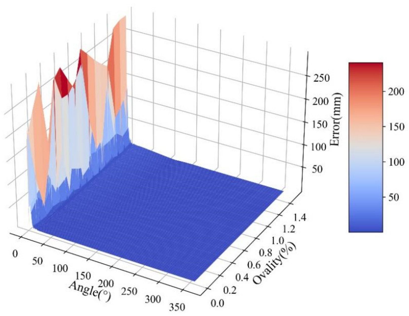
In simulations, the major axis of the ellipse is set to 300 mm and the ovality is set to vary from 0.0% to 1.5% with a step of 0.1%. The range of central angle corresponding to arc that envelopes the sampling points is set from 1° to 360° with a step of 1°, and each degree of central angle contains three the sampling points. Using the proposed method to calculate the diameter of simulated pipe, the error distribution of the pipe diameter is shown in Figure 9.
If the permitted error of the pipe diameter is within 1 mm, it is seen from the simulations that the maximum required central angle is 168°, considering the ovality varies from 0.0% to 1.5%. That is to say, to ensure the measurement accuracy of the diameter, the central angle enveloping the sampling points must be larger than 168°.
2.5. Experimental System
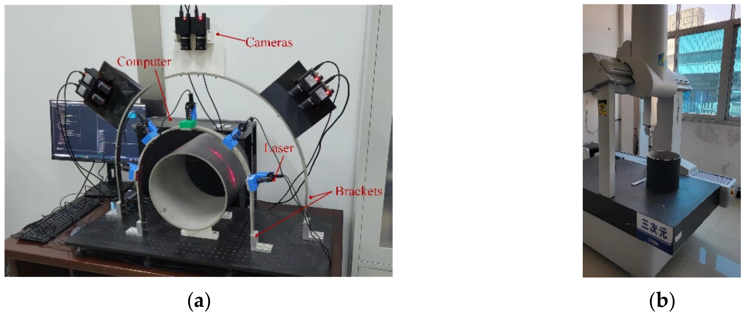
To verify the feasibility of the proposed method, an experimental system, as shown in Figure 10a, was built, which mainly consisted of an imaging module that included three sets of binocular cameras, a marker projection module composed of five lasers, a data processing module of a high-performance computer, and a bracket for equipment installation. Model QJY0816 industrial cameras with an image size of 2/3 inch were used in the experimental system, each equipped with an 8 mm fixed-focus lens and the field angle of 56.5 × 43.9°. According to the conclusion of the above simulations, it is a prerequisite for achieving high accuracy in diameter measurements to keep the central angle larger than 168°. Therefore, considering the field angle of typical industrial cameras and final-cost control in our study, three sets of binocular cameras were selected to form the experimental system, and the central angle corresponding to the measurement point was set at about 180°. The main computer components responsible for processing digital images were the Intel Xeon Gold 5218 and RTX3090.
In addition, to obtain high-precision measurement results as reference, we used the Hexagon brand Inspector Performance series Coordinate Measuring Machine (CMM) to measure the pipe. Figure 10b shows the site where the CMM was used to measure the diameter of the pipe. The accuracy of this type of CMM reaches 0.001 mm.
3. Results and Discussion
3.1. Effect of Feature-Point-Matching Algorithm
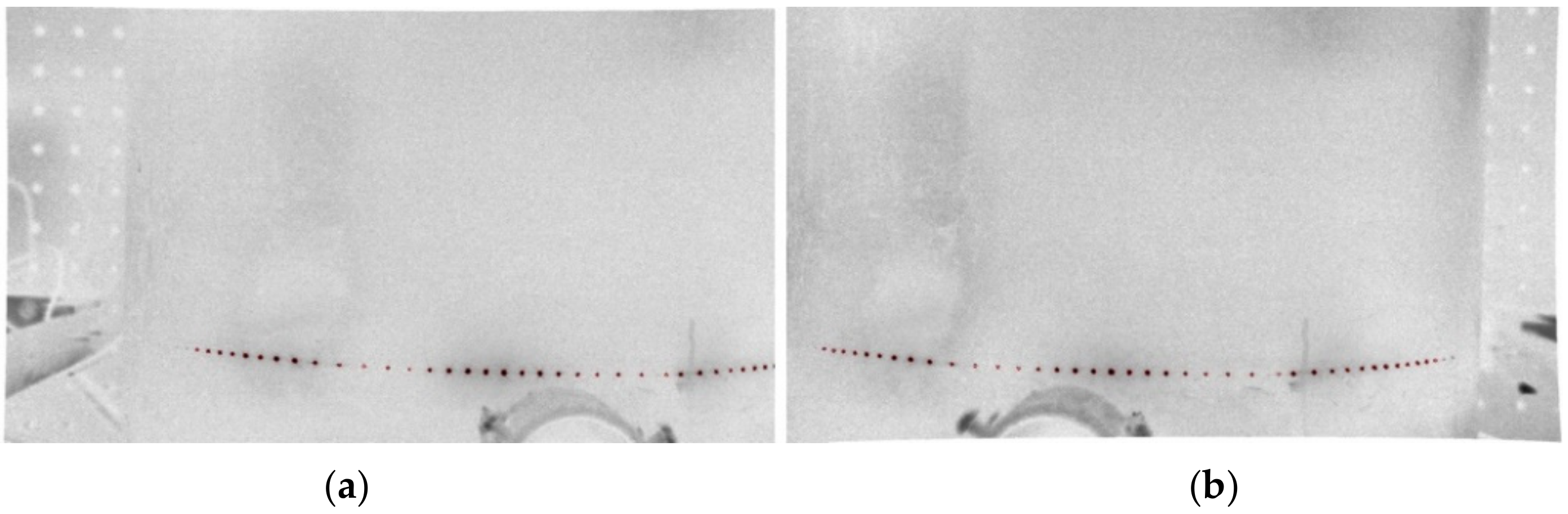
In this method, the markers projected by the lasers are used as the feature points, and the center of the markers is extracted by identifying the blob features with DoG. A section in the middle of the pipe with an outer diameter of 299 mm is selected for tests, and the actual feature-point-extraction results are shown in Figure 11, in which (a) and (b) show the feature-point-extraction results of the left camera and the right camera, respectively. It is seen from the figures that the markers projected on the surface of the pipe are almost completely identified and extracted, meaning that the expected effect is achieved.
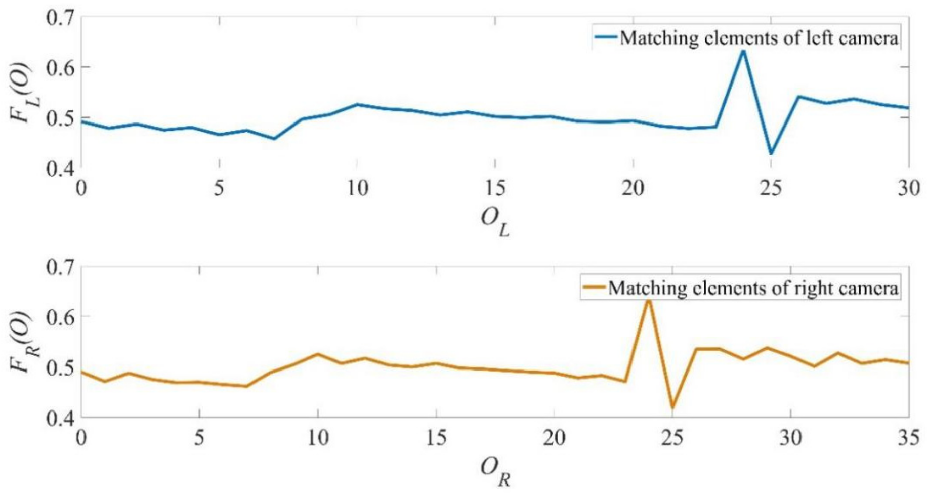
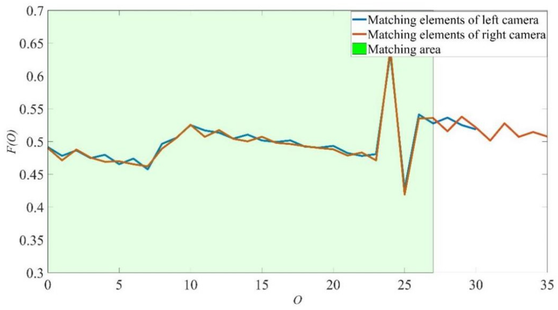
With the proposed feature-point-matching algorithm based on affine distance transformation, after the feature points are accurately extracted, the feature points provided by the left and right cameras are converted into matching elements FL and FR, respectively, according to Formula (4), as shown in Figure 12. It is not difficult to find that after the affine distance transformation, the markers experience obvious amplitude changes and no longer follow the original single and identical distributions. In particular, amplitude oscillation appears near the 24th matching element. These obvious features provide the basis for the correspondence matching.
The final matching effect is shown in Figure 13. The dark area displays the final matching result. It is found that despite the noise in the matching elements, the algorithm proposed in this paper still achieves correct matching of feature points satisfactorily. Many experiments have also proven that the accurate matching rate of this method can reach more than 98%.
3.2. Effect of Point-Cloud-Registration Algorithm
For most of the system running time, simply using SVD to solve for correspondence points in the point clouds can achieve the desired effect. However, due to factors such as noise or the small number of corresponding points, the transformation solution sometimes falls into a local minimum and the two groups of point clouds after rigid-body transformation have obvious angle differences, suggesting poor stability of the algorithm.
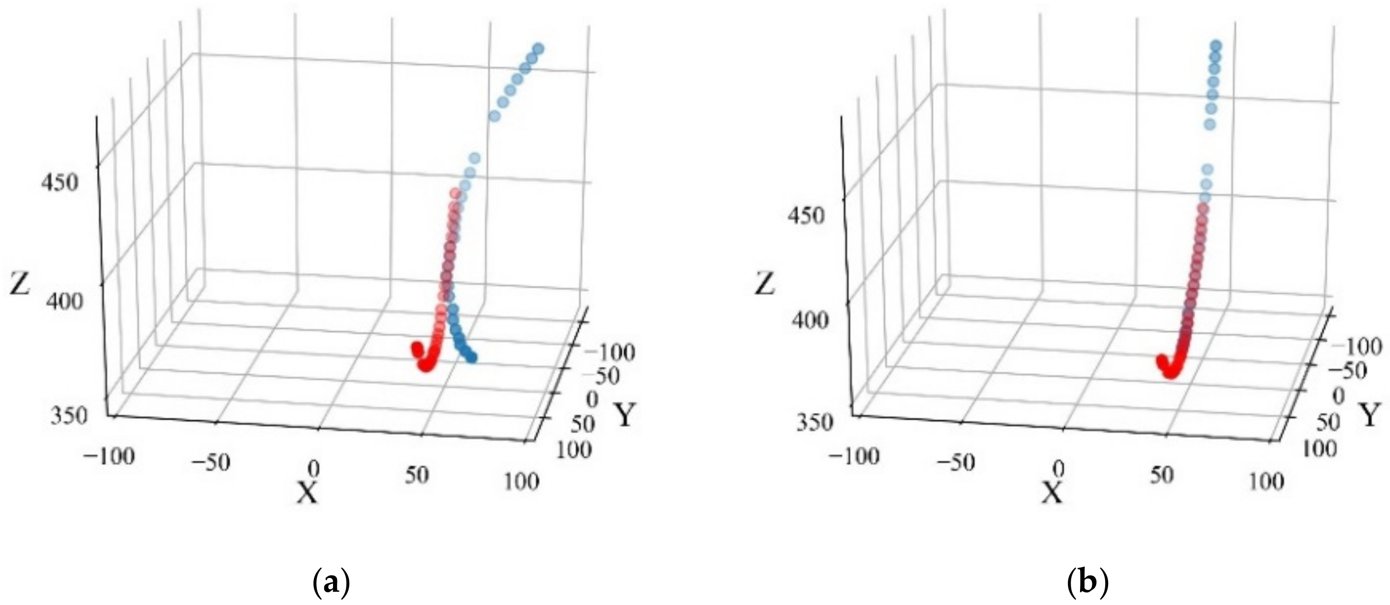
Figure 14a shows the effect of using the traditional SVD algorithm to solve the transformation. It is not difficult to see that the registration of the two groups of point clouds has not achieved the expected effect, and there is an obvious angle difference between the planes where they are located. After applying the improvements proposed in this paper, it is clearly found from Figure 14b that the matching effect is better at this time. The two groups of point clouds have a small error between points, and their plane normal vectors are also almost parallel.
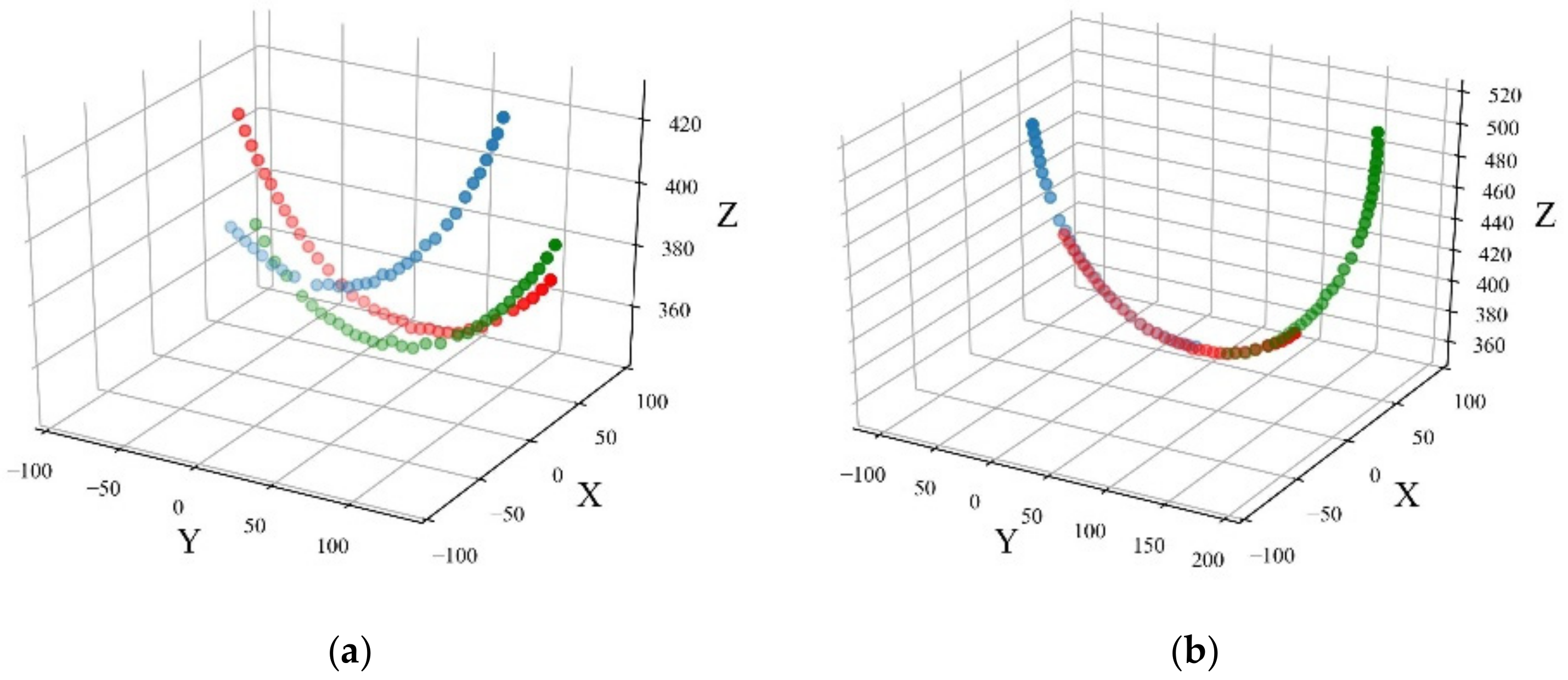
During the measurement of the pipe section illustrated in Figure 11, three sets of binocular cameras generate three feature point clouds that were not given in the same coordinate system. To reduce the error generated in the point-cloud-registration process, the three sets of point clouds are all converted to the coordinate system based on the second set of point clouds, and the integration result is shown in Figure 15. Figure 15a shows the three sets of original point clouds before point-cloud registration. After point-cloud registration, the semicircular arc shown in Figure 15b is generated, which proves the effectiveness of the point-cloud-registration algorithm.
3.3. Validation Experiment
In the validation experiment, a seamless steel pipe is used as the test object, and ten cross sections of the pipe are taken for diameter measurement. The single measurement value of the CMM is used as the reference. In this experimental system, the average of five measurements is taken as the final measurement. The validation-experiment results are shown in Table 1.
By analyzing the experimental results, we find that in the measurements of ten cross sections, the maximum absolute error and the average absolute error are −1.71 mm and 0.847 mm, respectively. The relative error is within ±0.570%, which is close to the result of typical manual measurement with a tape.
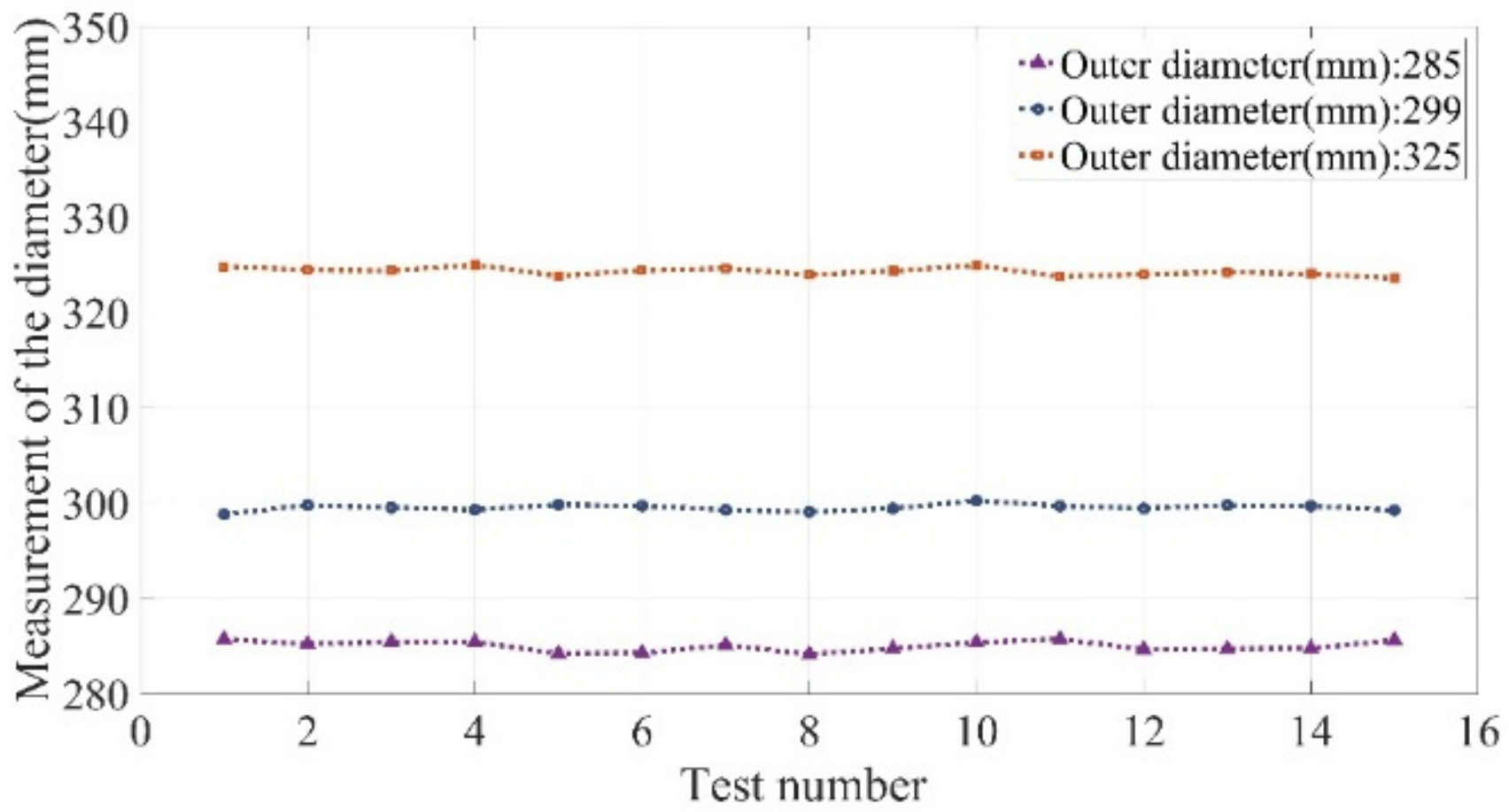
To analyze the repeatability in measurement, we use common seamless steel pipes with outer diameters of 285 mm, 299 mm, and 325 mm for replicated tests. For each steel pipe, a cross section is selected and measured 15 times. The final measurement results are shown in Figure 16.
It is seen from the results that the maximum absolute error, i.e., the largest difference between a measurement and an average, is 0.865 mm, 0.724 mm, and 0.715 mm, respectively, for the three types of steel pipes. Based on calculation with the Bessel formula, the diameter-measurement repeatability standard deviations of the three types of pipes measured by this experimental system are 0.551 mm, 0.356 mm, and 0.428 mm, respectively. In general, the system exhibits good measurement repeatability. The maximum repeatability standard deviation is 0.551 mm for pipes in the diameter range from 285 mm to 325 mm, thus meeting practical needs.
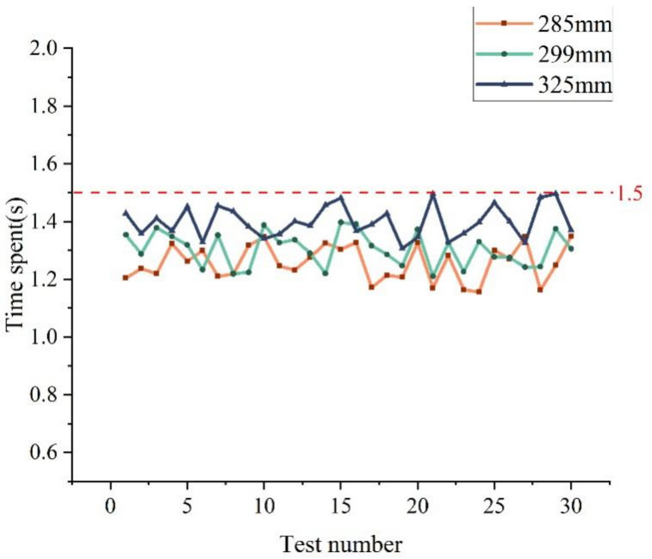
To analyze the measurement efficiency of the experimental system, a total of 90 measurements were made on the three types of pipes mentioned above, and the time consumption of the measurements was recorded. The result is shown in Figure 17, and it is found that the average measurement times for the three types of pipes are 1.262 s, 1.305 s, and 1.391 s, and the maximum measurement time is 1.495 s.
4. Conclusions
To address existing practical problems in today’s large-sized-pipe-measurement methods, this paper proposes a unique solution and builds an experimental system to verify the proposed solution. The experimental results show that compared with the data measured by CMM, the relative error of the proposed measurement system is within ±0.570% and the maximum absolute error is −1.71 mm. In replicated tests, the maximum repeatability standard deviation of the three sizes of steel pipes (285 mm, 299 mm, and 325 mm) is 0.551 mm. While guaranteeing high precision, the proposed measurement algorithm provides a stable running cycle of about 1.5 s, which meets the needs for pipe measurement in actual production applications. In conclusion, this method enables fast in situ measurement of large-sized pipes at high precision, and therefore has broad application prospects.
Author Contributions
Conceptualization, P.L. and L.Z.; methodology, P.L. and L.Z.; software, P.L. and M.W.; validation, P.L., L.Z. and M.W.; formal analysis, P.L. and M.W.; investigation, P.L. and M.W.; resources, L.Z.; data curation, P.L.; writing—original draft preparation, P.L. and L.Z.; writing—review and editing, P.L. and M.W.; visualization, P.L. and L.Z.; supervision, M.W.; project administration, L.Z.; funding acquisition, L.Z. and M.W. All authors have read and agreed to the published version of the manuscript.
Funding
This research was funded by the National Natural Science Foundation of China (Grant No. 61905220), the Natural Science Foundation of Zhejiang Province (Grant No. LGF21F050004), and the Zhejiang Provincial Department of Education Scientific Research Project (Grant No. 20020059-F).
Data Availability Statement
The data that support the findings of this study are available from the corresponding authors upon reasonable request.
Acknowledgments
The authors thank the editors and anonymous reviewers for providing helpful suggestions for improving the quality of this manuscript.
Conflicts of Interest
The authors declare no conflict of interest.
References
- Hashmi, M.S.J. Aspects of tube and pipe manufacturing processes: Meter to nanometer diameter. J. Mater. Processing Technol. 2006, 179, 5–10. [Google Scholar] [CrossRef]
- Yang, Z.; Tian, W.; Ma, Q.; Li, Y.; Li, J.; Gao, J.; Zhang, H.; Yang, Y. Mechanical properties of longitudinal submerged arc welded steel pipes used for gas pipeline of offshore oil. Acta Metall. Sin. 2008, 21, 85–93. [Google Scholar] [CrossRef]
- Diogo, A.F.; Vilela, F.A. Head losses and friction factors of steady turbulent flows in plastic pipes. Urban Water J. 2014, 11, 414–425. [Google Scholar] [CrossRef]
- Safdarian, R. Experimental and numerical investigation of wrinkling and tube ovality in the rotary draw bending process. Proc. Inst. Mech. Eng. Part C J. Mech. Eng. Sci. 2019, 233, 5568–5584. [Google Scholar] [CrossRef]
- Mekid, S.; Vacharanukul, K. In–process out–of–roundness measurement probe for turned workpieces. Measurement 2011, 44, 762–766. [Google Scholar] [CrossRef]
- Schöch, A.; Salvadori, A.; Germann, I.; Balemi, S.; Bach, C.; Ghiotti, A.; Carmignato, S.; Maurizio, A.L.; Savio, E.; Ag, Z.E.; et al. High–speed measurement of complex shaped parts at elevated temperature by laser triangulation. Int. J. Autom. Technol. 2015, 9, 558–566. [Google Scholar] [CrossRef]
- Zhang, Y.; Wang, Y.; Liu, Y.; Lv, D.; Fu, X.; Zhang, Y.; Li, J. A concentricity measurement method for large forgings based on laser ranging principle. Measurement 2019, 147, 106838. [Google Scholar] [CrossRef]
- Zhang, Y.C.; Miao, S.; Fu, X.B.; Li, Q.; Gao, J.H. Online measuring method of radial section line for ring forgings. Int. J. Adv. Manuf. Technol. 2019, 101, 3035–3046. [Google Scholar] [CrossRef]
- Cavedo, F.; Norgia, M.; Pesatori, A.; Solari, G.E. Steel pipe measurement system based on laser rangefinder. IEEE Trans. Instrum. Meas. 2016, 65, 1472–1477. [Google Scholar] [CrossRef]
- Fu, X.; Zhang, Y.; Tao, K.; Li, S. The outer diameter detection and experiment of the circular forging using laser scanner. Optik 2017, 128, 281–291. [Google Scholar] [CrossRef]
- Fu, X.; Liu, B.; Zhang, Y. An optical non–contact measurement method for hot–state size of cylindrical shell forging. Measurement 2012, 45, 1343–1349. [Google Scholar] [CrossRef]
- Du, Z.; Du, Y. Simple three–dimensional laser radar measuring method and model reconstruction for hot heavy forgings. Opt. Eng. 2012, 51, 021118. [Google Scholar] [CrossRef]
- Ayub, M.A.; Mohamed, A.B.; Esa, A.H. In–line inspection of roundness using machine vision. Procedia Technol. 2014, 15, 807–816. [Google Scholar] [CrossRef] [Green Version]
- Xiao, G.; Li, Y.; Xia, Q.; Cheng, X.; Chen, W. Research on the on–line dimensional accuracy measurement method of conical spun workpieces based on machine vision technology. Measurement 2019, 148, 106881. [Google Scholar] [CrossRef]
- Zatočilová, A.; Paloušek, D.; Brandejs, J. Image–based measurement of the dimensions and of the axis straightness of hot forgings. Measurement 2016, 94, 254–264. [Google Scholar] [CrossRef]
- Zhou, Y.; Wu, Y.; Luo, C. A fast dimensional measurement method for large hot forgings based on line reconstruction. Int. J. Adv. Manuf. Technol. 2018, 99, 1713–1724. [Google Scholar] [CrossRef]
- Quentin, L.; Beermann, R.; Pösch, A.; Reithmeier, E.; Kästner, M. 3D geometry measurement of hot cylindric specimen using structured light[C]//Optical Measurement Systems for Industrial Inspection X. Int. Soc. Opt. Photonics 2017, 10329, 103290U. [Google Scholar] [CrossRef] [Green Version]
- Bračun, D.; Škulj, G.; Kadiš, M. Spectral selective and difference imaging laser triangulation measurement system for on line measurement of large hot workpieces in precision open die forging. Int. J. Adv. Manuf. Technol. 2017, 90, 917–926. [Google Scholar] [CrossRef]
- Rahayem, M.; Werghi, N.; Kjellander, J. Best ellipse and cylinder parameters estimation from laser profile scan sections. Opt. Lasers Eng. 2012, 50, 1242–1259. [Google Scholar] [CrossRef]
- Zhang, Y.C.; Luo, C.; Fu, X.B.; Chen, Y.M. Automatic measurement method for the size of large forgings based on scattering on rough surface. IET Sci. Meas. Technol. 2017, 11, 118–124. Available online: https://0-ietresearch-onlinelibrary-wiley-com.brum.beds.ac.uk/doi/pdfdirect/10.1049/iet-smt.2016.0283 (accessed on 20 January 2022). [CrossRef]
- Zhang, Y.C.; Han, J.X.; Fu, X.B.; Zhang, F.L. Measurement and control technology of the size for large hot forgings. Measurement 2014, 49, 52–59. [Google Scholar] [CrossRef]
- Matsui, K.; Yamashita, A.; Kaneko, T. 3–d shape measurement of pipe by range finder constructed with omni–directional laser and omni–directional camera. In Proceedings of the 2010 IEEE International Conference on Robotics and Automation, Anchorage, AK, USA, 3–7 May 2010; pp. 2537–2542. [Google Scholar] [CrossRef]
- Lee, H.W.; Hsu, P.E.; Pan, S.P.; Liu, T.A.; Liou, H.C. Applying Structured Light on Cylinder Straightness Detection Using Break Line Method. In Applied Mechanics and Materials; Trans Tech Publications Ltd.: Bäch SZ, Switzerland, 2015; Volume 764, pp. 1298–1303. Available online: https://0-doi-org.brum.beds.ac.uk/10.4028/www.scientific.net/AMM.764-765.1298 (accessed on 1 February 2022). [CrossRef]
- Sansoni, G.; Bellandi, P.; Docchio, F. Design and development of a 3D system for the measurement of tube eccentricity. Meas. Sci. Technol. 2011, 22, 075302. [Google Scholar] [CrossRef] [Green Version]
- Lu, R.S.; Li, Y.F.; Yu, Q. On–line measurement of the straightness of seamless steel pipes using machine vision technique. Sens. Actuators A Phys. 2001, 94, 95–101. [Google Scholar] [CrossRef]
- Jia, Z.; Wang, L.; Liu, W.; Yang, J.; Liu, Y.; Fan, C.; Zhao, K. A field measurement method for large objects based on a multi–view stereo vision system. Sens. Actuators A Phys. 2015, 234, 120–132. [Google Scholar] [CrossRef]
- Jia, Z.; Liu, Y.; Liu, W.; Zhang, C.; Yang, J.; Wang, L.; Zhao, K. A spectrum selection method based on SNR for the machine vision measurement of large hot forgings. Optik 2015, 126, 5527–5533. [Google Scholar] [CrossRef]
- Liu, Y.; Jia, Z.; Liu, W.; Wang, L.; Fan, C.; Xu, P.; Yang, J.; Zhao, K. An improved image acquisition method for measuring hot forgings using machine vision. Sens. Actuators A Phys. 2016, 238, 369–378. [Google Scholar] [CrossRef]
Figure 1.
Schematic diagram of the proposed measurement system.

Figure 2.
Flow chart of measurement algorithm.

Figure 3.
Principle of binocular vision.

Figure 4.
Schematic diagram of affine distance transformation.

Figure 5.
Laser markers distribution.

Figure 6.
Feature point matching flowchart.

Figure 7.
Flow chart of point-cloud registration.

Figure 8.
Schematic diagram of point-cloud registration.

Figure 9.
Fitting-error distribution for diameter.

Figure 10.
(a) The experimental system built in this paper; (b) coordinate measuring machine for reference.
Figure 10.
(a) The experimental system built in this paper; (b) coordinate measuring machine for reference.

Figure 11.
(a) Extraction of feature points for left camera; (b) extraction of feature points for right camera.
Figure 11.
(a) Extraction of feature points for left camera; (b) extraction of feature points for right camera.

Figure 12.
Feature-point-matching elements.

Figure 13.
Feature-point-matching results.

Figure 14.
(a) Estimation results by SVD; (b) estimation results by the improved algorithm.

Figure 15.
(a) Raw point clouds; (b) point clouds after registration.

Figure 16.
Replicate test results of pipe diameter.

Figure 17.
Time-consumption-record results.


Table 1.
Validation-experiment results.
| Cross Section Number | 1 | 2 | 3 | 4 | 5 | 6 | 7 | 8 | 9 | 10 |
|---|---|---|---|---|---|---|---|---|---|---|
| CMM (mm) | 299.514 | 299.501 | 299.494 | 299.493 | 299.493 | 299.500 | 299.545 | 299.167 | 299.512 | 299.514 |
| This article (mm) | 298.454 | 298.565 | 298.790 | 299.255 | 300.586 | 299.355 | 297.837 | 298.561 | 298.185 | 300.171 |
| Absolute error (mm) | −1.06 | −0.936 | −0.704 | −0.238 | 1.09 | −0.145 | −1.71 | −0.606 | −1.33 | 0.657 |
| Relative error (%) | −0.354 | −0.313 | −0.235 | −0.0790 | 0.365 | −0.0480 | −0.570 | −0.203 | −0.443 | 0.219 |
Publisher’s Note: MDPI stays neutral with regard to jurisdictional claims in published maps and institutional affiliations. |
© 2022 by the authors. Licensee MDPI, Basel, Switzerland. This article is an open access article distributed under the terms and conditions of the Creative Commons Attribution (CC BY) license (https://creativecommons.org/licenses/by/4.0/).
Share and Cite
MDPI and ACS Style
Liu, P.; Zhang, L.; Wang, M. Measurement of Large-Sized-Pipe Diameter Based on Stereo Vision. Appl. Sci. 2022, 12, 5277. https://0-doi-org.brum.beds.ac.uk/10.3390/app12105277
AMA Style
Liu P, Zhang L, Wang M. Measurement of Large-Sized-Pipe Diameter Based on Stereo Vision. Applied Sciences. 2022; 12(10):5277. https://0-doi-org.brum.beds.ac.uk/10.3390/app12105277
Chicago/Turabian StyleLiu, Pu, Lieshan Zhang, and Meibao Wang. 2022. "Measurement of Large-Sized-Pipe Diameter Based on Stereo Vision" Applied Sciences 12, no. 10: 5277. https://0-doi-org.brum.beds.ac.uk/10.3390/app12105277
Note that from the first issue of 2016, this journal uses article numbers instead of page numbers. See further details here.