
An Intelligent Optimization Back-Analysis Method for Geomechanical Parameters in Underground Engineering

1
Guangxi Xinfazhan Transportation Group Co., Ltd., Nanning 530004, China
2
Key Laboratory of Disaster Prevention and Structural Safety of Ministry of Education, College of Civil Engineering and Architecture, Guangxi University, Nanning 530004, China
3
Guangxi Provincial Engineering Research Center of Water Security and Intelligent Control for Karst Region, Guangxi University, Nanning 530004, China
4
Guangxi Key Laboratory of Geomechanics and Geotechnical Engineering, College of Civil Engineering and Architecture, Guilin University of Technology, Guilin 541004, China
*
Author to whom correspondence should be addressed.
Appl. Sci. 2022, 12(11), 5761; https://0-doi-org.brum.beds.ac.uk/10.3390/app12115761
Submission received: 20 April 2022
/
Revised: 2 June 2022
/
Accepted: 3 June 2022
/
Published: 6 June 2022
(This article belongs to the Section Civil Engineering)
Abstract
:The geomechanical parameters in underground engineering are usually difficult to determine, which can pose great obstacles in underground engineering. A novel displacement back-analysis method is proposed to determine the geomechanical parameters in underground engineering. In this method, the problem of geomechanical parameter determination is converted into an optimization problem, regarding the geomechanical parameters as the optimization parameters, and the error between the calculated results and the field measurement information as the optimization objective function. The grasshopper optimization algorithm (GOA), which offers excellent global optimization performance, and the Gaussian process regression (GPR) machine learning, offering powerful fitting ability, are combined to address the time-consuming numerical calculations. Furthermore, the proposed method is combined with the 3D numerical calculation software FLAC3D to form the GOA-GPR-FLAC3D method, which can be used in the displacement back-analysis of geomechanical parameters in underground engineering. The results of a case study show that the proposed method can greatly improve computational efficiency while ensuring high precision compared with the GOA. When applied to the Tai’an Pumped Storage Power Station, this method can obtain more accurate results compared with the GOA under the same evaluation times and is more suitable for the back-analysis of rock parameters in underground engineering.
1. Introduction
Due to the particularity and complexity of geological conditions in engineering, various rock parameters in underground engineering projects present great uncertainties, which increase difficulties and variables during construction. Although some parameters can be obtained by laboratory tests or in situ tests, due to the size effect, there can be large errors in the parameters, which cannot meet the needs of practical engineering. At present, the rock parameter back-analysis method has become an important means of solving this problem, gradually forming a system of theories and methods that can be used in engineering practice [1,2]. Underground engineering back-analysis is a method that uses displacement, stress, strain and other measured information generated by surrounding rock during underground engineering construction to establish a model and carry out numerical simulations to deduce rock parameters and initial load conditions [3,4,5,6]. Displacement information is easier to monitor and obtain than stress data and other measured information, and the displacement back-analysis method is the most widely used method for back-analysis in underground engineering [7,8]. In the displacement back-analysis process, to obtain more practical geomechanical parameters and align the calculated results with field measurement information, the rock parameters are converted to optimization parameters, and the error between the calculated results and the field measurement information is taken as the optimization objective function; this approach is called the optimization back-analysis method.
After decades of research, the optimization of back-analysis methods has been continuously updated and has iteratively injected vitality into the development of the back-analysis field. Traditional optimization methods, such as the simplex method [9], conjugate gradient method [10] and semianalytical method [11], have provided impetus in the initial development of the displacement optimization back-analysis method. However, traditional optimization methods can encounter problems, such as slow convergence speed or weak adaptability, which cannot meet the needs of underground engineering back-analysis [12,13]. Therefore, with the continuous development of the internet and computer technology, some bionic intelligent algorithms, such as the genetic algorithm (GA) [14,15,16], particle swarm optimization (PSO) [17,18,19], and ant colony optimization (ACO) [20], have been gradually introduced into geotechnical engineering and applied in the back-analysis of rock parameters. Since bionic intelligence optimization algorithms are stochastic optimization algorithms, a large number of fitness function evaluations are often required to obtain the global optimal solution for complex optimization problems. However, because the relationship between the parameters and the objective function is difficult to establish through simple formulas, it is generally necessary to use time-consuming numerical calculations to establish the implicit functional relationship, which leads to low computational efficiency and is difficult to apply to engineering practice [21].
In the optimization back-analysis, this problem can be effectively solved by replacing part of the time-consuming numerical calculation with the surrogate model. Genetic algorithm (GA) and artificial neural network (ANN) strategies have been combined to calculate the geomechanical parameters and in situ stresses [22]. When using the back-analysis method to calculate the seepage field parameters of an earth–rock dam, researchers used a support vector machine (SVM) to establish the nonlinear relationship between the seepage parameters and the water head. Then, an objective error function was used as the fitness value of the PSO algorithm, and the seepage parameters were identified by the PSO algorithm [23]. In another study, scholars integrated an orthogonal design method, GA, SVM and numerical simulation software to successfully invert the geomechanical parameters of an underground powerhouse of a large hydropower station [24]. However, for complex nonlinear function problems, ANNs are prone to overfitting and have a slow convergence speed, while SVMs face difficulties in choosing kernel functions and parameters.
In this paper, a novel intelligent algorithm based on the grasshopper optimization algorithm (GOA) and Gaussian process regression (GPR) machine learning is proposed, combining the low computational cost of the GPR surrogate model with the powerful optimization ability of the GOA. On this basis, a back-analysis method called GOA-GPR-FLAC3D is presented through the geotechnical numerical calculation software FLAC3D. Furthermore, the method is applied to a circular tunnel case, and the Tai’an Pumped Storage Power Station, to verify its superiority and practicability in the back-analysis of underground engineering.
2. Related Work
2.1. GOA
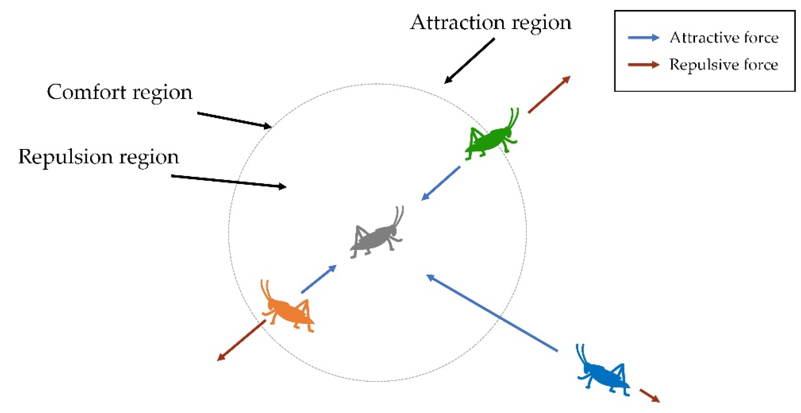
The GOA is an emerging bionic intelligence optimization algorithm that has the characteristics of excellent global optimization capability [25]. The algorithm regards a single individual as a search operator and simulates the wide-ranging fast movements of imagoes and local slow movements of larvae into global and local optimization, respectively. In the optimization process, with an increase in the number of iterations, the global optimization stage gradually transforms into the local optimization stage [26]. In the global optimization stage, the operator performs a rapid search in the model space over a wide range to obtain the general information of the model space and lock down a local area. In the local optimization stage, the operator searches this local area and optimizes the accuracy of the solution through continuous iteration. According to the distance between the two operators, spatial regions can be divided into attractive regions, comfortable regions and repulsive regions (Figure 1).
When the distance between the two operators is relatively close (less than 2.079 units), they repulse each other, and the operator is in the repulsion region or the repulsion distance. When the distance between the two operators is exactly 2.079 units, there is neither an attractive nor repulsive force, which is called the comfort region or the comfortable distance. In the same way, when the distance between two operators is more than 2.079 units, they attract each other, which is called the attraction region or the distance of attraction. According to this principle, grasshopper operators will constantly adjust their positions with other operators to achieve optimized results.
It is important to note that there is no clear boundary between global and local optimization. With increasing iteration times, the search area gradually decreases, and the search gradually changes from global optimization to local optimization. The current grasshopper operator xi is defined by the grasshopper operator xj as follows:
where dij is the spatial distance between the current i-th grasshopper operator and the j-th grasshopper operator; m and n are parameters to evaluate the effect of other agents on the agent, m represents the intensity of attraction, and n represents the spatial scale of attraction.
The next position of the grasshopper operator xi is defined as follows:
where is the position to which the i-th grasshopper operator moves next in the k-th dimension; N represents the total number of grasshopper operators; ulk and flk represent the upper and lower limits of the agent in the k-th dimension, respectively; denotes the spatial distance between the i-th grasshopper and the j-th grasshopper in the k-th dimension; and represent the current position of the i-th and j-th grasshoppers in the k-th dimension, respectively; represents the component of the best solution found thus far in the k-th dimension; and c1 and c2 are known as adaptive shrinkage parameters, which maintain the relative balance between global and local optimization. If c1 and c2 are represented by c, their linear change can be calculated as:
where t represents the current iteration number; tmax represents the maximum number of iterations; cmax is the maximum value of the adaptive shrinkage parameter; cmin is the minimum value of the adaptive shrinkage parameter.
2.2. GPR
Due to the numerous excellent properties of Gaussian distribution, GPR offers good adaptability when dealing with small sample sizes, high dimensions, nonlinearity and other problems [27]. In recent years, GPR has become a trending topic in the field of machine learning [28,29,30].
There are two different ways to derive GPR, which can be explained by weight space and function space. Since the derivation of weight space is deeply dependent on Bayesian theory, this paper specifically explains it from the perspective of weight space for a better understanding.
Let us start with the simplest linear regression model with noise. The formula is shown as follows:
where is the input of dimension p, is the weight vector of dimension p, and y represents the true value. Here, we assume that the noise ε obeys a Gaussian distribution, with 0 as the mean and as the variance. Since we have previous knowledge about the weight vector, it is assumed that it obeys a Gaussian distribution with a mean value of 0 and variance of , namely, .
Through a series of observed training data D = (X,y) = {(xi,yi)|xi∈, yi ∈ R, I = 1,…,n} and the assumption of independent noise distribution, we can calculate the likelihood function as follows:
With the likelihood function and the prior distribution of weights, the posterior distribution of weights can be obtained using a Bayesian formula. First, according to Bayes’ formula:
In the formula, ∝ represents the ignored constant scaling coefficient. In mathematics, the product of two Gaussian density functions is still a Gaussian density function, and the constant scaling coefficient in front of the Gaussian density function does not affect the judgement of the mean and variance of the Gaussian distribution; thus, it can be ignored. Since the denominator after the second equal sign of the above equation is an integral, which results in a constant, the final expression can be obtained by ignoring it.
Substituting the previous calculation of and into the above equation obtains:
where , . According to the form of the Gaussian density function, we can easily determine that it is a multidimensional Gaussian distribution with a mean value and covariance matrix, namely:
With the posterior distribution of this weight, we can predict a group of test points z. Here, we need to use the concept of total probability. is the integral of all possible parameters and their corresponding posterior distribution, that is, the predicted distribution of the predicted value .
If we consider the influence of noise, the predicted distribution of the real value of the final prediction is as follows:
3. GOA-GPR Optimization Algorithm
3.1. Basic Concept
The main strategy of this method is as follows. First, the GOA is used in several rounds of stochastic optimization within the model space. Then, taking the current optimal grasshopper operator as the centre, the 3 × N historical operators closest to the current optimal operator (N is the population number of the GOA algorithm) are obtained to construct the optimization experience dataset. GPR is used to fit the dataset, and the functional relationship between the decision variables and objective function values is constructed to obtain the corresponding surrogate model. Then, the Newton method is used to optimize the surrogate model and obtain the optimal operator of the local region prediction. Because the surrogate model is used to replace the real performance function, the real performance function is not used for fitness evaluation, and the efficient Newton method is used to replace the GOA for local optimization, so the fitness evaluation times of the objective function are significantly reduced and the overall efficiency of the algorithm is improved. Finally, the predictive optimal operator found by the Newton method is substituted into the real objective function to obtain the corresponding fitness value, and the value is compared with the fitness value of the current optimal operator. If it is better than the current optimal operator, the current optimal operator is replaced, and the next round of optimization is conducted. The iterative process does not stop until the convergence criterion is satisfied.
3.2. Methodology
- a.
- GPR model for local area fitting
First, the GOA generates random initialization operators in the model space and performs a real objective function fitness evaluation. After several rounds of global optimization, enough information (location information and fitness information of the grasshopper operator from the optimization process) is obtained in the model space, and then the obtained information is used to construct the empirical dataset. The general strategy of construction is as follows: Select an optimal operator as the current optimal operator from all the acquired operators and select the operators close to the current optimal operator to construct the empirical dataset. Finally, GPR is used to fit the samples in the dataset to establish the functional relationship between the decision variables and objective function values to obtain the corresponding surrogate model.
- b.
- Efficient optimization for the surrogate model
Instead of the GOA, the Newton method is used to optimize the local surrogate model. The Newton method uses gradient information to optimize the objective function. Therefore, its computational efficiency is much higher than that of the GOA to improve the overall optimization efficiency of the method.
- c.
- Dynamically updating the empirical dataset for optimization
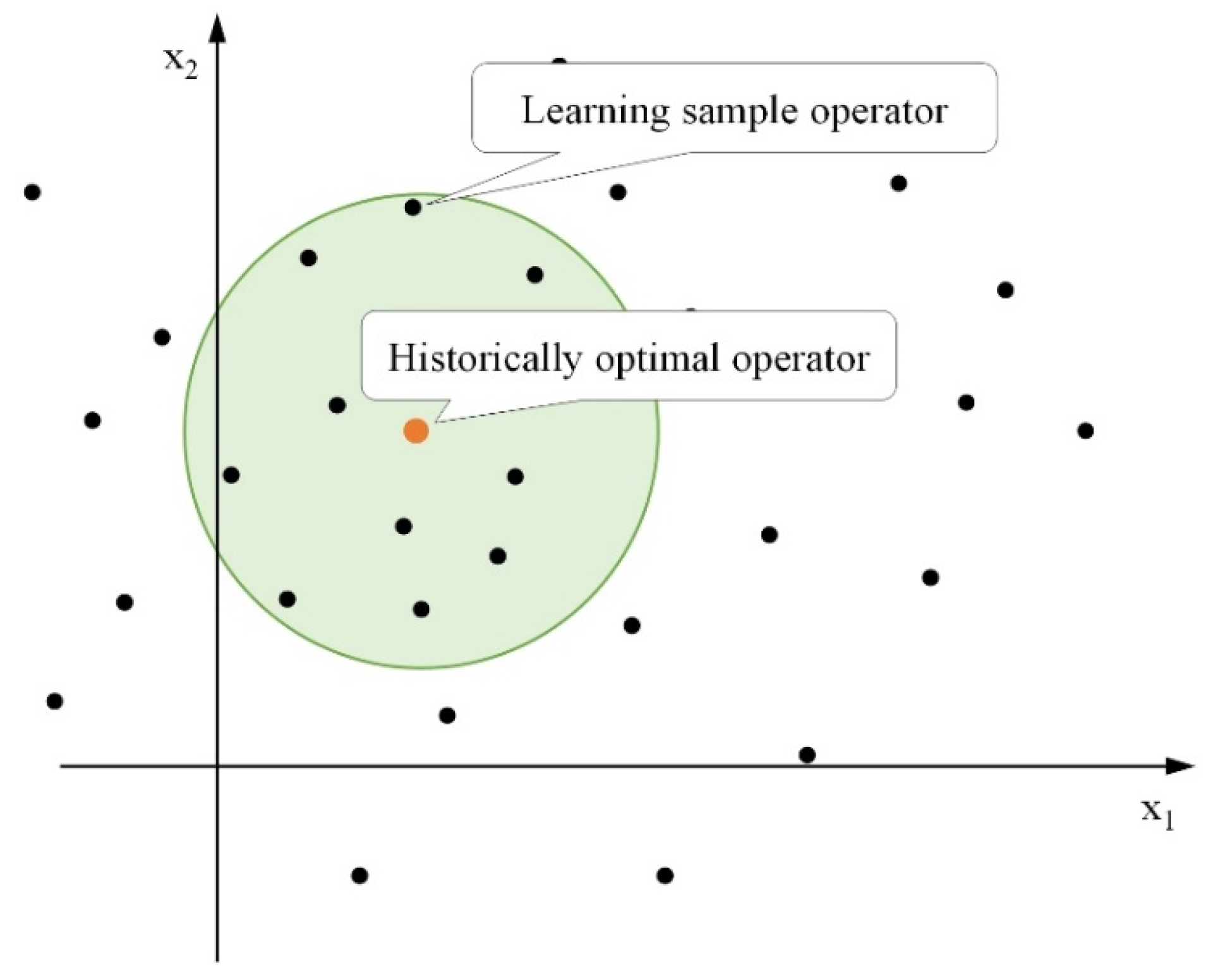
In regression analysis, training samples directly affect the establishment of the surrogate model and ultimately affect prediction accuracy. Therefore, reasonable training samples are very important. In the process of constructing the optimization experience dataset, we need to constantly dynamically adjust the optimization experience dataset and optimize the training samples in the experience dataset to give full play to the surrogate model. The main implementation steps for dynamically updating the empirical optimization dataset are as follows: In the previous rounds of global optimization, a historical dataset containing all operator information is constructed, which records all historical positions and corresponding fitness values of operators in the optimization process. Before local area optimization, the empirical dataset is established based on the historical information dataset. As shown in Figure 2, operators in local areas are used in this paper to construct the empirical optimization dataset. Taking the current optimal operator as the centre, the operator nearest to the centre is selected to construct the empirical optimization dataset. In the optimization process, by keeping the total number of operators in the dataset unchanged and dynamically adjusting the location of the centre point, the optimization dataset is constantly optimized to improve the accuracy and final prediction performance of the surrogate model.
3.3. Procedures
The proposed method can be implemented through the following steps.
- Step 1: Initialize the GOA and GPR parameters. In the model space, N spatial positions are randomly selected as the initial positions of the grasshopper operator. The fitness of each operator is evaluated, and global optimization is performed by the GOA program. After several rounds of global optimization, the current optimal operator is found, and several rounds of all optimization operators in the location information process and corresponding fitness values are saved to the historical dataset. During these rounds of global optimization, determine whether the optimization results meet the convergence criteria. If so, stop the iteration and proceed to Step 7. Otherwise, go to Step 2.
- Step 2: Taking the current optimal operator as the centre point, the operator nearest to the centre point is selected from the historical dataset to construct the empirical dataset of optimization.
- Step 3: GPR is used to fit the samples in the optimization empirical dataset to establish the functional relationship between the decision variables and objective function values to obtain the corresponding surrogate model.
- Step 4: Solve the first and second derivative information of the GPR surrogate model (approximate fitness function). An initial point is randomly selected in the model space of the surrogate model. The corresponding first and second derivatives are obtained, and the iterative formula of Newton’s method is used for iterative optimization. When the gradient value is lower than the preset threshold value, it is considered to reach the extreme point, and the optimal prediction operator is obtained.
- Step 5: The optimal prediction operator is substituted into the real objective function to obtain the corresponding fitness value, and the information of the operator is recorded in the historical dataset.
- Step 6: If the fitness value of the optimal predictive operator is better than that of the current optimal operator, the information of the optimal predictive operator is used to replace the information of the current optimal operator. At the same time, judge whether the current optimal operator meets the convergence criterion. If so, stop the iteration and go to Step 7. Otherwise, go to Step 2.
- Step 7: Output the information of the current optimal operator.
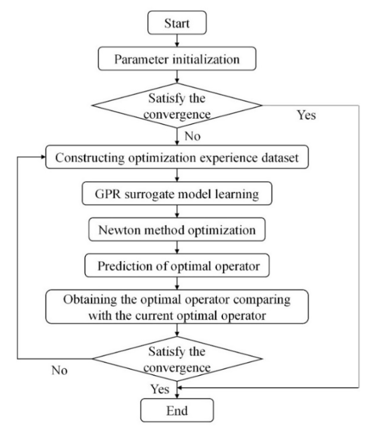
The flowchart of the method is shown in Figure 3.
4. Results and Discussion
To verify the feasibility of this method, two sets of mathematical test functions with optimal solutions are given, including a multipeak test function and a composite test function.
4.1. Case 1
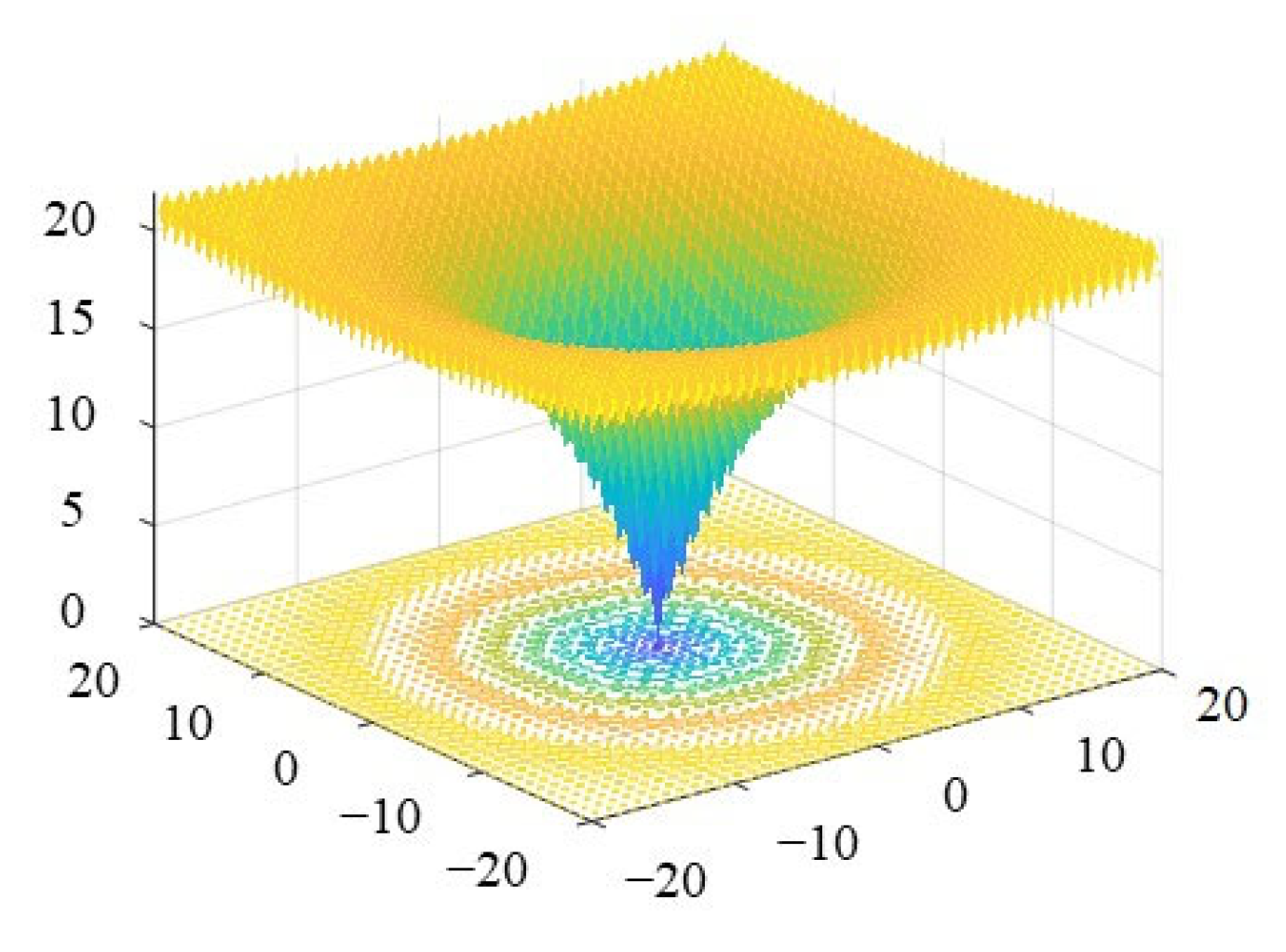
A multipeak test function is given as follows:
where the range is [−32, 32]; the optimal solution fmin is 0. The three-dimensional space surface diagram of the function is shown in Figure 4.
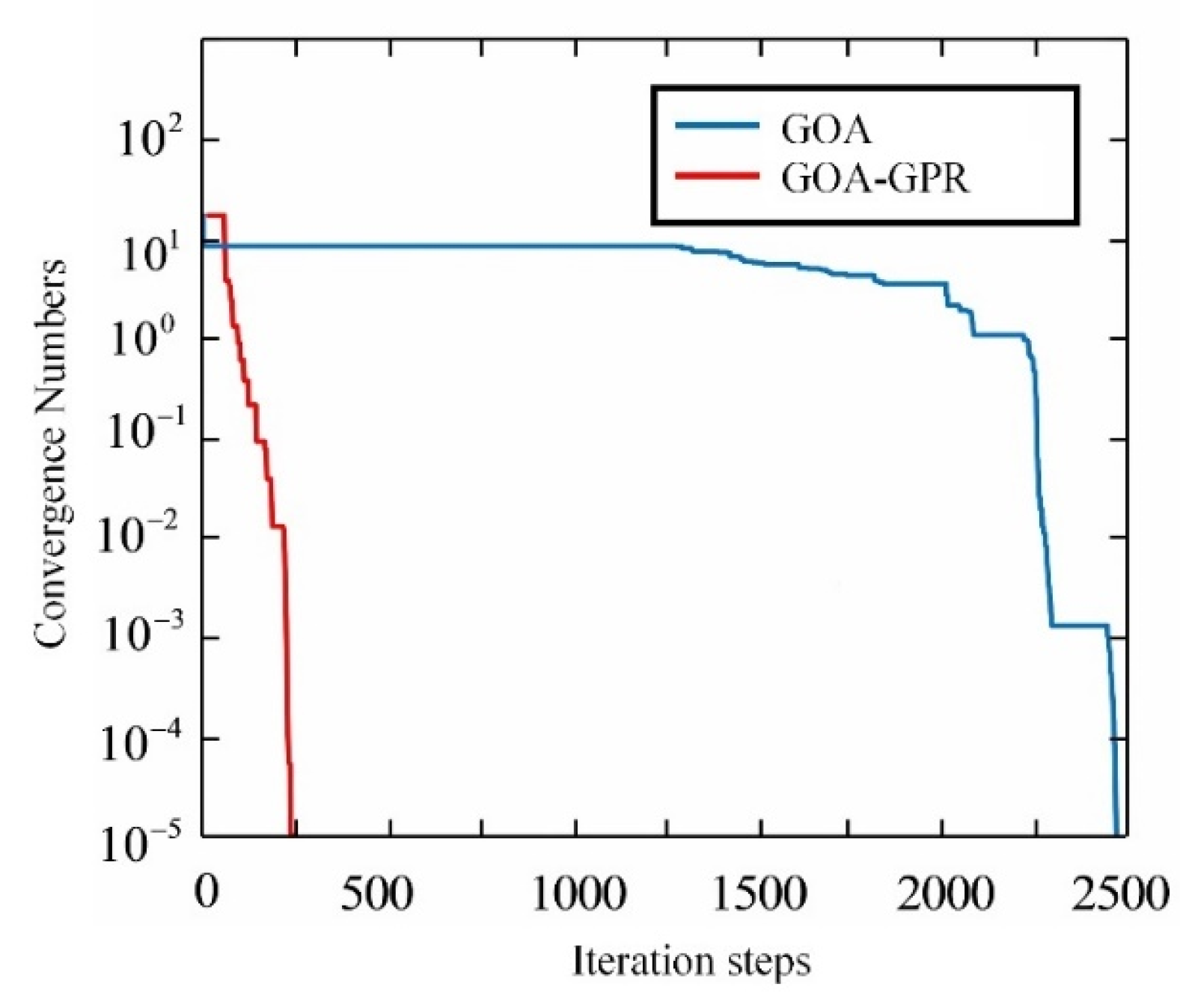
The parameter settings of the GOA are as follows: the dimension D is 30; N is 150; cmax is 1.0, and cmin is 1.0 × 10⁻⁵. The parameter settings of the GPR algorithm are as follows: lnl = [−1, −1]15, lnσf = −1, σn = 1 × 10⁻⁶. The test calculation results between the GOA and GOA-GPR algorithm are shown in Table 1. The convergence curve of the test function is shown in Figure 5. As seen in the table and figure, the average number of function evaluations of the GOA is 10 times that of the GOA-GPR algorithm.
4.2. Case 2
A composite test function is given as follows:
where the value range is [−100, 100]; the optimal solution fmin is 0. The three-dimensional space surface diagram of the function is shown in Figure 6.
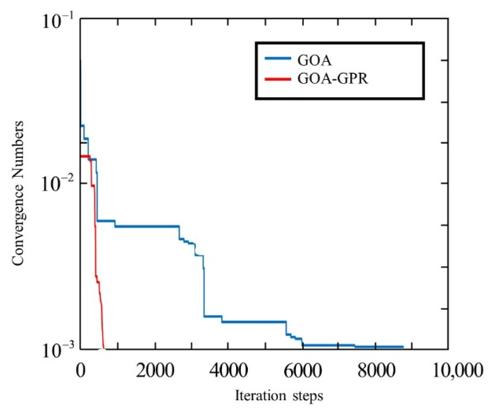
The parameter settings of the GOA are as follows: D is 5; N is 50; cmax is 1.0; cmin is 1.0 × 10⁻⁵. The parameter settings of the GPR algorithm are as follows: lnl = [−1, −1]15, lnσf = −1, σn = 1 × 10⁻⁶. The test calculation results between the GOA and GOA-GPR algorithm are shown in Table 2. The convergence curve of the test function is shown in Figure 7. For the complex composite test functions, the average function evaluation times of the GOA-GPR algorithm are 12 times those of the GOA. Compared with the GOA, the GOA-GPR algorithm proposed in this paper can significantly reduce the evaluation times of the objective function, and the convergence speed is fast, which provides a theoretical possibility for the application of the GOA-GPR algorithm to complex rock mechanics optimization problems.
5. Back-Analysis of Rock Parameters with GOA-GPR-FLAC3D
5.1. Proposed Method
The optimization back-analysis of displacement finds the best combination of parameters by iterative optimization and makes the calculated displacement value approach the measured displacement value step-by-step while correcting the parameters to be determined. The objective function of the optimization back-analysis of displacement can be set in the following form:
where X is a set of parameters to be inverted; di(X) is the calculated displacement value of the first monitoring point on the rock and soil mass; is the measured displacement value of the i-th monitoring point; n is the number of total displacement monitoring points. The essence of an objective function is the mean square error (MSE) that reflects displacement. The ultimate goal of the optimization back-analysis of displacement is to find a set of rock mechanical parameters X so that the value of the objective function can be minimized, and the parameter X corresponding to the minimum value can be considered the “equivalent mechanical parameter” of the on-site rock.
FLAC3D, which was first developed by Itasca Consulting Group, Inc. in Minneapolis, Minnesota, the United States, is a numerical analysis software based on the three-dimensional explicit finite difference method. FLAC3D is widely used in mechanical calculations in the field of geotechnical engineering due to its wide application range, simple embedded language and powerful pre- and post-processing functions. An optimization back-analysis method that combines the GOA-GPR cooperative optimization algorithm with the FLAC3D numerical method is proposed in this section and as GOA-GPR-FLAC3D. This method integrates the FLAC3D program into the GOA-GPR cooperative optimization algorithm and provides a new method for the back-analysis of geomechanical parameters.
The specific implementation steps of the algorithm in this section are as follows:
- Step 1: Initialize the parameters of the GPR model and determine the value range of the geomechanical parameters.
- Step 2: Within the parameter value range, the GOA is used to randomly generate N initialization operators with parameters, and the FLAC3D software is used to calculate the corresponding objective function value of the initial operator to obtain the fitness value of the initial operator. Then, determine whether the grasshopper operator in the historical value set satisfies the convergence criterion. If so, output the corresponding operator information; otherwise, go to Step 3.
- Step 3: During the GOA global optimization process, all the operator information is recorded in the historical database.
- Step 4: In the historical dataset, the current optimal operator is selected, and 3 × N optimal operators are selected from the entire historical dataset to construct a global optimization experience dataset.
- Step 5: GPR is used to model the global optimization experience set and solve the first and second derivative information of the GPR approximate fitness function at the same time. An initial point is randomly selected within the parameter value range of the surrogate model, and the iterative formula of Newton’s method is used for iterative optimization. When the gradient value is lower than the preset threshold value, that is, the extreme point is reached, then the optimal prediction operator is obtained.
- Step 6: Substitute the predicted optimal operator into the FLAC3D program to evaluate the real fitness function and compare it with the fitness value of the current optimal operator. If the fitness value of the predicted optimal operator is better than the current optimal operator, use the predicted optimal operator information to replace the current optimal operator information; otherwise, do not replace it.
- Step 7: Determine whether the current optimal operator satisfies the convergence criterion. If so, stop the optimization and output the current optimal operator information; otherwise, go to Step 2.
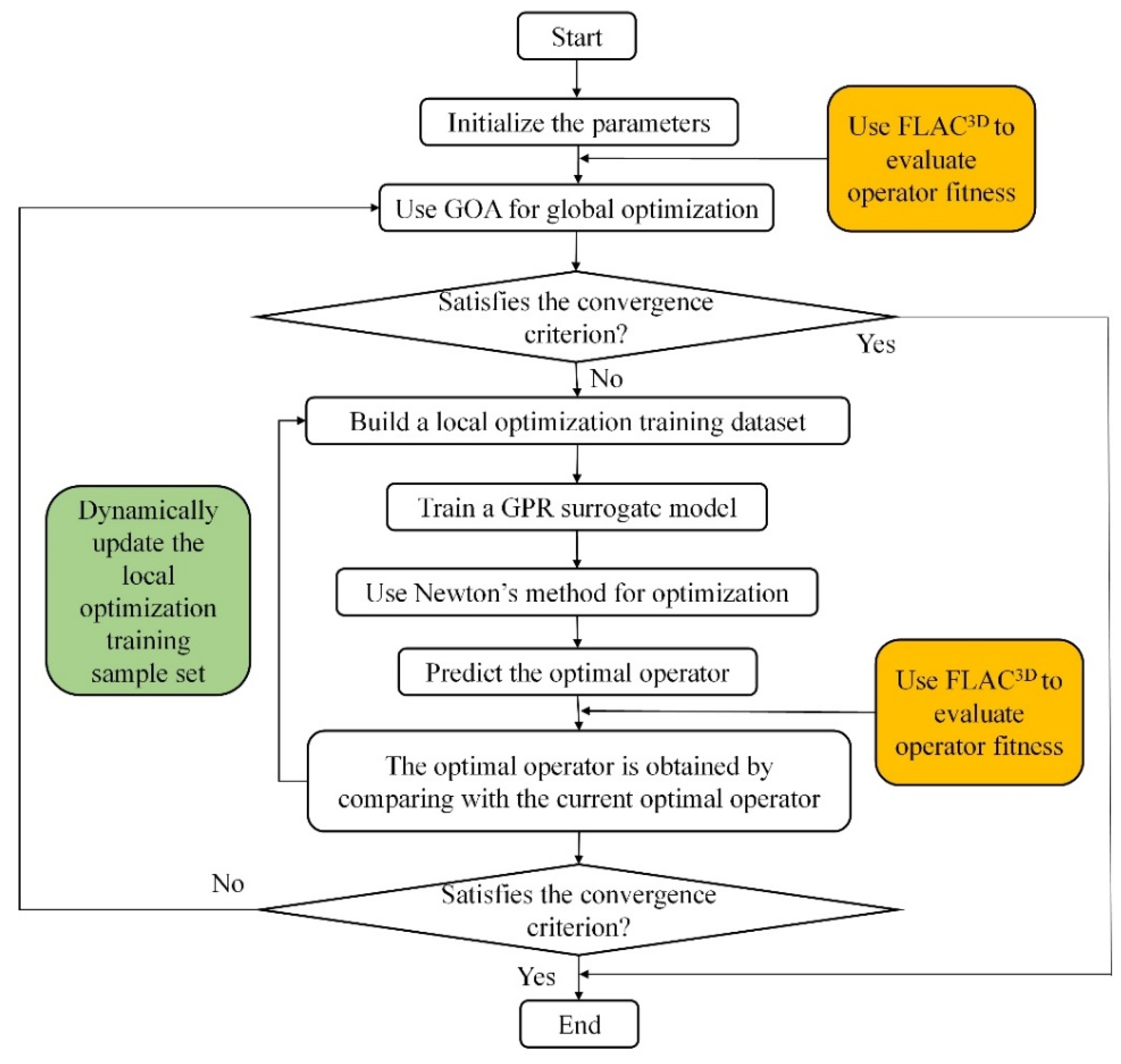
According to the steps described above, the flowchart of the method is shown in Figure 8.
5.2. Case Study
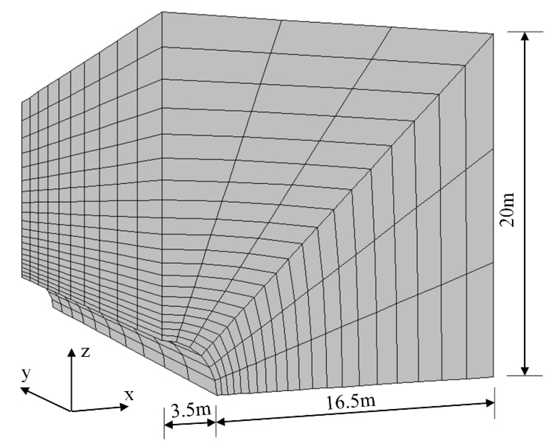
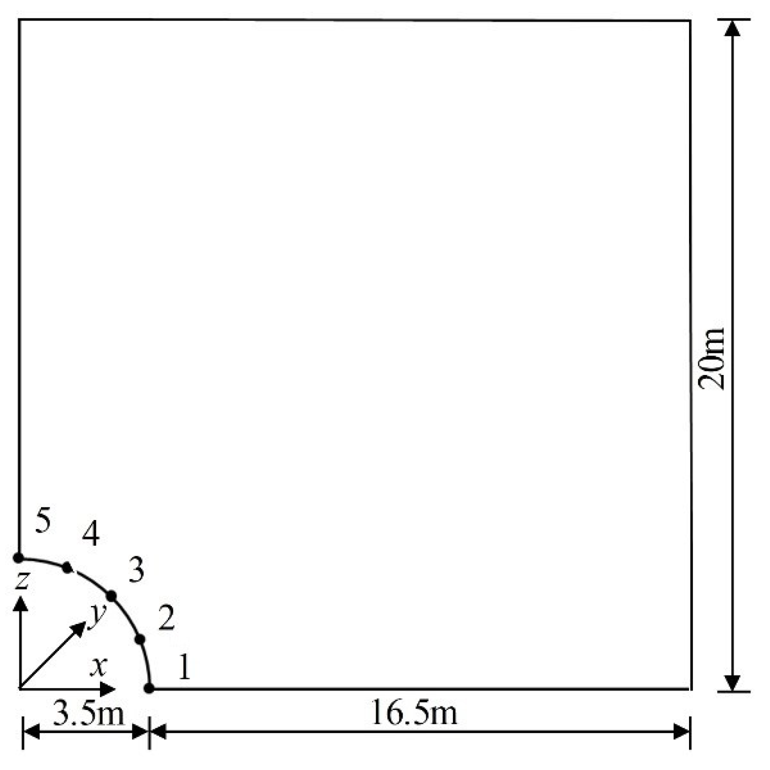
Taking a quarter circular tunnel as an example, a back-analysis of rock mechanical parameters is carried out. The tunnel radius is 3.5 m; the thickness of the tunnel surrounding rock in the x-direction and z-direction is 16.5 m; the buried depth of the tunnel is 50 m; the bulk density of the surrounding rock is 2000 kg/m3; the initial in situ stress field in the rock is mainly composed of a gravity stress field, and the initial in situ stress is σ0 = 10 MPa. In this case, the classic Mohr–Colomb elastoplastic constitutive model is adopted. The ideal elastic–plastic constitutive model based on the Mohr–Colomb failure criterion is one of the most widely used constitutive models in the field of rock engineering [31]. The model has few input parameters and can well describe the mechanics of surrounding rock after underground engineering excavation, and can be used to distinguish whether rock mass is fractured according to whether the grid element of numerical calculation has entered the plastic state. The elastic modulus, cohesion and internal friction angle need to be inversely analysed.
In the FLAC3D software, the generated Lagrangian finite volume mesh covers the entire physical region that needs to be analysed. The smallest meshes may contain only one element, but most are defined by meshes of hundreds, thousands or even millions of elements [32]. Users generally control the grid to adapt to various shapes of 3D problem domains by matching and connecting the built-in grid generator. Figure 9 shows the division of the tunnel mesh. The tunnel model used a hexahedron with 8-nodes and 6-quadrilateral faces as the finite difference element body, which is called a zone in FLAC3D. Through the mesh prototype library that comes with the software, the embedded cylindrical radial-gradient rectangular mesh required for this case was directly generated. The adopted grid was composed of 1000 zones with 1386 grid points. The size and density settings of the grid elements were based on the adopted methods [33,34], considering the surrounding rock properties, strain and integration technique (implicit or explicit). The closer it is to the excavation surface, the smaller the mesh scale is. Multiple computational models with a grid density from small to large were compared. When the mesh density was increased, the change in the calculation results was small, and the correspondingly finer mesh was used.
In the process of the FLAC3D calculation and simulation, the boundary conditions can be divided into two categories: stress boundary conditions and displacement boundary conditions [35]. The boundary referred to here can be the real boundary that actually exists in the real situation, or it can be the artificial boundary assumed by the user in order to make the model closed. Displacement boundary conditions cannot be set directly in FLAC3D. In order to apply a known displacement value to the boundary, it is necessary to define the velocity value at the boundary when the calculation reaches the specified number of steps. In this case, since the tunnel model only simulates a small part of the surrounding rock, the displacement boundary of the model needs to be constrained to prevent the model from large deformation at the artificial boundary. The specific displacement boundary conditions defined by adopting the penalty method [36,37] were as follows: the bottom surface of the model was constrained along the z-direction; the left and right surfaces were constrained along the x-direction, and the front and rear surfaces were constrained along the y-direction. Gradient stress was applied to the entire model from the top of the model along the direction of gravity to simulate the in situ stress of surrounding rock as the stress boundary condition. In order to carry on the proper analysis of the tunnel excavation process, it was necessary to divide the shallow tunnel excavation process into four subsequent sub-steps as follows:
- Step 1: The classical elastic solution method was adopted to ensure the stability of the in situ stress solution. In this method, the constitutive model was set as the elastic model, and the volume modulus and shear modulus were set to large values so that the model could be balanced without plastic failure, and unrealistic displacement or even failure could be prevented.
- Step 2: After confirming the initial in situ stress, the existing displacement and velocity were cleared to zero to avoid interfering with the subsequent analyses. In FLAC3D, accurate calculations are often based on correct initial in situ stress analysis results. Therefore, in the first two steps, the initial in situ stress of the entire model was solved.
- Step 3: The chosen Mohr–Colomb elastoplastic constitutive model described above was assigned to the whole tunnel model and the properties have been changed from elastic to plastic.
- Step 4: The ‘null’ model that comes with FLAC3D was assigned to the part of the grid that needs to be excavated to simulate the actual excavation process.
To verify the feasibility of the algorithm, we assume that the real mechanical parameters of the rock are E = 2.2 GPa, c = 1.1 MPa, φ = 30°. Five monitoring points (1, 2, 3, 4 and 5) are selected at 0°, 22.5°, 45°, 67.5° and 90°, respectively, along the circular direction of the tunnel (see Figure 10). The displacement of the monitoring point (including horizontal displacement and vertical displacement) is calculated by FLAC3D and regarded as the “measured displacement”. The horizontal and vertical displacements calculated by FLAC3D at each monitoring point are shown in Table 3.
For this example, the objective function is:
where di,x and di,z are the calculated displacement components of the horizontal and vertical directions of the i-th monitoring point, respectively; and are the actual displacement components of the horizontal and vertical directions of the i-th monitoring point, respectively; X is a group of decision variables; and the decision variables in this example are elastic modulus E, cohesion c and internal friction angle φ.
To verify the feasibility of the proposed method, we used the GOA-FLAC3D and the GOA-GPR-FLAC3D algorithms to invert the rock mechanics parameters (decision variables) of the tunnel. The GOA parameter is set to D = 3, N = 50, cmax = 1, and cmin = 1. The initial hyperparameters of the GPR models are set as lnl = [−1,−1,−1], lnσf = −1, σn = 1 × 10⁻⁶.
The search interval of the above two algorithms, namely, the search range of decision variable X in the objective function f(X), is set as 2.0 GPa ≤ E ≤ 2.4 GPa, 1.0 MPa ≤ c ≤ 1.4 MPa, 28° ≤ φ ≤ 32°. Both algorithms take objective function f(X) < 5 × 10⁻² as the convergence criterion. To ensure the credibility of the comparison of the two algorithms and reduce the influence of chance, each algorithm performs 10 independent operations, and the average fitness evaluation times of these 10 independent operations are taken as the final result of each algorithm.
The calculation results of these two algorithms are shown in Table 4. It can be seen in the table that the relative error of the rock mechanics parameters inverted by the GOA-GPR-FLAC3D algorithm proposed in this paper is smaller than that of the GOA-FLAC3D algorithms under the condition that the convergence criteria are met. The GOA-GPR-FLAC3D algorithm significantly reduces the evaluation times and calculation time of objective function fitness compared to the GOA-FLAC3D algorithm. This result indicates that the concept of using the GPR model to replace the real objective function can greatly reduce the number of numerical calculations (the real objective function evaluation) without affecting the calculation accuracy to accelerate the operation of the algorithm. In summary, the algorithm proposed in this paper has the advantages of being less time-consuming and having higher precision than the GOA. This fully demonstrates the superiority of this method in the back-analysis of underground engineering.
6. Engineering Application
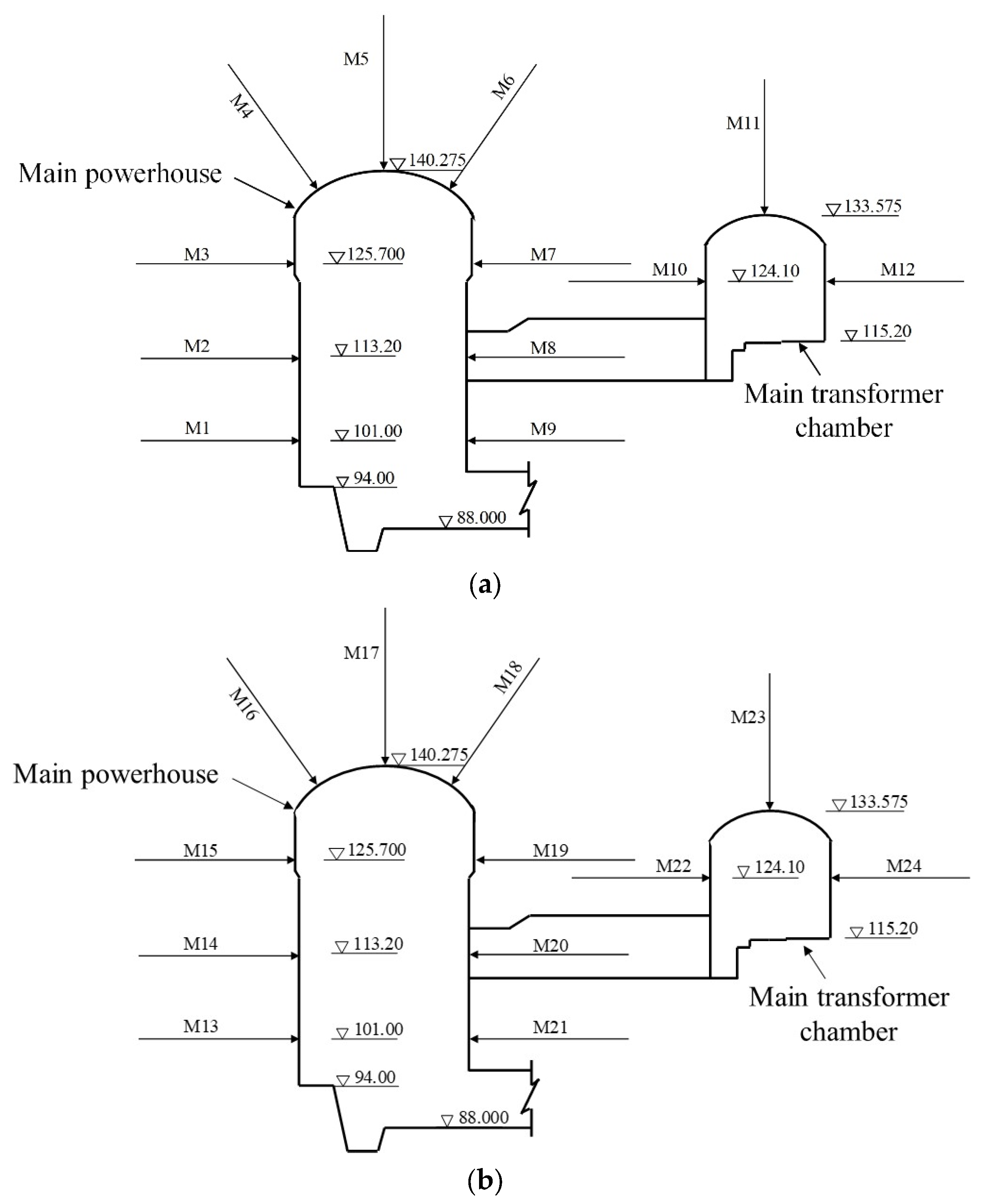
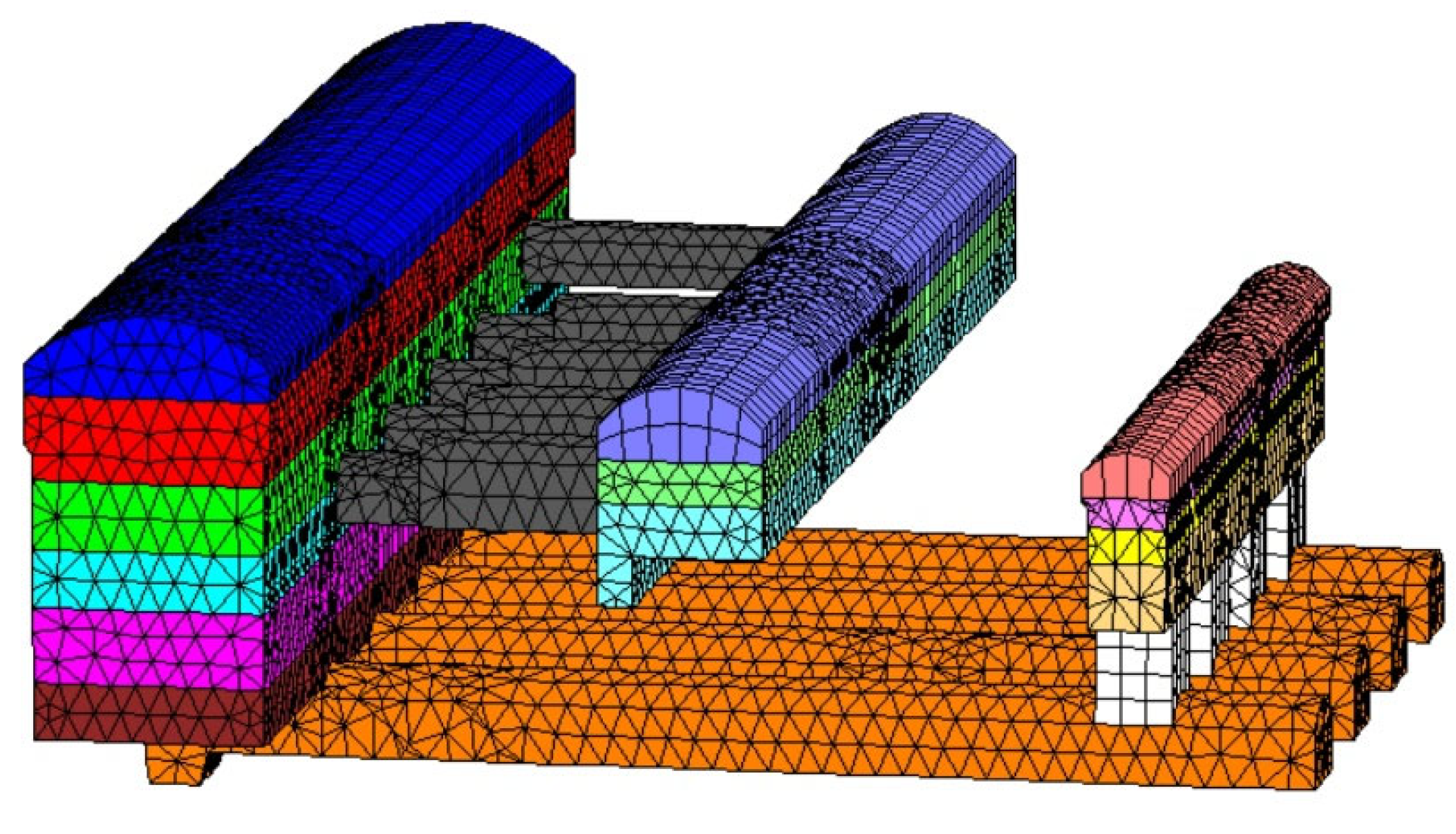
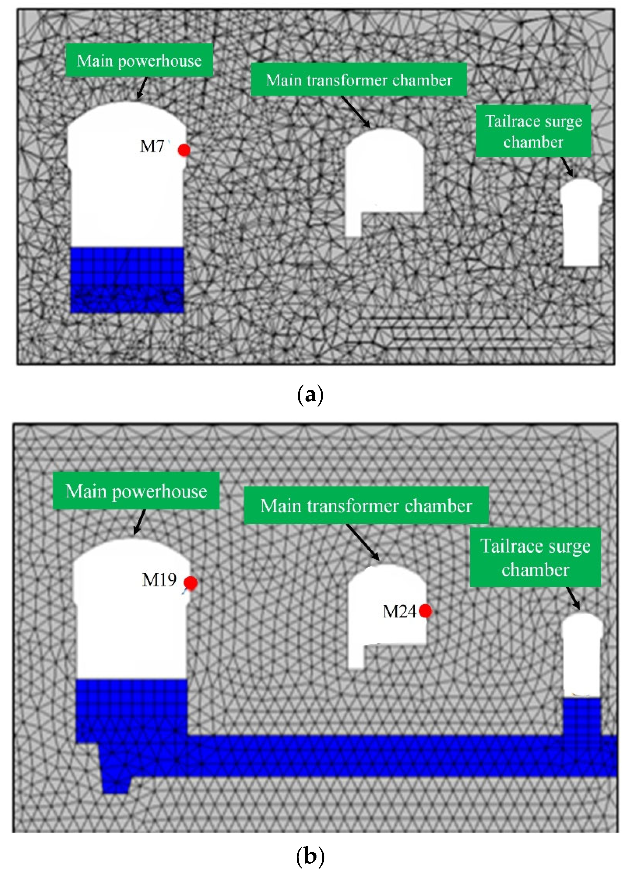
The Tai’an Pumped Storage Power Station in China is mainly composed of large caverns, including the main powerhouse, four omnibus bar caves, the main transformer chamber and a tailrace surge chamber. The surrounding rocks are mainly II and III granite, and there are four hydrogenerator sets arranged. The size of the main powerhouse is 180 m × 25.9 m × 53.675 m; the size of the main transformer chamber is 164 m × 17.5 m × 18.175 m; and the length of the omnibus bar cave is 35 m. Figure 11 shows the staged excavation. There are two displacement monitoring sections in the underground powerhouse. The layout of the corresponding monitoring points is shown in Figure 12. The FLAC3D calculation grid of the excavation body is shown in Figure 13, which includes 687,133 elements and 191,323 nodes, and the grid has been colored to distinguish the tunnel area and excavation sequence. The corresponding monitoring point layout is shown in Figure 14.
The measured displacements of monitoring points M7, M19 and M24 are selected to construct the objective function, as shown in Equation (14). The selected three measurement points are based on the three points of maximum deformation that have been recorded. The geomechanical parameters to be back-analysed are as follows: elastic modulus E1 of the surrounding rock upstream of the main powerhouse; elastic modulus E2 of the surrounding rock downstream of the #1 unit of the main powerhouse; elastic modulus E3 of the surrounding rock downstream of the main powerhouse units #2–4; elastic modulus E4 of the surrounding rock of the variable chamber; the cohesion c1 of the surrounding rock upstream of the main powerhouse; the cohesion c2 of the surrounding rock downstream of the main powerhouse and the internal friction angle φ. The parameter search intervals are set to 60 GPa ≤ E1 ≤ 80 GPa, 10 GPa ≤ E2 ≤ 30 GPa, 20 GPa ≤ E3 ≤ 40 GPa, 100 GPa ≤ E4 ≤ 300 GPa, 5 MPa ≤ c1 ≤ 7 MPa, 5 MPa ≤ c2 ≤ 7 MPa, and 40° ≤ φ ≤ 60°.
The GOA parameter is set to D = 7, N = 30, cmax = 1, and cmin = 1 × 10⁻⁵. The initial hyperparameters of the GPR model are set as lnl = [−1,−1,−1,−1,−1,−1,−1], lnσf = −1, σn = 1 × 10⁻⁶. Take the number of FLAC3D calls greater than or equal to 1000 as the convergence criterion.
The GOA-FLAC3D method and the method in this paper are used to invert the geomechanical parameters. The results are shown in Table 5 and Table 6. For the M7 and M19 monitoring points, the relative errors between the calculated and measured displacement values obtained by the GOA-GPR-FLAC3D method are only 1.44% and 2.65%, while the relative errors of the GOA-FLAC3D method are 7.81% and 15.72%. For monitoring point M24, the relative errors of the two methods are 0.06% and 0.73%, respectively, with little difference. Therefore, under the same condition that FLAC3D is called 1000 times, the optimization accuracy of the proposed method is significantly higher than that of GOA-FLAC3D, indicating the superiority of the proposed method.
7. Conclusions
To address the contradiction between obtaining the global optimal solution and the high calculation cost in the displacement back-analysis of underground engineering projects, a novel algorithm is proposed for the optimized back-analysis of geomechanical parameters. The main conclusions are as follows:
- (1)
- In this paper, a new intelligent optimization back-analysis algorithm was proposed, which provides a new tool for the rational determination of geomechanical parameters in underground engineering. The algorithm combines the low computational cost and strong fitting ability of the GPR surrogate model with the strong global optimization ability of the GOA. The test results of various benchmark functions showed that the algorithm can effectively guarantee the accuracy of the solution. The evaluation times of the GOA fitness function are greatly decreased, which improves the efficiency of the algorithm.
- (2)
- Because a large number of numerical calculations are required when applying the GOA to the back-analysis of geomechanical parameter optimization, resulting in low computational efficiency, a collaborative optimization back-analysis method called GOA-GPR-FLAC3D was proposed. The results of a case study and an engineering example showed that the proposed method has better performance in efficiency and accuracy, and is feasible for the high-dimensional, highly nonlinear back-analysis of geomechanical parameters in underground engineering.
In order to facilitate engineering applications, this paper only studies the measured displacement back-analysis method based on the classical Mohr–Coulomb constitutive model. In fact, the displacement back-analysis method is only one of the back-analysis methods, and parameters such as stress and strain can also be used as objects of the back-analysis method. In addition, in underground engineering, the deformation of surrounding rock is actually related to many factors, such as rock mass characteristics, support timing and support methods. Therefore, the acquisition of mechanical parameters of underground engineering rock mass for different back-analysis methods and different conditions should be discussed in further research.
Author Contributions
Conceptualization, J.L. and G.S.; methodology, W.S. and Y.Z.; software, W.S. and Y.Z.; validation, J.L., W.S. and G.S.; investigation, W.S.; data curation, W.S.; writing—original draft preparation, W.S.; writing—review and editing, J.L., W.S. and G.S.; visualization, W.S. and Y.Z.; project administration, J.L.; funding acquisition, G.S. All authors have read and agreed to the published version of the manuscript.
Funding
This research was funded by the National Natural Science Foundation of China for financial support (Grant Nos. 52169021 and 51869003), and the High-Level Innovation Team and Outstanding Scholar Program of Universities in Guangxi province. (Grant No. 202006).
Institutional Review Board Statement
Not applicable.
Informed Consent Statement
Not applicable.
Data Availability Statement
Not applicable.
Conflicts of Interest
The authors declare no conflict of interest.
References
- Jiang, Q.; Su, G.; Feng, X.; Chen, G.; Zhang, M.; Liu, C. Excavation optimization and stability analysis for large underground caverns under high geostress: A case study of the Chinese Laxiwa project. Rock Mech. Rock Eng. 2019, 52, 895–915. [Google Scholar] [CrossRef]
- Zhang, Y.; Su, G.; Liu, B.; Li, T. A novel displacement back analysis method considering the displacement loss for underground rock mass engineering. Tunn. Undergr. Space Technol. 2020, 95, 103141. [Google Scholar] [CrossRef]
- Sharifzadeh, M.; Tarifard, A.; Moridi, M.A. Time-dependent behavior of tunnel lining in weak rock mass based on displacement back analysis method. Tunn. Undergr. Space Technol. 2013, 38, 348–356. [Google Scholar] [CrossRef]
- Cai, M.; Morioka, H.; Kaiser, P.K.; Tasaka, Y.; Kurose, H.; Minami, M.; Maejima, T. Back-analysis of rock mass strength parameters using AE monitoring data. Int. J. Rock Mech. Min. 2007, 44, 538–549. [Google Scholar] [CrossRef]
- Feng, X.; Zhang, Z.; Sheng, Q. Estimating mechanical rock mass parameters relating to the Three Gorges Project permanent shiplock using an intelligent displacement back analysis method. Int. J. Rock Mech. Min. 2000, 37, 1039–1054. [Google Scholar] [CrossRef]
- Sakurai, S.; Takeuchi, K. Back Analysis of Measured Displacements of Tunnels. Rock Mech. Rock Eng. 1983, 3, 173–180. [Google Scholar] [CrossRef]
- Berti, M.; Bertello, L.; Bernardi, A.R.; Caputo, G. Back analysis of a large landslide in a flysch rock mass. Landslides 2017, 14, 2041–2058. [Google Scholar] [CrossRef]
- Oreste, P. Back-analysis techniques for the improvement of the understanding of rock in underground constructions. Tunn. Undergr. Space Technol. 2005, 20, 7–21. [Google Scholar] [CrossRef]
- Gioda, G. Indirect identification of the average elastic characteristics of rock masses. In Proceedings of the International Conference on Structural Foundations on Rock, Sydney, NSW, Australia, 7–9 May 1980; pp. 65–73. [Google Scholar]
- Asaoka, A.; Matsuo, M. An inverse problem approach to the predication of multidimensional consolidation behavior. Soil Found. 1984, 1, 95–108. [Google Scholar]
- Anandarajah, A.; Agarwal, D. Computer-aided calibration of a soil plasticity model. Int. J. Rock Mech. Min. 1991, 24, 85–97. [Google Scholar] [CrossRef]
- Khamesi, H.; Torabi, S.R.; Mirzaei-Nasirabad, H.; Ghadiri, Z. Improving the performance of intelligent back analysis for tunneling using optimized fuzzy systems: Case study of the Karaj subway line 2 in Iran. J. Comput. Civ. Eng. 2015, 29, 05014010. [Google Scholar] [CrossRef]
- Zhao, H.; Yin, S. Geomechanical parameters identification by particle swarm optimization and support vector machine. Appl. Math. Model. 2009, 33, 3997–4012. [Google Scholar] [CrossRef]
- Beiki, M.; Majdi, A.; Givshad, A.D. Application of genetic programming to predict the uniaxial compressive strength and elastic modulus of carbonate rocks. Int. J. Rock Mech. Min. 2013, 63, 159–169. [Google Scholar] [CrossRef]
- Levasseur, S.; Malecot, Y.; Boulon, M.; Flavigny, E. Statistical inverse analysis based on genetic algorithm and principal component analysis: Applications to excavation problems and pressuremeter tests. Int. J. Numer. Anal. Met. 2010, 34, 471–491. [Google Scholar] [CrossRef]
- Hashash, Y.M.A.; Levasseur, S.; Osouli, A.; Finno, R.; Malecot, Y. Comparison of two inverse analysis techniques for learning deep excavation response. Comput. Geotech. 2010, 37, 323–333. [Google Scholar] [CrossRef]
- Hajihassani, M.; Jahed Armaghani, D.; Kalatehjari, R. Applications of particle swarm optimization in geotechnical engineering: A comprehensive review. Geotech. Geol. Eng. 2018, 36, 705–722. [Google Scholar] [CrossRef]
- Knabe, T.; Schweiger, H.F.; Schanz, T. Calibration of constitutive parameters by inverse analysis for a geotechnical boundary problem. Can. Geotech. J. 2012, 49, 170–183. [Google Scholar] [CrossRef]
- Zhang, Y.; Chi, Z.; Sun, Y. A novel multi-class support vector machine based on fuzzy theories. In Proceedings of the International Conference on Intelligent Computing, Kunming, China, 16–19 August 2006; pp. 42–50. [Google Scholar]
- Lin, P.; Liu, X.; Chen, H.; Kim, J. Ant colony optimization analysis on overall stability of high arch dam basis of field monitoring. Sci. World J. 2014, 2014, 483243. [Google Scholar] [CrossRef]
- Zhang, Y.; Su, G.; Li, Y.; Wei, M.; Liu, B. Displacement back-Analysis of rock mass parameters for underground caverns using a novel intelligent optimization method. Int. J. Geomech. 2020, 20, 4020035. [Google Scholar] [CrossRef]
- Zhang, S.K.; Yin, S.D.; Wang, F.M.; Zhao, H.B. Characterization of in situ stress state and joint properties from extended leak-off tests in fractured reservoirs. Int. J. Geomech. 2017, 17, 1943–1954. [Google Scholar] [CrossRef]
- Ni, S.S.; Chi, S.C. Back analysis of permeability coefficient of high core rockfill dam based on particle swarm optimization and support vector machine. Chin. J. Geotech. Eng. 2017, 39, 727–734. [Google Scholar]
- Jiang, A.N. Optimization generator socket construction schemes of Shuibuya underground powerhouse based on intelligent back analysis. Chin. J. Rock Mech. Eng. 2008, 29, 1372–1376. [Google Scholar]
- Saremi, S.; Mirjalili, S.; Lewis, A. Grasshopper optimisation algorithm: Theory and application. Adv. Eng. Softw. 2017, 105, 30–47. [Google Scholar] [CrossRef] [Green Version]
- Akash, S. A comprehensive study of chaos embedded bridging mechanisms and crossover operators for grasshopper optimisation algorithm. Expert Syst. Appl. 2019, 132, 166–188. [Google Scholar]
- Hoffer, J.G.; Geiger, B.C.; Kern, R. Gaussian process surrogates for modeling uncertainties in a use case of forging superalloys. Appl. Sci. 2022, 12, 1089. [Google Scholar] [CrossRef]
- Aigrain, S.; Parviainen, H.; Pope, B.J.S. K2SC: Flexible systematics correction and detrending of K2 light curves using Gaussian process regression. Mon. Not. R. Astron. Soc. 2016, w706, 2408–2419. [Google Scholar] [CrossRef] [Green Version]
- Lee, D.; Park, H.; Yoo, C.D. Face alignment using cascade Gaussian process regression trees. In Proceedings of the IEEE Conference on Computer Vision and Pattern Recognition, Boston, MA, USA, 7–12 June 2015; pp. 4204–4212. [Google Scholar]
- Rasmussen, C.E. Gaussian processes in machine learning. In Summer School on Machine Learning; Springer: Berlin, Germany, 2003; pp. 63–71. [Google Scholar]
- Braja, M. Advanced Soil Mechanics, 4th ed.; Taylor & Francis: Boca Raton, FL, USA, 2014; pp. 403–405. [Google Scholar]
- Verónica, M.; Eduardo, B.; Alexandra, O. Implementation of a model of elastoviscoplastic consolidation behavior in Flac 3D. Comput. Geotech. 2018, 98, 132–143. [Google Scholar]
- Mina, D.; Forcellini, D. Soil–structure interaction assessment of the 23 November 1980 Irpinia-Basilicata earthquake. Geosciences 2020, 10, 152. [Google Scholar] [CrossRef] [Green Version]
- Karapetrou, S.; Fotopoulou, S.; Pitilakis, K. Seismic vulnerability assessment of high-rise non-ductile RC buildings considering soil–structure interaction effects. Soil Dyn. Earthq. Eng. 2015, 73, 42–57. [Google Scholar] [CrossRef]
- Li, Y.; Guo, Y.; Zhu, W.; Li, S.; Zhou, H. A modified initial in-situ stress inversion method based on FLAC3D with an engineering application. Open Geosci. 2015, 7, 824–835. [Google Scholar] [CrossRef]
- Forcellini, D. Assessment on geotechnical seismic isolation (GSI) on bridge configurations. Innov. Infrastruct. Solut. 2017, 2, 9. [Google Scholar] [CrossRef]
- Forcellini, D. Soil-structure interaction analyses of shallow-founded structures on a potential-liquefiable soil deposit. Soil. Dyn. Earthq. Eng. 2020, 133, 106108. [Google Scholar] [CrossRef]
Figure 1.
Schematic of the interaction between individual grasshoppers.

Figure 2.
Schematic of the empirical dataset for the surrogate model.

Figure 3.
Flowchart of the GOA-GPR optimization algorithm.

Figure 4.
Three-dimensional space surface diagram of Case 1.

Figure 5.
Convergence curve of the test function in Case 1.

Figure 6.
Three-dimensional space surface diagram of Case 2.

Figure 7.
Convergence curve of the test function in Case 2.

Figure 8.
Flowchart of the GOA-GPR-FLAC3D method.

Figure 9.
Computational grid of FLAC3D.

Figure 10.
Layout of monitoring points.

Figure 11.
Schematic diagram of excavation by stages of the powerhouse (unit: m).

Figure 12.
The layout map of the displacement monitoring points section. (a) The monitoring points at the 0 + 15 m section to the left of the powerhouse. (b) The monitoring points at the 0 + 54 m section to the left of the powerhouse.
Figure 12.
The layout map of the displacement monitoring points section. (a) The monitoring points at the 0 + 15 m section to the left of the powerhouse. (b) The monitoring points at the 0 + 54 m section to the left of the powerhouse.

Figure 13.
The computing grid of excavated rock.

Figure 14.
The location map of selected monitoring points in the FLAC3D model. (a) The monitoring point at the 0 + 15 m section to the left of the powerhouse. (b) The monitoring point at the 0 + 54 m section to the left of the powerhouse.
Figure 14.
The location map of selected monitoring points in the FLAC3D model. (a) The monitoring point at the 0 + 15 m section to the left of the powerhouse. (b) The monitoring point at the 0 + 54 m section to the left of the powerhouse.


Table 1.
Comparison of calculation results for Case 1.
| Method | GOA | GOA-GPR |
|---|---|---|
| The optimal value/10−6 | 9.18 | 9.73 |
| The worst value/10−6 | 9.51 | 9.94 |
| Average number of function evaluations | 369,600 | 37,612 |
Table 2.
Comparison of calculation results for Case 2.
| Method | GOA | GOA-GPR |
|---|---|---|
| The optimal value/10−4 | 9.18 | 9.73 |
| The worst value/10−4 | 9.51 | 9.94 |
| Average number of function evaluations | 369,600 | 37,612 |
Table 3.
The measured displacements of points.
| Direction | Displacement Value of Each Monitoring Point (mm) | ||||
|---|---|---|---|---|---|
| 1 | 2 | 3 | 4 | 5 | |
| Horizontal direction () | −27.0159 | −23.3271 | −19.6929 | −14.6111 | 0 |
| Vertical direction () | 0 | −14.5982 | −19.6261 | −23.2481 | −26.8916 |
Table 4.
The results calculated by the two methods.
| Methods | GOA-FLAC3D | GOA-GPR-FLAC3D | ||||
|---|---|---|---|---|---|---|
| Parameter | E/GPa | c/MPa | φ/° | E/GPa | c/MPa | φ/° |
| Real solution | 2.2 | 1.1 | 30 | 2.2 | 1.1 | 30 |
| Back-analysis result | 2.279 | 1.160 | 29.8 | 2.195 | 1.125 | 30.3 |
| Relative error/% | 3.59 | 5.46 | 0.67 | 0.23 | 2.27 | 1.00 |
| Fitness | 0.0426 | 0.0362 | ||||
| Fitness function evaluation times | 9254 | 1077 | ||||
| Computing time/s | 1.73 × 10⁵ | 2.26 × 10³ | ||||
Table 5.
Back-analysis results of geomechanical parameters by two methods.
| Method | Geomechanical Parameters | ||||||
|---|---|---|---|---|---|---|---|
| E1/GPa | E2/GPa | E3/GPa | E4/GPa | c1/MPa | c2/MPa | φ/° | |
| GOA-FLAC3D | 65.21 | 21.67 | 28.94 | 215.10 | 6.74 | 6.85 | 56.20 |
| GOA-GPR-FLAC3D | 65.28 | 21.61 | 28.91 | 215.13 | 6.70 | 6.79 | 56.16 |
Table 6.
Comparison of displacements obtained from calculation and measurement.
| Monitoring Point | Measured Displacement/mm | GOA-FLAC3D | GOA-GPR-FLAC3D | ||
|---|---|---|---|---|---|
| Calculated Displacement/mm | Related Error/% | Calculated Displacement/mm | Related Error/% | ||
| M7 | 5.833 | 5.377 | 7.81 | 5.749 | 1.44 |
| M19 | 4.044 | 4.680 | 15.72 | 4.151 | 2.65 |
| M24 | 1.633 | 1.645 | 0.73 | 1.632 | 0.06 |
Publisher’s Note: MDPI stays neutral with regard to jurisdictional claims in published maps and institutional affiliations. |
© 2022 by the authors. Licensee MDPI, Basel, Switzerland. This article is an open access article distributed under the terms and conditions of the Creative Commons Attribution (CC BY) license (https://creativecommons.org/licenses/by/4.0/).
Share and Cite
MDPI and ACS Style
Li, J.; Sun, W.; Su, G.; Zhang, Y. An Intelligent Optimization Back-Analysis Method for Geomechanical Parameters in Underground Engineering. Appl. Sci. 2022, 12, 5761. https://0-doi-org.brum.beds.ac.uk/10.3390/app12115761
AMA Style
Li J, Sun W, Su G, Zhang Y. An Intelligent Optimization Back-Analysis Method for Geomechanical Parameters in Underground Engineering. Applied Sciences. 2022; 12(11):5761. https://0-doi-org.brum.beds.ac.uk/10.3390/app12115761
Chicago/Turabian StyleLi, Jianhe, Weizhe Sun, Guoshao Su, and Yan Zhang. 2022. "An Intelligent Optimization Back-Analysis Method for Geomechanical Parameters in Underground Engineering" Applied Sciences 12, no. 11: 5761. https://0-doi-org.brum.beds.ac.uk/10.3390/app12115761
Note that from the first issue of 2016, this journal uses article numbers instead of page numbers. See further details here.