Computational Algorithms Underlying the Time-Based Detection of Sudden Cardiac Arrest via Electrocardiographic Markers

Featured Application

This study explores the potential use of supervised machine learning for the early detection of sudden cardiac arrest using electrocardiographic markers, such as heart rate, R-R interval duration, and heart rate variability.

Abstract

Early detection of sudden cardiac arrest (SCA) is critical to prevent serious repercussion such as irreversible neurological damage and death. Currently, the most effective method involves analyzing electrocardiogram (ECG) features obtained during ventricular fibrillation. In this study, data from 10 normal patients and 10 SCA patients obtained from Physiobank were used to statistically compare features, such as heart rate, R-R interval duration, and heart rate variability (HRV) features from which the HRV features were then selected for classification via linear discriminant analysis (LDA) and linear and fine Gaussian support vector machines (SVM) in order to determine the ideal time-frame in which SCA can be accurately detected. The best accuracy was obtained at 2 and 8 min prior to SCA onset across all three classifiers. However, accuracy rates of 75–80% were also obtained at time-frames as early as 50 and 40 min prior to SCA onset. These results are clinically important in the field of SCA, as early detection improves overall patient survival.

1. Introduction

Sudden cardiac arrest (SCA) is the sudden unexpected loss of heart function less than 1 h from the onset of symptoms [1,2]. SCA arises when a triggering factor that is either acquired or genetically-determined affects an anatomical or physiological substrate, manifesting into an abnormal heart rhythm such as ventricular tachycardia, which ultimately degenerates into the fatal ventricular fibrillation (VF) rhythm [3].

SCA can occur at any age in a patient with or without a detectable heart disease [4]. Approximately 15,000 Australians per year experience SCA and only 6–13% of patients survive more than one year after the event [5]. SCA is one of the major causes of cardiovascular mortality and is a major public health issue both nationally and globally, with the annual cost of SCA amounting to approximately $33 billion USD [6]. This economic and health burden of SCA poses to society can be reduced with the improvement of patient outcomes through better detection systems [7].

However, the main challenge associated with SCA detection lies in the fact that SCA can manifest in the complete absence of symptoms. Various methods have been investigated for the detection of SCA, each demonstrating strengths in various patient populations. Cardiac imaging modalities such as cardiac magnetic resonance imaging, echocardiography and cardiac positron emission tomography were found to be useful in patients with a suspected structural heart disease [8]. However, there are many cases in which SCA may arise as a result of a non-cardiac cause. Electrophysiology study had also been investigated as a potential detection method, however, there is limited data on its prognostic value for SCA and it is limited due to its poor negative predictive value and its decrease in sensitivity with polymorphic ventricular tachycardia rhythms [9]. The current most commonly explored detection method for SCA is electrocardiography (ECG). Early studies had already established the clinical importance of ECG detection, as 95% of SCA patients were found to have abnormal ECG readings [10]. These early studies have highlighted the usefulness of ECG monitoring for SCA detection as it can aid in understanding the changes preceding the VF rhythm and have identified potential markers that may trigger SCA. The ECG markers that have been currently explored include: QTc interval, QRS duration, R-R interval, ST segment elevation, T-wave amplitude, and T-peak-to-T-end [11,12,13,14]. Though its efficacy as a detection method has been well established, the field is still developing and future large cohort studies on specific patient populations still need to be conducted. Overall, although a majority of both invasive and non-invasive tests have been employed and evaluated, there is currently no optimal detection method nor criteria specific for SCA [15].

Currently, computer algorithms have been developed and utilized in the clinical setting for the quick detection of critical events such as ventricular fibrillation, in the case of SCA. These pattern recognition methods aim to either assign an individual heartbeat to a specific class or to detect the underlying pathology using information obtained from measurable features of the ECG, such as the R-R interval duration. The assumption is that features of individuals in the same class have similar values and, thus, occupy a specific region in the multidimensional feature space separated from other classes [16]. Early studies on pattern recognition algorithms utilized linear classification methods, such as linear discriminant analysis, which assumed that biological signals were linear in nature. Although these methods provided reasonable results, the underlying non-linear features of these signals were ignored. As a majority of biological signals are non-linear in nature, this led to the need for further classification and, thus, research interest had shifted to non-linear classification methods, such as support vector machines [17]. However, limitations lie in the current literature as time-frames of only up to 5 min prior to the onset of SCA have been thoroughly investigated, which, when applied to the clinical setting, does not provide enough time for a patient to respond with sufficient time to reach the hospital. The overall survival rate decreases by 10% each minute the patient remains in VF, thus, high importance is placed on detection as early identification and management is critical.

Since the early detection of SCA is highly important yet not well established, the aim of this study is to, first, statistically compare the importance of various ECG features, such as heart rate and R-R interval related markers, between normal and patients at risk of SCA and, secondly, and most importantly, to determine the ideal time-frame spanning up to three hours prior to the onset of VF in which electrocardiographic changes alluding to SCA can be detected and accurately classified.

2. Materials and Methods

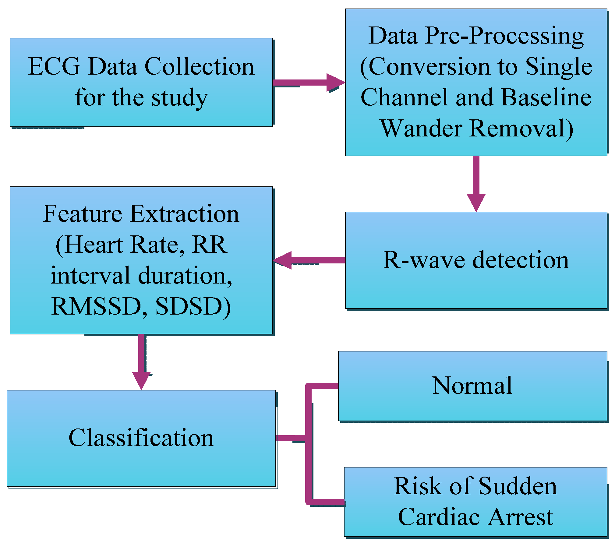
Two databases from the physiological signal online archive Physiobank were utilized in this study: the Sudden Cardiac Death Holter Database (SDDB) and the MIH-BIH Normal Sinus Rhythm Database (NSRDB). The normal patient cohort consisted of 10 records selected from the NSRDB (four males, aged 32 to 45 and six females, aged 35 to 50). The SCA cohort consisted of 10 records selected from the SDDB (five males, aged 34 to 74, four females, aged 62 to 82, and one patient of unknown gender, aged 62). Each ECG dataset consisted of 24-h Holter ECG recordings before and after the SCA event [18]. The full methodology of this study has been outlined in Figure 1 below.

2.1. Data Preprocessing

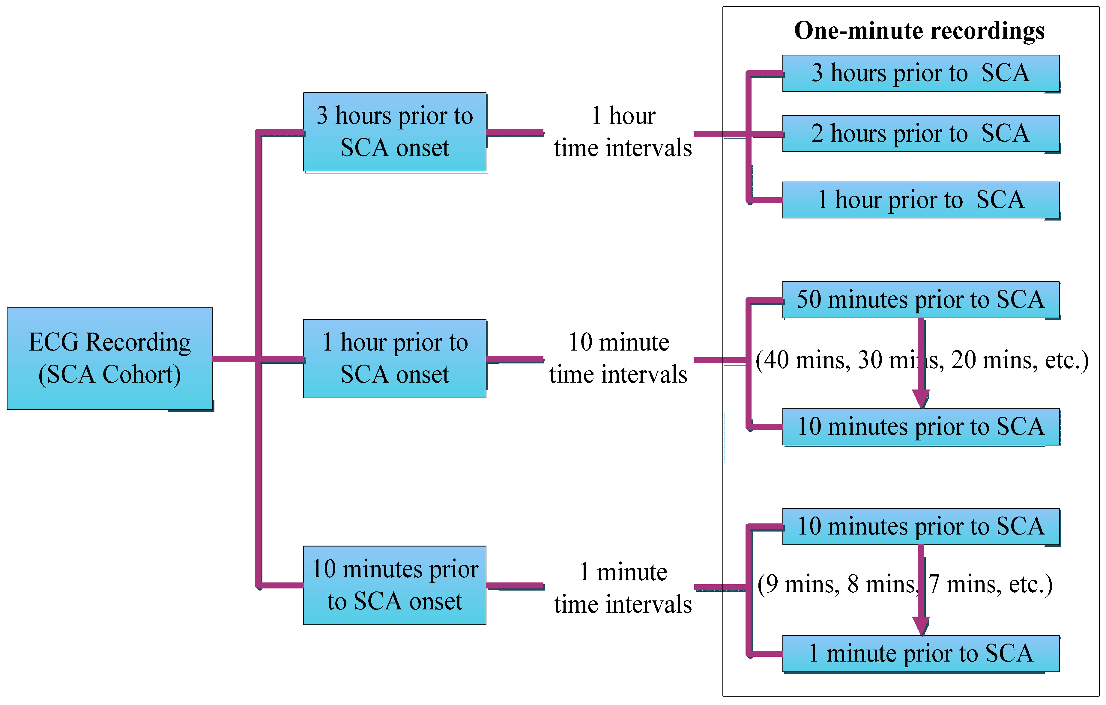
Each dataset in the SCA cohort was first segmented into one-minute intervals every hour, three hours prior to the onset of the SCA event (3 h, 2 h, and 1 h), then partitioned into one-minute intervals every 10 min prior to SCA onset (50 min, 40 min, etc.) and from 10 min into one-minute intervals every minute until the onset of SCA (10 min, 9 min, etc.). For the normal cohort, five random one-minute intervals were selected from the fourth hour of recording and isolated (See Figure 2 below).

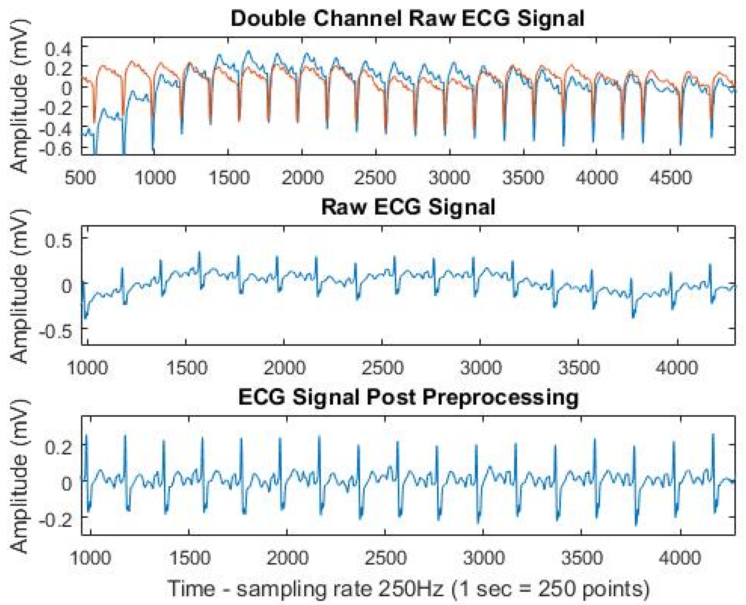
Both the normal and SCA cohort datasets were then converted from a double-channel ECG recording to a single-channel recording (see Figure 3). All ECG recordings were then subjected to baseline wander removal; a Butterworth band-pass filter with cutoff frequencies between 0.5 Hz and 45 Hz was applied to remove both baseline drift and high-frequency noise. The filtered ECG was then used in all subsequent steps with a sampling rate of 250 Hz (see Figure 3). All data preprocessing steps were conducted in MATLAB R2016a.

2.2. ECG Feature Extraction

Following preprocessing the R wave of the filtered ECG signal was then detected using MATLAB for feature extraction. As the ECG signals utilized in this study did not consistently exhibit the normal ECG waveform even after signal preprocessing (either due to the underlying condition of the patient or due to external noise interference), there was difficulty in detecting and extracting features pertaining to the P, Q, R, S, and T waves. Since the R wave was easily detectable, a set of time-domain-related R-wave features were selected. The following features were then extracted and analyzed: (1) the mean resting heart rate (beats per minute); and (2) the mean R-R interval duration (ms), the duration between two successive R waves [19]:

$$R{R}_{mean}=\frac{1}{N}{{\displaystyle \sum }}^{\text{}}RR\left(i\right)$$

(1)

Two measures of heart rate variability (HRV): (3) RMSSD (ms), the square root of the mean of differences between all adjacent R-R intervals:

$$RMSSD=\sqrt{\frac{1}{N}{{\displaystyle \sum }}^{\text{}}{(RR\left(i+1\right)-RR\left(i\right))}^2}$$

(2)

and (4) SDSD (ms), the standard deviation of differences between all adjacent R-R intervals:

$$SDSD=\sqrt{\frac{1}{N}{\displaystyle \sum }_{i=1}^n{(R{R}_{\left(diff\right)}-{\overline{RR}}_{\left(diff\right)})}^2}$$

(3)

A one-way analysis of variance (ANOVA) with repeated measures was then conducted to determine if there were statistically significant differences between the normal and SCA cohort for each feature, as well as differences between each time interval prior to, and during, the onset of SCA. The statistical significance used in this study was 0.05 (95% confidence interval). Post-hoc analysis was performed using Tukey’s honest significant difference (HSD) test in instances where statistical significance has been reached.

2.3. Classification and Machine Learning

Once all data had been imported into MATLAB for classification, all three R-R-related SCA features (mean R-R interval duration, RMSSD and SDSD) were then compiled into a singular 1200 × 3 matrix based on the time window (e.g., “3 h prior to SCA”). The data was then subjected to statistical classification via various classifiers using the Classification Learner App in MATLAB, in order to discriminate between the features extracted from a normal patient to that of a patient at risk of SCA. Each classifier generates a pattern recognition model based on a given set in order to classify future input datasets for SCA risk detection [20]. The data was first subjected to linear discriminant analysis via a linear classifier, which aims to separate input vectors into classes through the use of linear decision boundaries. The within-class scatter matrix (S_w) is modelled as:

$$S_w={\displaystyle \sum }_{i=1}^C{\displaystyle \sum }_{x\in C_i}\left(x-m_i\right){\left(x-m_i\right)}^t$$

(4)

where C denotes the number of classes, C_i is the set of data belonging to a class and m_i denotes the mean of the class. The between-class scatter matrix (S_B) is modelled as:

$$S_B={\displaystyle \sum }_{i=1}^C\left(m_i-m\right){\left(m_i-m\right)}^t$$

(5)

where m denotes the mean of all classes. The criterion function is defined as:

$$J\left(W\right)=\frac{\left|W^t{S}_{B}W\right|}{W^t{S}_{w}W}$$

(6)

The overall result is a transformation matrix that maximizes the ratio of between class variance to within class variance so that adequate class separability is obtained [20].

Linear classification was then followed by binary support vector machine (SVM) classification with both a linear SVM and a non-linear fine Gaussian SVM. A support vector machine creates a decision surface by constructing an optimal hyperplane which separates two classes which, in this case, are normal patients and patients at risk of SCA. The optimum hyperplane is found by maximizing the distance between two hyperplanes: w∙x + b = +1 and w∙x + b = −1 which is 2/‖w‖. A slack variable ξ_i is then introduced and the optimal hyperplane is then determined by minimizing:

$$C{\displaystyle \sum }_{i=1}^k\xi i+\frac{1}{2}\Vert w{\Vert }^2$$

(7)

where C denotes a cost-constant involving margin size and error. The Langrange multiplier α_i is then used to find the optimal hyperplane by maximizing:

$$L\left(\alpha \right)={\displaystyle \sum }_{i=1}^n{\alpha }_i-\frac{1}{2}{\displaystyle \sum }_{i=1}^n{\displaystyle \sum }_{j=1}^n{\alpha }_i{\alpha }_j{z}_i{z}_j\left(x_{\mathrm{i}}·x_j\right)$$

(8)

As the data in this study is non-linear, it can be linearly classified using the RBF function [21]:

$$k\left(x_i,x_j\right)=\exp (-\gamma \Vert x_i-x_j{\Vert }^2)$$

(9)

Performance measurement was then conducted using the performance indicators, accuracy, sensitivity and specificity which were calculated via the confusion matrix generated by MATLAB [19]:

The accuracy for each time-frame and each classification method were obtained and recorded in order to determine the earliest time-frame in which SCA can be accurately detected. All classifiers were subjected to five-fold cross-validation. The most accurate time-frame and the earliest time-frame exhibiting reasonable accuracy (relative to the values obtained in the preceding time intervals) across all classifiers were then isolated and subjected to further testing to evaluate the sensitivity and specificity across the three different classification methods.

Sensitivity or True Positive Rate (%), the ability of the classifier to correctly identify a sudden cardiac arrest patient is calculated as follows:

$$Sensitivity=\frac{TP}{\left(TP+FN\right)}\times 100$$

(10)

Specificity (%), the ability of the classifier to correctly identify a normal patient is calculated as follows:

$$Specificity=\frac{TN}{\left(TN+FP\right)}\times 100$$

(11)

where true positive (TP) indicates the number of data inputs that are correctly identified as SCA patients. False positive (FP) denotes the number of data inputs that identify normal patient as at risk of SCA. True negative (TN) is the number of data inputs that are correctly identified as normal patients. False negative (FN) indicates the number of data inputs that identify SCA patients as normal patients.

3. Results

3.1. Feature Selection

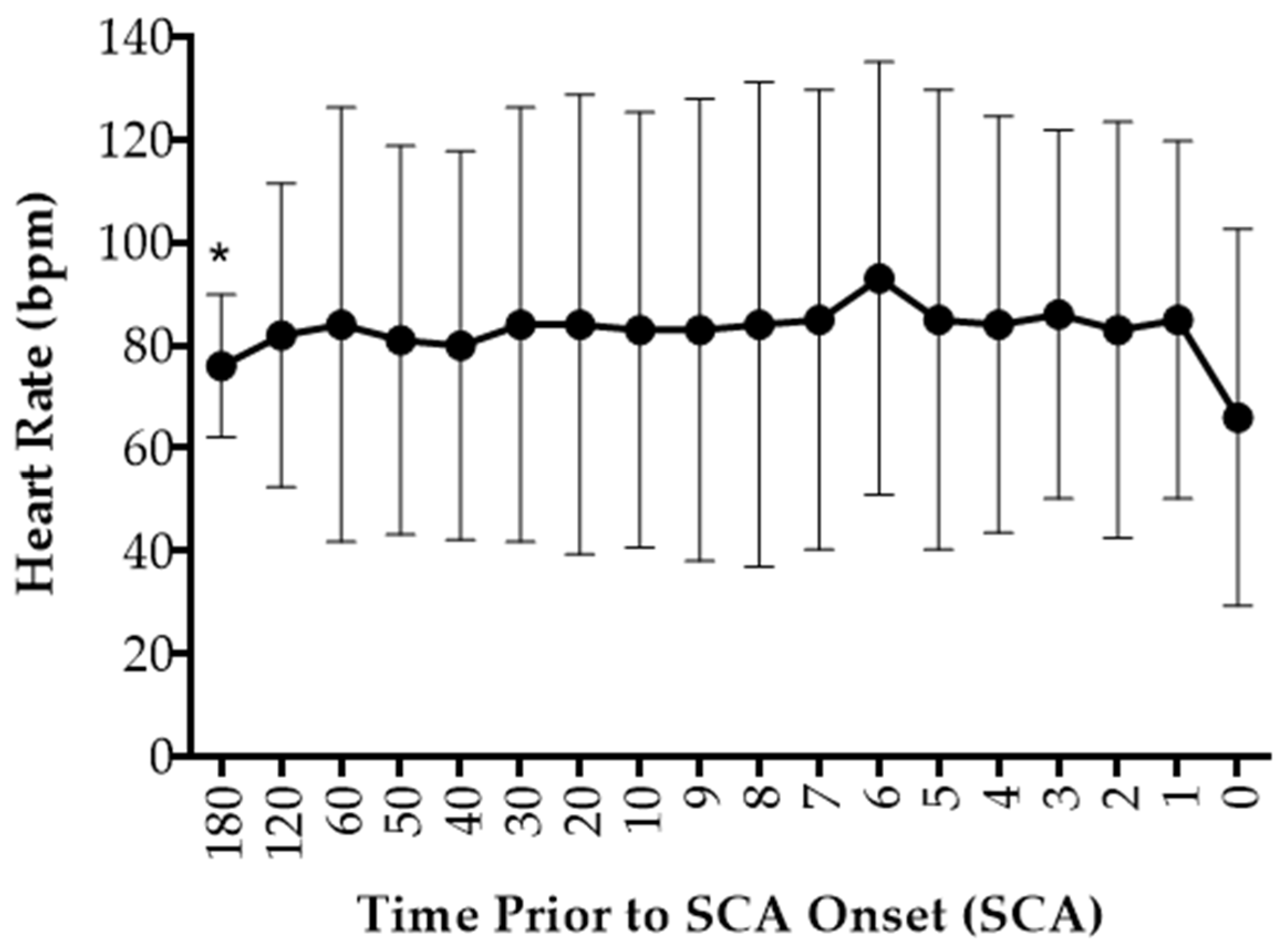
During SCA, the mean resting heart rate was observed to continuously fluctuate from 3 h prior to the onset of SCA to 1 min before the onset of SCA. However, a sudden decrease in heart rate between 1 min prior to SCA and during the onset of SCA was observed (See Figure 4). Compared to the normal patients, SCA patients exhibited a higher mean resting heart rate, with an 18.7 ± 3.5 bpm difference observed between the two cohorts (See

Table A1. Tabular summary of the extracted ECG features: mean resting heart rate, mean R-R interval duration, and heart rate variability features (RMSSD and SDSD) (n = 20).

	Heart Rate (bpm)	R-R Interval Duration (ms)	RMSSD 1 (ms)	SDSD 2 (ms)
Normal (n = 10)	65 ± 5.2	697 ± 60	52 ± 5.00	43 ± 5.00
SCA (n = 10)
3 h prior	76 ± 13.9	809 ± 134	43 ± 4.00	33 ± 4.00
2 h prior	82 ± 29.6	823 ± 141	56 ± 4.00	38 ± 5.0
1 h prior	84 ± 29.6	830 ± 153	97 ± 12.0	58 ± 6.0
50 min prior	81 ± 42.3	841 ± 144	124 ± 11.0	86 ± 7.0
40 min prior	80 ± 37.8	862 ± 150	83 ± 9.00	59 ± 7.0
30 min prior	84 ± 42.5	850 ± 154	99 ± 9.00	67 ± 7.0
20 min prior	84 ± 44.7	844 ± 175	74 ± 6.00	63 ± 4.0
10 min prior	83 ± 42.4	845 ± 166	98 ± 12.0	65 ± 8.0
9 min prior	83 ± 44.9	847 ± 172	73 ± 7.00	55 ± 5.00
8 min prior	84 ± 47.2	814 ± 148	84 ± 8.00	56 ± 5.00
7 min prior	85 ± 44.7	809 ± 167	74 ± 7.00	51 ± 4.00
6 min prior	93 ± 42.2	805 ± 170	81 ± 5.00	49 ± 4.00
5 min prior	85 ± 44.7	798 ± 167	71 ± 7.00	65 ± 4.00
4 min prior	84 ± 40.5	797 ± 184	104 ± 7.00	86 ± 7.00
3 min prior	86 ± 35.8	794 ± 212	110 ± 10.0	94 ± 6.00
2 min prior	83 ± 40.5	817 ± 185	102 ± 10.0	66 ± 5.00
1 min prior	85 ± 34.8	813 ± 163	118 ± 11.0	92 ± 7.00
Onset of SCA	66 ± 36.7	5827 ± 9.846	317 ± 240.6	258 ± 231.5

¹ RMSSD: the square root of the mean of differences between adjacent R-R intervals; ² SDSD: the standard deviation of differences between adjacent R-R intervals.

, Appendix A). Overall there was no statistically significant difference in mean resting heart rate between normal and SCA patients with the exemption of 3 h prior to SCA, F(1,18) = 4.70, p = 0.04 and 6 min prior to SCA, F(1,18) = 4.23, p = 0.05 (See

Table A2. Tabular summary of the repeated measures ANOVA conducted on the ECG features extracted from the normal patient cohort vs. SCA patient cohort (n = 20).

	Heart Rate (bpm)		RR Interval Duration (ms)		RMSSD (ms)		SDSD (ms)
Time Frame	F(1,18)	p-value	F(1,18)	p-value	F(1,18)	p-value	F(1,18)	p-value
3 h prior	4.70	0.04	4.57	0.05 *	0.17	0.68	0.21	0.65
2 h prior	3.72	0.07	2.71	0.03 *	0.01	0.90	0.03	0.86
1 h prior	2.39	0.14	5.34	0.03 *	1.22	0.28	0.40	0.54
50 min prior	2.24	0.15	6.88	0.02 *	3.31	0.09	2.35	0.14
40 min prior	1.72	0.20	8.50	0.01 **	0.93	0.35	0.38	0.55
30 min prior	2.06	0.17	7.09	0.02 *	2.07	0.17	0.94	0.35
20 min prior	2.41	0.14	5.41	0.03 *	0.77	0.39	0.93	0.35
10 min prior	1.92	0.18	5.89	0.03 *	1.19	0.29	0.63	0.44
9 min prior	1.82	0.19	5.79	0.03 *	0.63	0.44	0.57	0.33
8 min prior	2.25	0.15	4.36	0.05	1.20	0.29	0.32	0.58
7 min prior	2.79	0.11	3.32	0.08	0.69	0.42	0.16	0.69
6 min prior	4.23	0.05 *	3.00	0.10	1.62	0.22	0.09	0.76
5 min prior	3.03	0.10	2.71	0.12	0.78	0.39	1.15	0.30
4 min prior	3.27	0.09	2.32	0.15	3.24	0.09	2.74	0.12
3 min prior	3.04	0.10	1.72	0.21	4.28	0.05 *	4.14	0.06
2 min prior	1.68	0.21	3.28	0.09	2.04	0.17	1.01	0.33
1 min prior	1.79	0.20	3.74	0.07	2.95	0.10	3.04	0.10
Onset of SCA	0.02	0.88	2.71	0.12	1.92	0.18	2.61	0.12

, Appendix B). Post-hoc analyses using Tukey Honestly Significant Difference (Tukey HSD) indicated that there was a significant difference in mean resting heart rate observed between both patient cohorts at 3 h prior to SCA (p = 0.04), but however found no significant difference in mean resting heart rate observed between the two patient cohorts at 6 min prior to SCA onset (p = 0.06) (See

Table A4. Tabular summary of post-hoc Tukey’s HSD conducted on ECG feature extracted from the normal patient cohort vs. the SCA patient cohort at time-frames which have reached statistical significance (n = 20).

ECG Feature	Time-frame	Tukey’s HSD	Tukey’s HSD	Tukey’s HSD
		Q Statistic	p-Value	Inference
Heart Rate	3 h prior	3.07	0.04	* p < 0.05 1
	6 min prior	2.91	0.05	Insignificant
R-R Interval Duration	3 h prior	3.02	0.05	* p < 0.05
	2 h prior	3.30	0.03	* p < 0.05
	1 h prior	3.27	0.03	* p < 0.05
	50 min prior	3.71	0.02	* p < 0.05
	40 min prior	4.12	0.009	** p < 0.01 2
	30 min prior	3.77	0.02	* p < 0.05
	20 min prior	3.29	0.03	* p < 0.05
	10 min prior	3.43	0.03	* p < 0.05
	9 min prior	2.41	0.03	* p < 0.05
RMSSD	3 min prior	2.93	0.05	Insignificant

Asterisks denote statistical significance by Tukey’s HSD where ¹ *p < 0.05 and ² ** p < 0.01.

, Appendix B). Similarly, there was no statistically significant difference in heart rate between each time-frame and the onset of SCA (See

Table A3. Tabular summary of the repeated measures ANOVA conducted on the ECG features obtained from time-frames prior to SCA vs. during the onset of SCA (n = 10).

	Heart Rate (bpm)		RR Interval Duration (ms)		RMSSD (ms)		SDSD (ms)
Time Frame	F(1,18)	p-value	F(1,18)	p-value	F(1,18)	p-value	F(1,18)	p-value
3 h vs. Onset	0.64	0.43	2.60	0.13	1.93	0.18	2.61	0.12
2 h vs. Onset	1.33	0.26	2.58	0.13	1.93	0.18	2.61	0.12
1 h vs. Onset	1.19	0.29	2.58	0.13	1.92	0.18	2.60	0.12
50 min vs. Onset	1.00	0.33	2.56	0.13	1.92	0.18	2.60	0.12
40 min vs. Onset	0.86	0.37	2.55	0.13	1.93	0.18	2.60	0.12
30 min vs. Onset	1.07	0.32	2.55	0.13	1.92	0.18	2.60	0.12
20 min vs. Onset	1.21	0.29	2.56	0.13	1.92	0.18	2.60	0.12
10 min vs. Onset	0.99	0.33	2.56	0.13	1.92	0.18	2.60	0.12
9 min vs. Onset	0.98	0.34	2.56	0.13	1.93	0.18	2.60	0.12
8 min vs. Onset	1.14	0.30	2.59	0.12	1.93	0.18	2.60	0.12
7 min vs. Onset	1.14	0.25	2.59	0.12	1.93	0.18	2.61	0.12
6 min vs. Onset	2.31	0.15	2.60	0.12	1.93	0.18	2.61	0.12
5 min vs. Onset	1.49	0.24	2.60	0.12	1.93	0.18	2.60	0.12
4 min vs. Onset	1.43	0.25	2.61	0.12	1.92	0.18	2.60	0.12
3 min vs. Onset	1.49	0.24	2.61	0.12	1.92	0.18	2.60	0.12
2 min vs. Onset	0.83	0.38	2.59	0.13	1.92	0.18	2.60	0.12
1 min vs. Onset	1.00	0.33	2.59	0.12	1.93	0.18	2.60	0.12

, Appendix B).

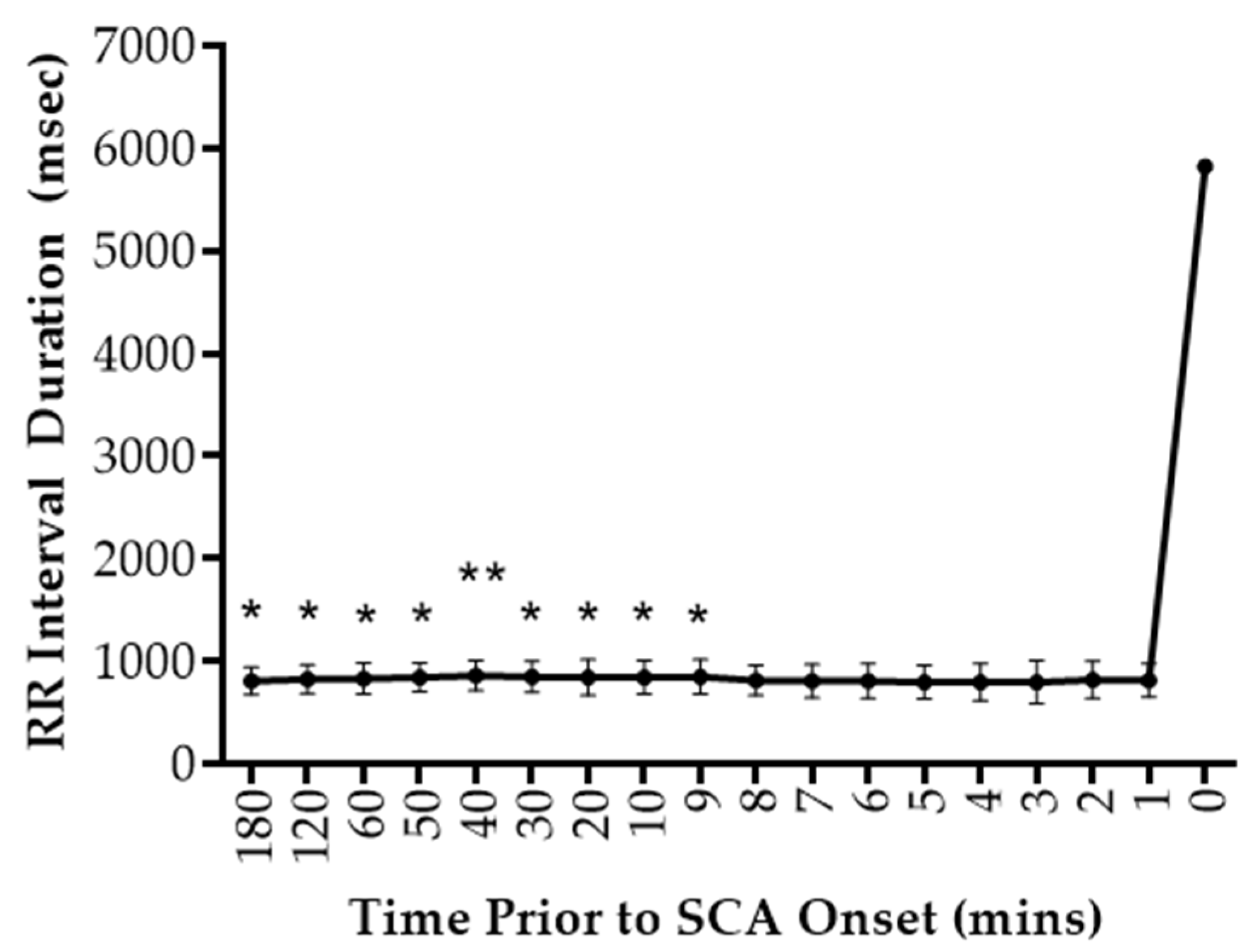
Similarly, the heart rate of patients in the SCA cohort exhibited a higher mean R-R interval duration compared to the normal patients (See Table A1, Appendix A). The mean R-R duration was observed to fluctuate in a similar fashion to heart rate prior to the onset of SCA before exhibiting a sudden increase between 1 min prior to SCA and during the onset of SCA (See Figure 5). There was a statistically significant difference in the mean R-R interval duration at 3 h, F(1,18) = 4.57, p = 0.05, 2 h F(1,18) = 2.72, p = 0.03, 1 h, F(1,18) = 5.34, p = 0.03, 50 min, F(1,18) = 6.88, p = 0.02 , 40 min, F(1,18) = 8.50, p = 0.01, 30 min, F(1,18) = 7.09, p = 0.02, 20 min, F(1,18) = 5.41, p = 0.03, 10 min, F(1,18) = 5.89, p = 0.03 and 9 min, F(1,18) = 5.79, p = 0.03 prior to SCA onset (See Table A2, Appendix B). Post-hoc analyses using Tukey’s HSD indicated that mean R-R interval duration was significantly higher in the SCA patient cohort compared to the normal patient cohort (See Table A4, Appendix B).

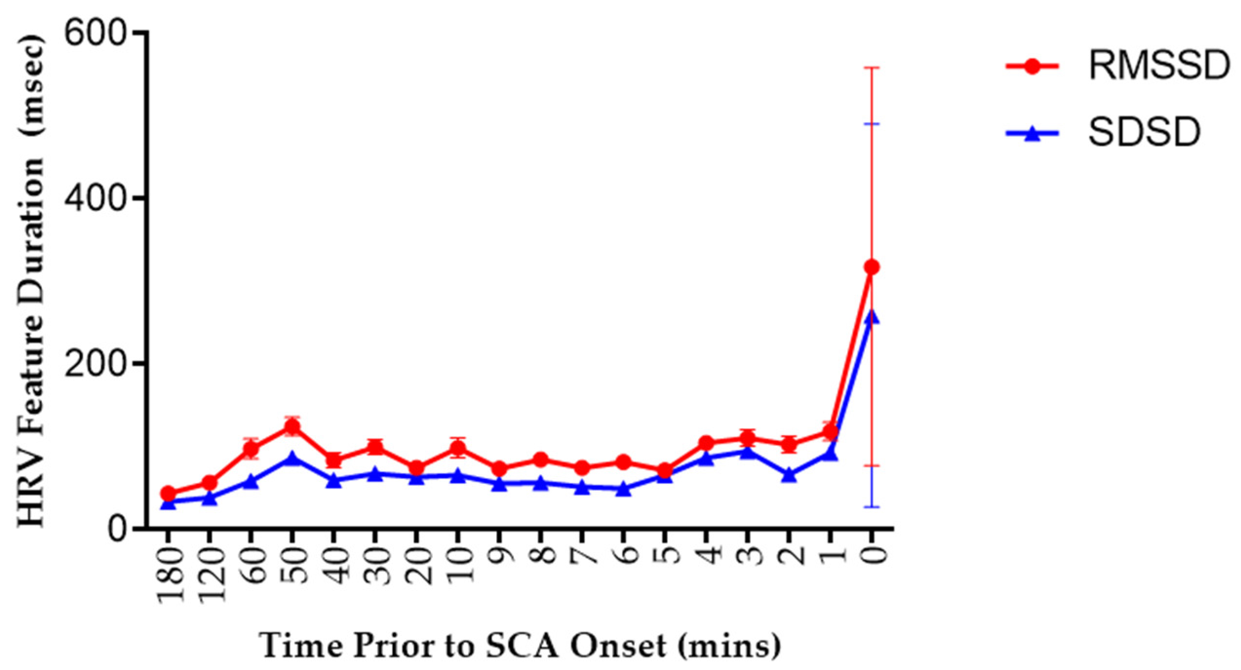
For the HRV features, both the RMSSD and SDSD obtained from the SCA cohort were larger compared to the normal cohort (See Table A1, Appendix A). There was gradual increase in RMSSD observed which peaked at 50 min prior to SCA before fluctuating in a similar fashion to heart rate and R-R interval duration. Similarly, SDSD was observed to fluctuate prior to the onset of SCA, peaking at 3 min prior to SCA. Both RMSSD and SDSD, then exhibited a sudden increase between 1-min prior and during the onset of SCA (See Figure 6). There was a statistically significant difference in RMSSD observed at 3 min prior to SCA between normal and SCA patients, F(1,18) = 4.28, p = 0.05 (See Table A2, Appendix B). However, post-hoc analysis using Tukey’s HSD indicated that there was no significant difference in RMSSD observed between the two patient cohorts (p = 0.05) (See Table A4, Appendix B). There was no statistically significant difference in SDSD observed at any time point between normal and SCA patients (See Table A1, Appendix A).

3.2. Classifier Selection and Statistical Significance

Linear discriminant analysis was first conducted in order to statistically classify patients based on the R-R-interval derived features (mean R-R interval duration, RMSSD, and SDSD) obtained at each time-frame before SCA onset. The best accuracy was obtained at 8 min prior to SCA which exhibited an accuracy of 72.8%. On the other hand, the earliest time-frame which exhibited the best accuracy was 30 min, which produced an accuracy rate of 72.3%. The highest sensitivity was exhibited at 20 min prior with a rate of 70.2%, while the highest specificity rate was observed at 3 min prior at a rate of 83.8% (See

Table 1. Tabular summary of the accuracy, sensitivity, and specificity of the linear classifier.

Time Period	Accuracy	Sensitivity	Specificity
3 h prior	56.7%	49.7%	68.8%
2 h prior	61.5%	55.5%	67.5%
1 h prior	68.3%	59.5%	76.7%
50 min prior	67.0%	55.3%	78.7%
40 min prior	72.2%	68.8%	75.5%
30 min prior	72.3%	69.0%	75.7%
20 min prior	71.3%	70.2%	72.3%
10 min prior	70.8%	63.8%	77.7%
9 min prior	69.8%	62.8%	76.8%
8 min prior	72.8%	70.0%	75.7%
7 min prior	71.4%	65.3%	77.5%
6 min prior	68.8%	64.7%	72.8%
5 min prior	68.5%	61.8%	71.2%
4 min prior	70.3%	64.5%	76.2%
3 min prior	70.7%	57.5%	83.8%
2 min prior	71.1%	62.3%	79.8%
1 min prior	68.5%	57.8%	79.2%

).

Two support vector machine (SVM) classifiers were implemented in this study: linear SVM and a non-linear fine Gaussian SVM. For the linear SVM. The highest accuracy was obtained at two time-frames: 10 min and 8 min prior, both of which exhibited an accuracy rate of 78.9%. The earliest time-frame with reasonable accuracy was at 40 min, which exhibited a rate of 77.1%. The highest sensitivity was exhibited at 8 min prior with a rate of 83.2%, while the highest specificity rate was exhibited at 50 min prior with a rate of 79.0% (See

Table 2. Tabular summary of the accuracy, sensitivity, and specificity of the support vector machine classifiers (SVM): linear SVM and a non-linear Fine Gaussian SVM.

	Linear SVM			Non-Linear SVM
Time Period	Accuracy	Sensitivity	Specificity	Accuracy	Sensitivity	Specificity
3 h prior	61.8%	50.5%	73.5%	78.4%	75.8%	80.2%
2 h prior	68.7%	63.7%	73.7%	77.8%	84.3%	71.2%
1 h prior	75.3%	73.5%	76.0%	77.1%	77.5%	76.2%
50 min prior	76.3%	73.7%	79.0%	80.6%	78.7%	82.5%
40 min prior	77.1%	76.5%	76.5%	78.0%	79.5%	76.5%
30 min prior	76.5%	77.3%	75.7%	77.3%	77.3%	77.2%
20 min prior	73.8%	70.2%	72.3%	76.3%	85.8%	66.8%
10 min prior	78.9%	79.3%	78.5%	82.3%	86.0%	78.5%
9 min prior	77.4%	78.2%	76.7%	81.2%	86.7%	75.7%
8 min prior	78.9%	83.2%	74.7%	80.7%	85.0%	76.3%
7 min prior	71.4%	77.2%	75.2%	78.7%	80.8%	76.5%
6 min prior	74.8%	75.5%	74.0%	78.6%	80.5%	76.7%
5 min prior	74.2%	76.5%	71.8%	78.5%	86.0%	71.0%
4 min prior	74.9%	74.7%	75.2%	78.5%	82.0%	75.0%
3 min prior	76.8%	75.0%	78.5%	82.6%	84.2%	81.0%
2 min prior	78.5%	79.3%	77.7%	83.9%	91.5%	76.3%
1 min prior	75.6%	75.8%	75.3%	81.2%	87.2%	75.2%

). For the non-linear SVM, the highest accuracy was obtained at 2 min prior, which exhibited an accuracy rate of 83.9%. The earliest time-frame with reasonable accuracy was at 50 min prior, which had a rate of 80.6%. The highest sensitivity was exhibited at 2 min prior with a rate of 91.5% while the highest specificity was observed at 50 min prior with a rate of 82.5% (See Table 2).

Across all classifiers, the time-frames that yielded the best accuracy rates were 2 min and 8 min prior to SCA. The earliest time-frames that exhibited the best accuracy rates relative to adjacent time-frames across all classifiers were 50 min and 40 min prior to SCA (See Table 1 and Table 2).

4. Discussion

As the early detection of SCA is critical, yet not well established, the overall intention of this study was to determine the earliest time-frame prior to the onset of SCA in which ECG changes pertaining to SCA can be detected. Statistical comparison of the importance of each feature in comparison to a normal patient population, with a focus on time-based detection was also pertinent to this study.

Heart Rate. The first feature investigated in this study was mean resting heart rate, where patients in the SCA cohort exhibited a higher mean resting heart rate compared to the normal patient cohort. This correlated with literature findings, however, a larger difference between the SCA and normal cohort was observed in this study compared to previously conducted studies (18.9 vs. 7.5 bpm increase in the SCA cohort) [22]. The mean heart rate was then found to gradually increase and decrease between 3 h prior to SCA onset before exhibiting a sudden drop during SCA onset. There was a statistically significant difference in the mean resting heart rate observed between the two cohorts at 3 h and 6 min prior to SCA onset. However, after further statistical analysis statistical significance was only achieved at 3 h prior to SCA onset and as the p-value obtained was close to the cutoff value of 0.05, the findings should be considered as only marginally significant.

The mean resting heart rate is an important marker as it both contributes to and reflects cardiovascular pathophysiology [23]. Heart rate is controlled by neural influences, where under normal physiological conditions the resting heart is under parasympathetic control, as proven in studies involving the pharmacological blockade of the autonomic influences with atropine [24]. The initial increase in heart rate observed occurs as a result of the patient’s underlying cardiovascular disease, where there is a chronic imbalance between the sympathetic and parasympathetic control of the heart. The late decrease observed just prior to SCA onset may be attributed to two mechanisms. The first suggested mechanism is vagal withdrawal, which occurs as a result of contraction-perfusion mismatch and, consequently missed baroreflex input. A high heart rate results in a decrease in the diastolic perfusion time resulting in hemodynamically-insufficient ventricular contractions [25]. Overall, it leads to deleterious effects on the overall cardiac output and ultimately results in hemodynamic collapse and the functional deterioration of the heart. The second suggested mechanism is due to premature ventricular contraction-mediated disturbance of the cardiac cycle. The increased sympathetic output due to CVD results in the heightened electrical instability of the heart. This in turn gives rise of premature ventricular contractions (PVC), which are early depolarizations originating from the ventricle [26]. PVCs result in the delayed activation of the ventricular myocardium as depolarizations from the sinoatrial node are unable to reach the ventricles. As a result, there is a full compensatory pause before the next successive heartbeat following a PVC which, in turn, may contribute to the late decrease in heart rate [27].

It has been widely reported across various large cohort studies, such as the Framingham heart study, that a higher mean resting heart rate is associated with an increase in cardiovascular mortality. Studies have exhibited that an increase in SCA risk was observed in heart rates exceeding 75 bpm [14,22,27]. However, the mechanisms underlying the relationship between elevated resting heart rate and SCA risk are still poorly understood and remain to be elucidated.

Mean R-R Interval Duration. In a similar fashion to resting heart rate, the mean R-R interval duration was longer in SCA patients compared to normal patients. This observation aligns with early studies conducted on ambulatory ECGs of SCA patients, where long R-R interval cycles ranging between 640–1110 ms were observed in approximately 90% of patients prior to SCA [14,28]. These studies have suggested that this prolongation in the R-R interval observed during SCA occurs as a result of PVCs. As stated in the preceding section, PVCs are followed by a full compensatory pause as the depolarizations from the sinoatrial node fail to reach the ventricles [14]. This, consequently, results in disturbances in the cardiac cycle, characterized by the shortening followed by the lengthening of the R-R cycle intervals [29]. These early studies have also exhibited that the frequency of PVCs increase significantly from 1-h prior to SCA until the onset of SCA, which may explain the statistically significant differences in the mean R-R interval duration observed between a single time-frame prior to SCA and SCA onset observed in 50% of the SCA cohort [14,28]. It is also important to consider that external factors, such as the patient’s underlying etiology and medication, may also contribute to R-R interval prolongation.

Heart Rate Variability (RMSSD and SDSD). The final two features investigated in this study were two time-domain measures of heart rate variability (HRV); the square root of the mean of differences between adjacent R-R intervals (RMSSD) and the standard deviation of the differences between adjacent R-R intervals (SDSD). Studies have shown that beat-to-beat changes in the R-R interval may accurately reflect any variability in sinoatrial node activity and features that utilize the difference between adjacent R-R intervals are ideal for long term measurements of HRV [30]. Both the RMSSD and the SDSD of the SCA cohort obtained in this study were higher compared to the normal cohort, although not to a statistically significant extent. Since these features utilize the R-R interval, the difference observed between the SCA and normal patient cohort may be attributed to the mechanisms related to the increase in PVC frequency, as previously discussed in the preceding section. However, the values obtained in this study do not correlate with literature findings which found lower HRV indices in SCA patients [19]. Other literature studies have associated low HRV values as a marker of cardiac dysfunction, while high HRV on the other hand is associated with efficient cardiac autonomic mechanisms [31,32]. Thus, a high HRV index while the patient is at rest is deemed favorable as it indicates that the body is either able to tolerate stress or is strongly recovering from prior accumulated stress [32]. However, it is important to note that a majority of patients in the SCA cohort possess underlying cardiovascular conditions and, as the patients in this study are older than the normal cohort, their hearts have been exposed to stress for a period of time. As a result, their heart may have already acclimatized to these stressful conditions, thus resulting in the high HRV values.

Statistical Classification and Machine Learning. The data was then subjected to statistical classification with the use of various classifiers. The first classifier tested was the linear classifier, which utilized linear discriminant analysis. The best accuracy was yielded at 8 min prior to SCA onset and was found to correlate with literature findings [33,34]. However, the values obtained in this study were slightly lower than the values obtained in similarly-conducted studies (72.80% vs. 74.36%) [33]. This may be attributed to the signal quality, as the accuracy of a classifier depends on two factors; signal quality and the extracted features [35]. SVM classification was then conducted on the dataset and there was an improvement in the accuracy values obtained for both the linear and non-linear SVM classifiers, both of which yielding higher accuracy rates compared to the linear classifier (72.8% vs. 78.9% both obtained at the 8 min prior time-frame). The values obtained from the non-linear SVM classifier were found to correlate with findings obtained from a similar study conducted using the same two ECG database, although the findings obtained for accuracy (83.9% vs. 88.0%), sensitivity (91.5% vs. 92.0%), and specificity (82.5% vs. 84.0%) were slightly lower compared to the literature [34]. This slight variation in values may be due to interpatient variation, as in the literature only five patients each were used for the normal and SCA cohort, whereas the cohort numbers in this study were almost double for both the normal and SCA population.

As time starts to approach the onset of SCA, the overall risk of SCA increases and, thus, the percentage at which the classifier will correctly classify a patient at risk of SCA would consequently increase [19]. Overall, the experimental results exhibited an increase in accuracy with each time window approaching SCA onset, particularly in the findings obtained from the non-linear SVM classifier.

The performance of each classifier based on the isolated time-frames were then quantitatively evaluated by calculating the area under the receiver operating characteristic (ROC) curve. The higher the AUC, the better the classifier performance [36]. The highest overall AUC was obtained by the non-linear SVM classifier in the 2-min time-frame which exhibited an AUC of 0.88. However, there is an approximately 0.02 difference observed between the early time-frames (50 and 40 min prior) and the later time-frames (8 and 2 min prior), suggesting that the risk of SCA can be detected at an earlier time-frame with reasonable accuracy (See

Table 3. Area under the receiver operating characteristic (ROC) curves generated for each classifier.

Classifier	50 Min Prior	40 Min Prior	8 Min Prior	2 Min Prior
Linear (LDA)	0.76	0.79	0.79	0.77
Linear SVM	0.79	0.82	0.81	0.80
Non-Linear SVM	0.86	0.86	0.86	0.88

). Overall, the non-linear SVM had the best performance across all time-frames compared to its linear counterparts, which may be due to the fact that it takes into account the non-linearity of ECG signals.

Across all three classifiers, the highest overall accuracy was obtained at 2 min prior to SCA onset. This is a time-frame in which a significant difference between the ECG recordings obtained from a patient at risk of SCA differing from a normal patient would be expected. This is due to the increase in the frequency of PVCs over time. Thus, more frequent PVCs at 2 min prior would result in larger compensatory pauses which, in turn, affects the HRV features of patients at risk of SCA, resulting in higher accuracies in classifying SCA and normal patients. A similar conclusion was made across various similarly conducted studies which also discovered that the 2-min time window provided the most useful information for SCA detection [19,33,34,35]. However, it is important to note that the overall aim of SCA detection is to identify patients at risk as early as possible in order to prevent serious repercussions, such as irreversible neurological damage, and even death. Thus, 2 min prior to the onset of SCA is not enough time to allow a patient to respond and seek management.

However, it was also observed that reasonable accuracy rates of 70–80% can be obtained across all three classifiers as early as 50 min prior to the onset of SCA. This, in turn, may provide sufficient time for a patient to respond and reach the hospital to immediately undergo SCA management, in turn reducing the risk of serious complications such as neurological damage, organ failure and, most importantly, death. These time-frames, however, are yet to be explored in the current literature as time-frames spanning only up to 5 min prior to SCA onset have been explored, which does not provide sufficient time for optimal patient response.

5. Conclusions

The present study explored the detection of SCA through the statistical comparison of ECG features, such as heart rate and R-R interval related markers, between normal and patients at risk of SCA and the identification of the ideal time-frame for detection spanning up to three hours prior to the onset of SCA. Overall, there was a statistically significant change in heart rate 3 h and 6 min prior to SCA onset. There was also a statistically significant change in R-R interval duration the observed 9 min to 3 h prior to SCA onset and for RMSSD at 3 min. Conversely, there was no statistically significant change observed in SDSD at any time-frame. Following classification, the 2-min time-frame exhibited the highest accuracy across all three classifiers. However, reasonable accuracies were obtained at the 40 and 50-min time-frames which, in turn, may provide sufficient time for optimal patient response. The main limitation presented in this study was the small cohort numbers. As only 10 patients were used in each cohort, this may have attributed to the low performance measurement values. This can be addressed through further testing on a larger cohort prior to clinical application. Future studies may also aim to explore ECG feature detection specifically in the SCA patient cohort through the analysis and comparison of time-frames prior to, during, and possibly after the onset of SCA. Overall, the present study further contributes to the growing field of SCA detection by analyzing time-frames three hours prior to SCA onset, in which clinically-useful information can be obtained and utilized in the clinical setting to improve overall patient survival.

References

- Zipes, D.P.; Wellens, H.J. Sudden cardiac death. Circulation 1998, 98, 2334–2351. [Google Scholar] [CrossRef] [PubMed]
- Yousuf, O.; Chrispin, J.; Tomaselli, G.F.; Berger, R.D. Clinical management and prevention of sudden cardiac death. Circ. Res. 2015, 116, 2020–2040. [Google Scholar] [CrossRef] [PubMed]
- Israel, C.W. Mechanisms of sudden cardiac death. Indian Heart J. 2014, 66, S10–S17. [Google Scholar] [CrossRef] [PubMed]
- Estes, N.M. Predicting and preventing sudden cardiac death. Circulation 2011, 124, 651–656. [Google Scholar] [CrossRef] [PubMed]
- Australian Resuscitation Council New South Wales (ARC NSW). Cardiac Arrest—An Introduction. 2016. Available online: http://www.aeds.com.au/blog/what-is-sudden-cardiac-arrest (accessed on 20 February 2017).
- Graham, R.; McCoy, M.A.; Schultz, A.M. Strategies to Improve Cardiac Arrest Survival: A Time to Act; Institute of Medicine Report; The National Academies Press: Washington, DC, USA, 2015. [Google Scholar]
- Wellens, H.J.; Schwartz, P.J.; Lindemans, F.W.; Buxton, A.E.; Goldberger, J.J.; Hohnloser, S.H.; Huikuri, H.V.; Kääb, S.; La Rovere, M.T.; Malik, M. Risk stratification for sudden cardiac death: Current status and challenges for the future. Eur. Heart J. 2014, 35, 1642–1651. [Google Scholar] [CrossRef] [PubMed] [Green Version]
- Tamene, A.; Tholakanahalli, V.N.; Chandrashekhar, Y. Cardiac imaging in evaluating patients prone to sudden death. Indian Heart J. 2014, 66 (Suppl. 1), S61–S70. [Google Scholar] [CrossRef] [PubMed]
- Thomas, K.E.; Josephson, M.E. The role of electrophysiology study in risk stratification of sudden cardiac death. Prog. Cardiovasc. Dis. 2008, 51, 97–105. [Google Scholar] [CrossRef] [PubMed]
- Goyal, V.; Jassal, D.S.; Dhalla, N.S. Pathophysiology and prevention of sudden cardiac death. Can. J. Physiol. Pharmacol. 2016, 94, 237–244. [Google Scholar] [CrossRef] [PubMed]
- Lewis, B.H.; Antman, E.M.; Graboys, T.B. Detailed analysis of 24 hour ambulatory electrocardiographic recordings during ventricular fibrillation or torsade de pointes. J. Am. Coll. Cardiol. 1983, 2, 426–436. [Google Scholar] [CrossRef]
- Panidis, I.P.; Morganroth, J. Sudden death in hospitalized patients: Cardiac rhythm disturbances detected by ambulatory electrocardiographic monitoring. J. Am. Coll. Cardiol. 1983, 2, 798–805. [Google Scholar] [CrossRef]
- Pratt, C.M.; Francis, M.J.; Luck, J.C.; Wyndham, C.R.; Miller, R.R.; Quinones, M.A. Analysis of ambulatory electrocardiograms in 15 patients during spontaneous ventricular fibrillation with special reference to preceding arrhythmic events. J. Am. Coll. Cardiol. 1983, 2, 789–797. [Google Scholar] [CrossRef]
- De Luna, A.B.; Coumel, P.; Leclercq, J.F. Ambulatory sudden cardiac death: Mechanisms of production of fatal arrhythmia on the basis of data from 157 cases. Am. Heart J. 1989, 117, 151–159. [Google Scholar] [CrossRef]
- Barletta, V.; Fabiani, I.; Lorenzo, C.; Nicastro, I.; Bello, V.D. Sudden cardiac death: A review focused on cardiovascular imaging. J. Cardiovasc. Echogr. 2014, 24, 41–51. [Google Scholar] [PubMed]
- Sansone, M.; Fusco, R.; Pepino, A.; Sansone, C. Electrocardiogram pattern recognition and analysis based on artificial neural networks and support vector machines: A review. J. Healthc. Eng. 2013, 4, 465–504. [Google Scholar] [CrossRef] [PubMed]
- Balli, T.; Palaniappan, R. Classification of biological signals using linear and nonlinear features. Physiol. Meas. 2010, 31, 903–921. [Google Scholar] [CrossRef] [PubMed]
- Goldberger, A.L.; Amaral, L.A.; Glass, L.; Hausdorff, J.M.; Ivanov, P.C.; Mark, R.G.; Mietus, J.E.; Moody, G.B.; Peng, C.K.; Stanley, H.E. Physiobank, physiotoolkit and physionet: Components of a new research for complex physiologic signals. Circulation 2000, 101, e215–e220. [Google Scholar] [CrossRef] [PubMed]
- Ebrahimzadeh, E.; Pooyan, M.; Bijar, A. A novel approach to predict sudden cardiac death (SCD) using nonlinear and time-frequency analyses from hrv signals. PLoS ONE 2014, 9, e81896. [Google Scholar] [CrossRef] [PubMed]
- Song, M.H.; Lee, J.; Cho, S.P.; Lee, K.J.; Yoo, S.K. Support vector machine based arrhythmia classification using reduced features. Int. J. Control Autom. Syst. 2005, 3, 571–579. [Google Scholar]
- Nuryani, N.; Harjito, B.; Yahya, I.; Solikhah, M.; Chai, R.; Lestari, A. Atrial fibrillation detection using support vector machine and electrocardiographic descriptive statistics. Int. J. Biomed. Eng. Technol. 2017, 24, 225–236. [Google Scholar] [CrossRef]
- Teodorescu, C.; Reinier, K.; Uy-Evanado, A.; Gunson, K.; Jui, J.; Chugh, S.S. Resting heart rate and risk of sudden cardiac death in the general population: Influence of left ventricular systolic dysfunction and heart rate-modulating drugs. Heart Rhythm 2013, 10, 1153–1158. [Google Scholar] [CrossRef] [PubMed]
- Arnold, J.M.; Fitchett, D.H.; Howlett, J.G.; Lonn, E.M.; Tardif, J.-C. Resting heart rate: A modifiable prognostic indicator of cardiovascular risk and outcomes? Can. J. Cardiol. 2008, 24, 3A–15A. [Google Scholar] [CrossRef]
- La Rovere, M.T. Heart Rate and Arrhythmic Risk: Old Markers Never Die; European Heart Rhythm Association: Antipolis, France, 2010. [Google Scholar]
- Bauer, A.; Malik, M.; Schmidt, G.; Barthel, P.; Bonnemeier, H.; Cygankiewicz, I.; Guzik, P.; Lombardi, F.; Müller, A.; Oto, A. Heart rate turbulence: Standards of measurement, physiological interpretation, and clinical use: International society for holter and noninvasive electrophysiology consensus. J. Am. Coll. Cardiol. 2008, 52, 1353–1365. [Google Scholar] [CrossRef] [PubMed]
- Ahn, M.-S. Current concepts of premature ventricular contractions. J. Lifestyle Med. 2013, 3, 26. [Google Scholar] [PubMed]
- Kannel, W.B.; Kannel, C.; Paffenbarger, R.S.; Cupples, L.A. Heart rate and cardiovascular mortality: The framingham study. Am. Heart J. 1987, 113, 1489–1494. [Google Scholar] [CrossRef]
- Denes, P.; Gabster, A.; Huang, S.K. Clinical, electrocardiographic and follow-up observations in patients having ventricular fibrillation during holter monitoring: Role of quinidine therapy. Am. J. Cardiol. 1981, 48, 9–16. [Google Scholar] [CrossRef]
- Guzik, P.; Schmidt, G. A phenomenon of heart-rate turbulence, its evaluation, and prognostic value. Card. Electrophysiol. Rev. 2002, 6, 256–261. [Google Scholar] [CrossRef] [PubMed]
- Kamath, M.V.; Watanabe, M.A.; Upton, A. Heart Rate Variability (HRV) Signal Analysis: Clinical Applications; CRC Press: Boca Raton, FL, USA, 2012. [Google Scholar]
- Draghici, A.E.; Taylor, J.A. The physiological basis and measurement of heart rate variability in humans. J. Physiol. Anthropol. 2016, 35, 22. [Google Scholar] [CrossRef] [PubMed]
- Stein, P.K.; Bosner, M.S.; Kleiger, R.E.; Conger, B.M. Heart rate variability: A measure of cardiac autonomic tone. Am. Heart J. 1994, 127, 1376–1381. [Google Scholar] [CrossRef]
- Ebrahimzadeh, E.P.M. Early detection of sudden cardiac death by using classical linear techniques and time-frequency methods on electrocardiogram signals. J. Biomed. Sci. Eng. 2011, 4, 699–706. [Google Scholar] [CrossRef]
- Sheela, C.J.; Vanitha, L. Prediction of sudden cardiac death using support vector machine. In Proceedings of the 2014 International Conference on Circuit, Power and Computing Technologies, Nagercoil, India, 20–21 March 2014. [Google Scholar]
- Ripoll, V.J.R.; Wojdel, A.; Romero, E.; Ramos, P.; Brugada, J. ECG assessment based on neural networks with pretraining. Appl. Soft Comput. 2016, 49, 399–406. [Google Scholar] [CrossRef]
- Chai, R.; Naik, G.R.; Nguyen, T.N.; Ling, S.H.; Tran, Y.; Craig, A.; Nguyen, H.T. Driver fatigue classification with independent component by entropy rate bound minimization analysis in an EEG-based system. IEEE J. Biomed. Health Inform. 2017, 21, 715–724. [Google Scholar] [CrossRef] [PubMed]
Figure 1.
Block diagram of the methodology.
Figure 2.
Block diagram of the data segmentation process for the ECG recordings obtained from the SCA cohort.
Figure 3.
Raw double channel ECG signal, raw single channel ECG signal prior to pre-processing and ECG signal after pre-processing with baseline wander removal.
Figure 4.
Time series plot of the change in heart rate prior to the onset of sudden cardiac arrest (n = 10). ECG recordings were taken from patients in the SCA cohort and subjected to processing via MATLAB. The results were recorded as mean heart rate (±standard deviation) denoted by the error bars. The asterisk denotes the statistical significance by repeated measures ANOVA where * p < 0.05.
Figure 5.
Time series plot of the change in R-R Interval duration prior to the onset of sudden cardiac arrest (n = 10). ECG recordings were taken from patients in the SCA cohort and subjected to processing via MATLAB. The results were recorded as mean R-R interval duration (±standard deviation) denoted by the error bars. Asterisks denote statistical significance by repeated measures ANOVA where * p < 0.05 and ** p < 0.01.
Figure 6.
Time series plot of the changes in heart rate variability (HRV): the square root of the mean of differences between all adjacent R-R intervals (RMSSD) and the standard deviation of differences between all adjacent R-R intervals (SDSD) (n = 10). ECG recordings were taken from patients in the SCA cohort and subjected to processing via MATLAB. The results were recorded as mean RMSSD (±standard deviation) and SDSD (±standard deviation) denoted by the error bars.