Portfolio Implementation Risk Management Using Evolutionary Multiobjective Optimization


1
Department of Computer Science, Universidad Carlos III de Madrid, Madrid 28911, Spain
2
IPC—Institute of Polymers and Composites, University of Minho, Campus de Azurém, 4800-058 Guimarães, Portugal
3
CEA, LIST, Data Analysis and System Intelligence Laboratory, 91191 Gif-sur-Yvette, France
*
Author to whom correspondence should be addressed.
†
Current address: Department of Computer Science, Universidad Carlos III de Madrid, Av. de la Universidad 30, Leganés, 28911 Madrid, Spain.
Appl. Sci. 2017, 7(10), 1079; https://0-doi-org.brum.beds.ac.uk/10.3390/app7101079
Submission received: 11 September 2017
/
Accepted: 12 October 2017
/
Published: 18 October 2017
Abstract
:Portfolio management based on mean-variance portfolio optimization is subject to different sources of uncertainty. In addition to those related to the quality of parameter estimates used in the optimization process, investors face a portfolio implementation risk. The potential temporary discrepancy between target and present portfolios, caused by trading strategies, may expose investors to undesired risks. This study proposes an evolutionary multiobjective optimization algorithm aiming at regions with solutions more tolerant to these deviations and, therefore, more reliable. The proposed approach incorporates a user’s preference and seeks a fine-grained approximation of the most relevant efficient region. The computational experiments performed in this study are based on a cardinality-constrained problem with investment limits for eight broad-category indexes and 15 years of data. The obtained results show the ability of the proposed approach to address the robustness issue and to support decision making by providing a preferred part of the efficient set. The results reveal that the obtained solutions also exhibit a higher tolerance to prediction errors in asset returns and variance–covariance matrix.
1. Introduction
The problem of identifying the best potential combinations of assets has been present in the academic financial literature for a long time. Among the efforts made, the seminal framework introduced by Harry Markowitz [1,2] has been especially influential. Markowitz suggested analyzing sets of assets, also known as financial portfolios, in terms of risk and return. These two issues are contradictory in nature, since the desired higher returns usually come at a price of higher risks. The portfolio selection problem formulated by Markowitz addresses the minimization of portfolio return variance subject to a minimum expected value of return. The best combinations of assets for certain degrees of risk define a line, the efficient frontier. Portfolios along this line have the best properties as, for each level or risk, there is no alternative that offers a higher return. Under some assumptions, these combinations can be identified by repeated use of quadratic programming.
Unfortunately, simplistic assumptions of the classical Markowitz model usually do not hold in the real world. Problems faced by practitioners might include complex constraints or definitions of risk that differ from the canonical portfolio standard deviation of returns, among others. For this reason, there has been a need to find alternative ways to handle the optimization process.
Among the recent advances in optimization algorithms [3], evolutionary algorithms (EAs) have proven successful in overcoming difficulties with traditional optimization techniques either in their standard version, or hybridized [4,5,6].
EAs work with a set of solutions, called population. This feature is particularly suitable for solving multiobjective problems, as it enables approximating the efficient frontier in a single run. As a result, multiobjective evolutionary algorithms (MOEAs) have received growing attention to financial applications [7]. In fact, portfolio optimization was one of the first successful applications of MOEAs in economics and finance. The body of literature devoted to the topic has grown significantly over the last years [8]. The interest in the general subject, stronger than ever, can be illustrated by recent innovations on algorithms [9,10,11] and evolutionary operators [12]. However, the problem of robustness has been subject to a much lower amount of research.
In the context of mean-variance portfolio optimization, the term of robustness can refer to different sources of uncertainty, such as the accuracy of future asset returns or the nature of the variance–covariance matrix [13,14]. The portfolio performance will not be optimal if incorrect parameter values are used. The risk due to parameter uncertainty is commonly referred to as estimation risk. Another source of uncertainty is portfolio implementation risk. With the latter, we make reference to the possibility of temporary deviations form a target allocation that could result in undesired exposure. The aim of this paper is to show how to limit this problem by means of a robustness-based S-metric evolutionary multiobjective optimisation algorithm [15] (SMS-EMOA).
As of today, most of the efforts made to mitigate uncertainty during the optimization process have been focused on parameters and the ability of the solutions to tolerate a certain degree of noise. Some examples of these efforts are [16,17,18]. Among the few works that deal with this issue using evolutionary algorithms, we can mention some that rely on the basic principle of picking solutions based on a number of future potential scenarios instead of a single prediction. For instance, in [19], profitable trading strategies are found by means of genetic programming. In [20], a portfolio modeling approach that considers uncertainty in returns of risky asset is presented and solved with a genetic algorithm (GA).
We can also mention [21], which plays with modifications and extensions of common robust optimization techniques by using an hybrid heuristic as solver, or [22], that introduces a single/multiobjective inverse robust evolutionary approach based on non-probabilistic methods that tries to deal with uncertainty in parameters. Lastly, in [23], the authors explored the possibility of increasing the robustness of the solutions obtained by a multiobjective genetic algorithm, exposing the system to several markets.
On the other hand, in [24,25], the focus is more on the single-period portfolio optimization problem described above. In [26], a time-stamped resampling strategy is introduced along with a variant that extends the basic two-objective framework by explicitly adding a third robustness objective. A similar problem is tackled in [27] by a different strategy for a multiperiod setup. More specifically, the integration of an anticipatory learning method using Kalman Filters is proposed. However, the scenario considered in this work is different.
When asset managers identify allocations of interest, the process of rebalancing existing portfolios or creating new ones is not always immediate. Once the decision regarding the target portfolio has taken, some considerations should be made before implementation. Is the market deep enough to meet the order at current price or is likely to move prices? Is it desirable to conceal temporarily the structure of the target portfolio? Similar questions might result in different trading strategies, some of which require building the desired position over time. During this period, especially in the later stages, the portfolio will be similar to the chosen one, but different. This deviation in the structure can result in properties in terms of risk and return that differ from the expected one. If the intermediate portfolio is especially sensitive, this can lead to undesired risk exposure. In this view, a portfolio would be considered robust to implementation risk if small deviations in its composition result in similar risk–return profiles.
This desirable trait for portfolios is closely related to robust design optimization focusing on finding solutions that are reliable under given uncertainties. There are two closely related aspects: the feasibility and performance robustness. The robustness against performance deterioration is referred as to the performance robustness. It can be addressed either by optimizing the expectation and variance [28,29] or by introducing additional constraints [28]. Different types of robustness measures for multiobjective optimization were investigated in [30]. A methodology for incorporating the robustness measure into fitness values of population members in MOEAs were developed in [31]. On the other hand, the robustness of solutions against failure is a subject of reliability-based optimization techniques. They usually address a stochastic optimization problem in which the constraints are converted into probabilistic constraints. The probability of a solution being feasible is determined by a reliability index. The solution reliability can be determined by either a Monte Carlo simulation that generates a number of samples and estimates the probability of failure or optimization-based procedures that estimate the distance from the solution to the constraint [32]. For good surveys on robust optimization, an interested reader is kindly referred to [33,34].
This study follows the methodology developed in [31] and suggests a robustness-based S-metric selection evolutionary multiobjective optimization algorithm (R-SMS-EMOA) for portfolio optimization to account for inherit uncertainties. The approach also allows the user to express and incorporates a preference information in terms the desirable degree of solutions robustness. This information is used to adjust the optimization and to focus on the most preferred regions of the search space. The experimental results indicate that thereby obtained solutions are more robust with respect to: (i) implementation risk, and (ii) uncertainty in the estimates for future asset returns and variance–covariance matrix (estimation risk).
The rest of the paper is organized as follows. First, in Section 2, we formally describe the financial portfolio optimization problem. In addition to that, we discuss the characterization of implementation risk and the evolutionary multiobjective optimization algorithm to be used. This is followed by the introduction to the sample and the experimental setup. Section 3 will be used to report the results and Section 4 to their discussion. Finally, the last one will be devoted to summary and conclusions.
2. Materials and Methods
We will start this section providing a brief description of the traditional portfolio optimization problem under the Modern Portfolio Theory framework.
2.1. Portfolio Optimization Problem
Markovitz suggested that the aggregate behavior of the components should be analyzed according to two dimensions: risk and return.
Given the linear nature of portfolio structure, the first of them is just the weighted average of the expected return for the assets. Defining risk, however, is more complicated. Markovitz suggested modeling this component through the variance or the standard deviation of returns, bearing in mind that the pattern of returns for the assets included in portfolios could be such that the movements could be negatively correlated, hence providing diversification benefits.
There are different ways to characterize the risk, such as semivariance and expected shortfall. In this work, the risk is determined by the standard deviation of the returns , which is the most prevalent way in the literature.
The problem, therefore, can be considered as multiobjective with two conflicting objectives formally defined as follows.
Maximize total expected return:
Minimize portfolio risk:
subject to:
where n is the number of investment alternatives, is the expected return of the asset i, is the covariance between assets i and j, and are the relative weights of the components of the portfolio that represent the decision variables.
The first constraint, modeled in Equation (3), requires full investment whereas the second, given in Equation (4), prevents the investor from shorting. In addition to that, we will also consider two real world constraints:
Cardinality: there is a maximum and minimum number of assets in which it is possible to invest simultaneously:
where is a binary variable. If asset i is held in the portfolio () the . Otherwise, .
Investment limits: in case an investment alternative is present in the portfolio, its relative weight should be in the interval [, ], where:
The addition of these constraints, especially the cardinality one, increases the complexity of the problem very significantly. In addition to these, investors might be subject others imposed by regulators or internal processes. In this paper, we do not intend to consider all the possible constraints. Given that the set that might be relevant would depend on the specific circumstances of the investor, we just added a few that complicate the basic problem enough to justify the use of heuristics instead of standard quadratic programming.
As we mentioned before, given the multiobjective nature of the problem, the solution is not a single portfolio but a set of them. They define a curve in the risk–return space that represents the dominating portfolios as, for every risk level, no portfolio offers a higher expected return.
It is worth noting that there are several well-known alternatives to characterize portfolio risk. In addition to variance/standard deviation, one could consider value-at-risk, risk of loss, shortfall risk, etc. The algorithm introduced in this paper could work with any of them just as easily. However, we will stick to the most popular characterization for the experimental work.
2.2. Proposed Approach
This subsection presents the details of the proposed multiobjective evolutionary algorithm for a portfolio optimization that uses a robustness-based preference information to focus on a desired regions of the Pareto set. As a core framework for performing the search, SMS-EMOA [15] is selected due to its competitiveness, popularity and frequent use in the literature. In addition, SMS-EMOA has already proven effective in the context of portfolio optimization [35], with both the basic and modified versions being used.
2.2.1. General Framework
SMS-EMOA is a hypervolume-based algorithm with a steady-state selection. It falls into a general framework of evolutionary algorithms, where, after a random initialization, a population of individuals is evolved by successively applying mating selection, variation and environmental selection procedures.
The algorithm starts by randomly generating an initial populating of size N. Each population member is characterized by the decision vector , the objective vector and the robustness measure . Every portfolio is encoded by a vector of real numbers in which each variable represents the percentage of investment per asset. Since there is a set of constraints involved in selecting investment portfolios, each population member must satisfy these constraints in order to represent a feasible investment strategy. Therefore, each time a new individual is generated, it is then repaired to ensure its feasibility. Since the individual reparation procedure is complex, we present a simplified version of it in Algorithm 1.
| Algorithm 1 Reparation |
| 1: Input: , , , , , , |
| 2: while do |
| 3: randomly select i such that |
| 4: |
| 5: end while |
| 6: while do |
| 7: select the smallest of the set |
| 8: |
| 9: end while |
| 10: while do |
| 11: while () or () do |
| 12: if then |
| 13: randomly select i such that |
| 14: |
| 15: end if |
| 16: if then |
| 17: randomly select i such that |
| 18: |
| 19: end if |
| 20: end while |
| 21: if then |
| 22: randomly select i such that |
| 23: introduce to make |
| 24: end if |
| 25: end while |
| 26: Output: |
The mating selection procedure selects two parents for producing an offspring. The selection can be performed in various ways. In the original study [15], two population members are picked uniformly at random from the current population. In this work, a binary tournament selection is used, based on the fitness values of population members, to provide a selection strategy in which fitter individuals have more chance for reproduction, thereby propagating useful characteristics among the population. The fitness assignment strategy, which is a crucial feature of the proposed approach, is described in detail later in this section. The variation procedure recombines two parents by the simulated binary crossover (SBX) [36] followed by applying the polynomial mutation [37]. Since the recombination results in a pair of offspring, one randomly selected offspring is discarded. After the evaluation, the offspring is added to the populating and the environmental selection procedure determines, on the basis of fitness values, which individuals must form the population of the next generation. This is done by removing an individual having the worst fitness value among the population.
2.2.2. Fitness Assignment
Contrary to single-objective optimization, where an individual’s fitness usually results directly from the objective function value, the fitness assignment in multiobjective optimization is not so straightforward as individuals are compared against multiple typically conflicting objectives. Since the fitness is the basis for selection, the effectiveness of any EMO algorithm largely depends on this design issue. Additionally to the convergence and diversity (two primary goals of multiobjective optimization), which must be reflected by the fitness value assigned to each population member, in this study, we propose a fitness assignment strategy that incorporates the robustness issue. The outline of the fitness assignment procedure is shown in Algorithm 2.
| Algorithm 2 Fitness assignment |
| 1: Input: P |
| 2: sort P into non-domination fronts (, , …) |
| 3: |
| 4: for do |
| 5: |
| 6: end for |
| 7: |
| 8: |
| 9: for do |
| 10: for do |
| 11: |
| 12: end for |
| 13: end for |
| 14: for do |
| 15: sort in descending order of |
| 16: sort in ascending order of R |
| 17: for do |
| 18: assign a with based on sort in line 15 |
| 19: assign a with based on sort in line 16 |
| 20: end for |
| 21: end for |
| 22: for do |
| 23: |
| 24: end for |
| 25: Output: P |
The calculation of fitness values involves ranking the population with respect to dominance, diversity and robustness. These ranks are denoted as , and , respectively. An individual’s fitness results from the aggregation of these ranks. The process starts with a fast nondominated sorting procedure [38] that assigns each population member to the corresponding non-domination front (, and so on), according to the Pareto dominance relation. Next, in the first non-domination front , an individual with the best robustness measure is identified (line 3). Thereafter, individuals exhibiting promising characteristics with respect to the robustness are emphasized. To this end, the robustness ratio is calculated for each individual in the first front (lines 4–6). This calculation involves a scaling factor , determined experimentally. Individuals having the robustness ratio lower than the dispersion parameter are retrieved from to form a distinct front . The ranks of the remaining individuals remain unchanged (lines 7–8). This completes the calculation of of each population member.
Afterwards, in each identified front, a hypervolume contribution of each individual is calculated. In line 11, is a metric that measures the amount of the objective space dominated by the set and bounded by the reference point [39]. It can be defined as the Lebesgue measure of the union of hypercuboids in the objective space:
before calculating hypervolume contributions of individuals in the corresponding front, the objective values, to be minimized, are normalized as:
where is the normalized objective value, and are the minimum and maximum objective values of the j-th objective in the corresponding front, respectively. This way, the objective values are mapped into the domain , whereas the reference point is . The extreme points are emphasized by assigning a maximum possible value of .
The fitness assignment procedure calculates ranks for individuals in each front based on the values of hypervolume contribution and robustness R (lines 14–21). The use of rank values allows for coping with different magnitudes of measures incorporated into the fitness. With rank values, it is easy to aggregate the convergence, diversity and robustness measures, regardless of whether increase or decrease in their values leads to a better performance. In the case of , higher values are preferred. Thus, an individual with the largest value of is assigned . Next, the remaining individuals are considered, with being assigned to an individual having the largest value of and so on. On the other hand, lower values of R correspond to more robust solutions. Thus, the ranking based on the robustness measure values is performed in ascending order. An individual with the smallest value of R is assigned , an individual having the second smallest value of R being assigned and so on.
Finally, the global fitness value F is computed for each population member. This is done by aggregating the three ranks as shown in line 23. Thus, the resultant fitness value reflects the quality of a given individual with respect to convergence, diversity and robustness. The extent to which the robustness influences the fitness of population members is determined by the dispersion parameter , which is a control parameter set by the user in the range . Increasing will weak the role of robustness, with the population diversity in the objective making more important. On the contrary, reducing will put more emphasis on the solution robustness. As a result, selection is expected favor more robust individuals and to focus the search on regions with higher robustness of solutions. For , the selection reduces to the original procedure of SMS-EMOA [15], which can be viewed as a particular case of the proposed selection procedure.
The dispersion parameter is an important feature of the proposed approach. It enables the user to express his preferences about the robustness of solutions, thereby determining the focus of the search in advance. This way, a high-grained approximation of the preferred part of the efficient set can be obtained. This is a useful property, as, in practice, many Pareto optimal solutions are not relevant for the decision maker. Typically, the decision maker is only interested in a subset of optimal solutions that exhibit certain characteristics. Moreover, a single solution is eventually selected by incorporating some high-level preferences. By enabling the user to integrate his preferences before the search, the proposed approach aims to support decision-making when determining an optimal strategy for investment in a portfolio of assets.
2.2.3. Internal Robustness Measure
Addressing the issue of robustness requires a formal definition. The measure presented in this study encompasses the variations of the objective functions and the decision variables.
The robustness measure R is formulated as:
with
where and are the j-th variable and objective of the i-th sample point, respectively, is the number of sample points, and refer the j-th variable and objective of population member a.
The robustness measure R estimates how robust a given portfolio is, based on the ratio between the deviations in its neighborhood in the decision and objective spaces. As the objective space is defined by risk and return, the average between two variations is considered, as shown in Equation (11). Since risk is taken as the standard deviation, both risk and expected return deviations are expressed in the same scale. The average value of deviations is also considered for multiple weights in portfolio, as given in Equation (12). The neighborhood of a given portfolio is explored by a number of sample points. The value of R is obtained by averaging over the ratios of deviations, as shown in Equation (10). The smaller the value of R, the more robust the solution.
The estimation of the robustness measure depends largely on the sample of points involved in its calculation. A common approach to sampling consists in generating a number of points in the neighborhood of the given solution. For the portfolio optimization problem, this process is complicated by a set of cardinality constraints that must be satisfied by every sampling point to obtain a feasible portfolio. The outline of the developed sampling procedure is shown in Algorithm 3.
| Algorithm 3 Sampling |
| 1: Input: , , , , , |
| 2: for do |
| 3: if then |
| 4: |
| 5: else if then |
| 6: |
| 7: else |
| 8: |
| 9: end if |
| 10: |
| 11: end for |
| 12: , ensuring |
| 13: Output: |
For every investment greater than zero, the perturbation is performed in a feasible direction. To ensure that the budget constraint 3, the decision vector is projected onto the unit hyperplane, which, in turn, corresponds to a feasible portfolio investment scenario.
2.2.4. Complexity Analysis
The complexity of one generation of the algorithm is governed by the selection procedure. It involves finding the worst fitness value among N population members that takes time. The computation of fitness values involves the nondominated sorting that runs in where all population members are compared with each other with respect to m objectives. In the worse case scenario, all individuals are nondominated. The fitness assignment also involves sorting the hypervolume contributions and robustness values with the time complexity of . When computing the hypervolume contributions for two objectives, the time complexity is governed by the sorting algorithm, which is . In the fitness assignment, the robustness of offspring is estimated by sampling and evaluating points as well as computing deviations for n variables and m objectives. This has the time complexity of and governs the selection procedure because and n are expected to be larger than a population size in the real world scenario. Nonetheless, from the analysis, it can be seen that the overall algorithm remains efficient.
2.3. Data
The experimental analysis is performed to validate the suggested approach. The analysis is based on the evolution of eight broad financial indexes representing different asset classes. The sample covers monthly returns for the time period from January 2000 to December 2014. That is, we rely on 180 monthly returns per series. Table 1 reports the list of indexes and their Datastream mnemonic.
The Russell 1000 Growth Index tracks the growth segment among the US equities with larger capitalization, that is, it is focused on large companies with higher price-to-book ratios and higher expected growth. Conversely, the value index covers companies with lower price-to-book ratios and lower expected growth values. The main difference among these two and the Russel 2000 variants is the size of the companies considered. The latter considers only small-caps. The remaining three track commodities, corporate and government bonds, respectively.
The selection of these indexes is not meant to be a comprehensive representation the universe of investment alternatives, which has much larger scale, but a mere representative set of broad asset categories. The suggested approach can handle significantly larger instances, but, given the number of experiments, we decided to test the performance of the approach on a smaller one.
2.4. Experimental Setup
Given that solving a single optimization problem would not be enough to evaluate the approach, a sliding window is used. This way, instead of using all the data at once to estimate a single vector of future returns and a variance–covariance matrix, we define several subsets of returns for consecutive dates. This creates a number of partially overlapping single-period optimization problems that include a wide range of market conditions that are tackled one by one.
More specifically, we start by defining a 10-year window consisting of the consecutive months between January 2000, , and December 2009, . This data is subsequently used to estimate the parameters required to find the efficient frontier for January 2010, . Once this first problem is solved, we generate a second one that considers to to estimate the vector of returns and the variance–covariance matrix for February 2010, . It is worth noting that the approach is agnostic to the parameter estimation method, as these are part of the problem specification, not the solution strategy. For convenience, we used the standard approach of forecasting returns using the sample average, but the algorithm would be the same if we used Black–Litterman, a perfect forecast, or any other alternative.
The previous process is repeated 60 times to generate 60 different optimization problems, finding the efficient frontiers for the January 2010 to December 2014 period. That is, we define 60 different single-period problem instances using the sliding window. For each of them, we search for the robust efficient frontier relying on training samples of 10 years worth of data. The estimated robust solutions for the following unobserved time period are subsequently assessed.
For each sliding window, 20 independent runs are performed with a population size of , running for function evaluations. The further parameter settings are as follows. The real representation of the decision variables is used. The variation operator involves the SBX crossover and polynomial mutation applied with the probability of and (where n is the number of decision variables), respectively. The crossover and mutation distribution indexes are and , respectively.
Regarding the constraints of the optimization problem, in addition to requiring full investments, and long-only positions, the cardinality of the portfolios was limited by investing in a minimum of two indexes, and a maximum of 6. The relative weight of the investment in every index considered in the asset allocations was also required to be between 10% and 90%.
2.5. Evaluation Metrics
Quantitative metrics for evaluating the outcomes produced by different runs of stochastic algorithms provides a basis for their comparison and statistical inference. Given that a portfolio optimization is a multiobjective problem, one could tempt applying quality indicators, such as hypervolume or spread [40], widely used in the field of evolutionary multiobjective optimization. The use of such indicators would be inappropriate in the context of the present study, whose main concern is to obtain reliable portfolios with respect to different definitions of robustness. Moreover, even for a well-converged approximation to the efficient front, more diverse solutions in the objective space do not necessarily mean the better results, as a preference information is considered to focus on the most relevant regions.
This study investigates the robustness of portfolios to implementation and estimation risks. The latter is estimated by a herein suggested metric, whereas the former is evaluated using metrics introduced in [24]. The description of these metrics is provided below.
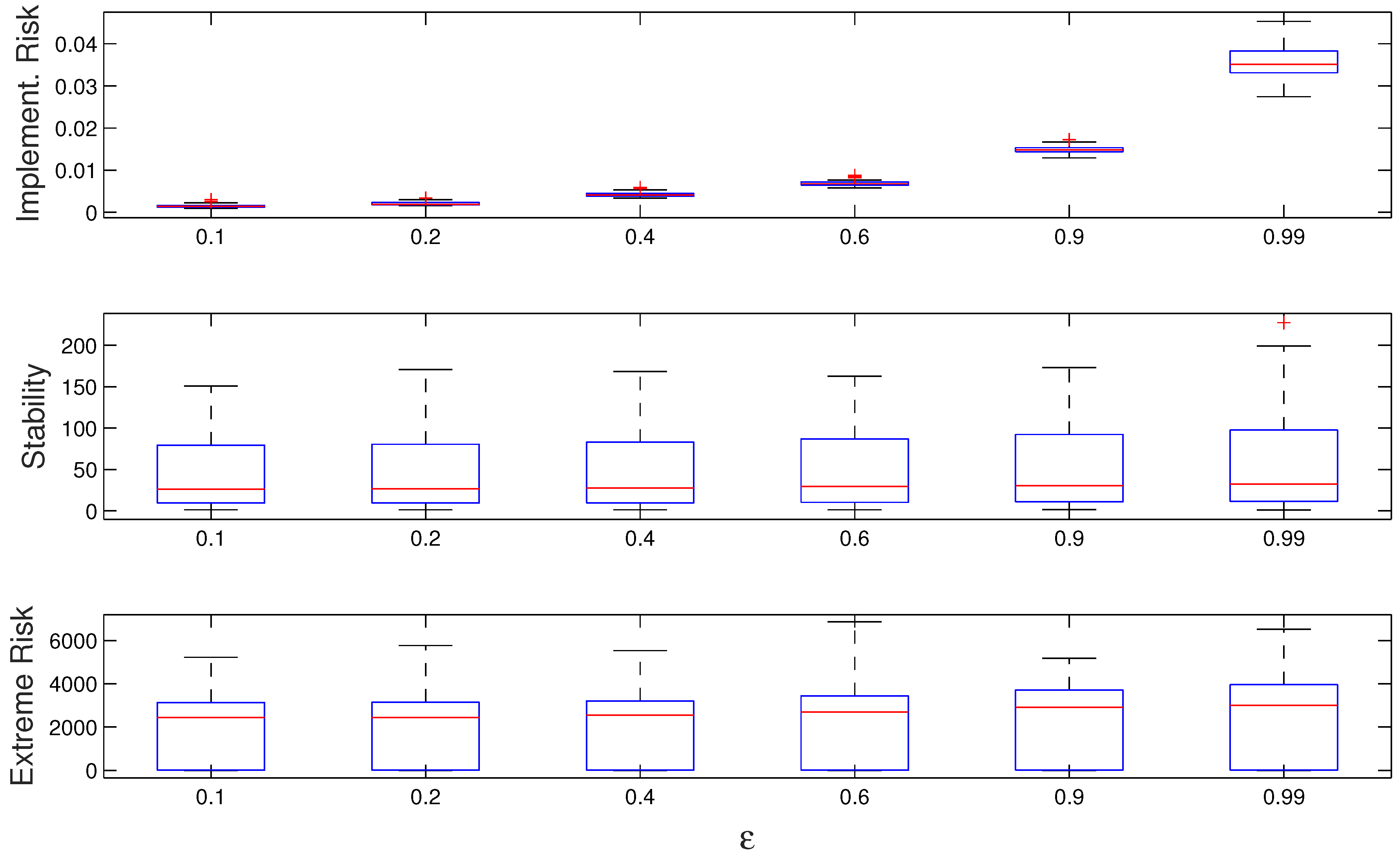
- Implementation Risk This metric estimates the robustness of a given portfolio structure taking into consideration the changes in risk and return due to deviations in an initially adopted investment strategy. The portfolio robustness is estimated based on the ratio between deviations in risk–return values and portfolio weights. This metric is calculated as shown in Equation (10). Smaller values of this metric correspond to more robust portfolios.
- Stability This metric measures the sensitivity of the portfolios included in the efficient frontier to a number of potential scenarios where asset returns and their variance–covariance matrix deviate from the expected values. The stability of a portfolio is measured by averaging the Mahalanobis distances between the expected pair of risk–return in the efficient frontier and the expected risk–return in S different scenarios. The metric is calculated as follows:where is the Mahalanobis distance between and , the risk and return for portfolio p in the period computed using the parameters for the scenario i. A set of 500 likely alternative scenarios is generated from historical data by using a nonparametric bootstrap. The higher the average dispersion, the less reliable the expected behavior of the current solution.
- Extreme Risk This metric evaluates the sensitivity of the solutions to worst-case scenarios. It is closely related to the measure of Stability. The difference is that, instead of considering the average for all S scenarios, a small subset is only taken into account. Specifically, the computation uses 1% of most problematic scenarios. These scenarios are identified by resampling historical returns 500 times, computing the average returns and the variance–covariance matrix for each of them, and including in the computation five scenarios for which the behavior of the portfolios in the solution differ more from the expected ones. The higher the metric, the higher the risk.
3. Results
The results in terms of the three performance metrics are summarized in Table 2. This table presents the mean and median values over the 60 scenarios and 20 runs per scenario for both the non-robust and the robust versions of the algorithm. The latter is studied with different values of the dispersion parameter . The presented results clearly show connection between the choice of the algorithm and the quality of the output. The robustness-based SMS-EMOA systematically provides better results than the base version with respect to the considered metrics.
The statistical significance of all the differences between the median values for the non-robust version of the algorithm versus the robust one was tested with the Mann–Whitney test, and they were significant at the 1% level.
As expected, the quality of obtained solutions with respect to robustness is highly related to the dispersion parameter. As the value of is decreased, the algorithm provides solutions with a higher robustness to both estimation and implementation risks measured by the corresponding metrics. It is an interesting observation, as the definition of a robustness measure used in the fitness assignment procedure only relies on the notion of implementation risk. The calculation of fitness does not explicitly involve a measure for estimation risk. This way, the experimental results suggest that there is some sort of connection between the two risks, as solutions more tolerant to implementation risk appear to be more tolerant to estimation risk as well. The advantage of the proposed approach lies in its ability to address both risks.
Given that experiments involved 60 optimization problems with 20 independent runs for each problem, Figure 1 illustrates, in the form of boxplots, the connection between the dispersion parameter and the distribution of the results regarding performance metrics. The presented plots show how the dispersion across metrics tends to grow for larger values of the parameter .
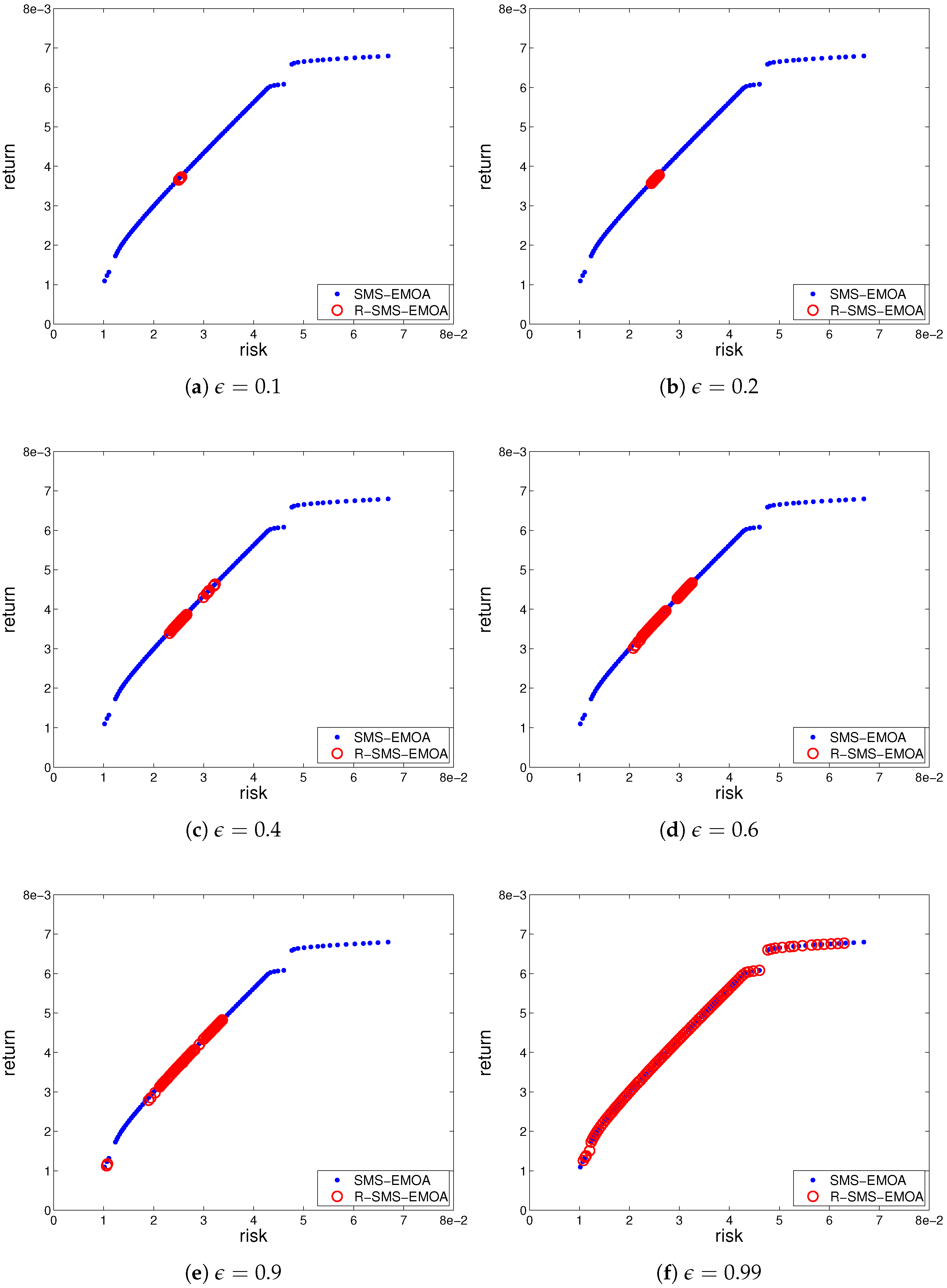
A better insight into the nature of the found solutions can be obtained by analyzing Figure 2. The plots presented in this figure show the efficient frontiers with the best value of the robustness metric over 20 runs, found by the algorithm for the optimization parameters derived from the first window. In these plots, the dots represent the solutions obtained by the non-robust algorithm. The peculiar structure of the upper-right section of the curve is due to the constraints considered in the problem. The circles show the solutions found by the robustness-based variant with different settings of the dispersion parameter . The influence of this parameter on the produced results can be easily observed.
4. Discussion
The algorithm converges to the efficient frontier, focusing on its specific regions. The focus is determined by the robustness of solutions. By setting , the user can express his/her preferences for robustness and obtain a set of solutions with desirable features. Increasing the value of leads to a larger extent of the efficient frontier covered by the population. On the other hand, for a small value of , the population converges to the most robust region of the efficient frontier. Such region exhibits a higher tolerance to deviations in asset allocations. Furthermore, we can observe that the robust regions do not need to be contiguous. This results demonstrate that, changing the parameter , the user can effectively focus the search on the regions with the preferred degree of robustness. This is a useful characteristic of the algorithm, as, in practice, not all solutions in the efficient frontier are relevant to the investor. If the investor is adverse to the risk in portfolio implementation, a low value of dispersion parameter can translate this preference. Alternatively, if the investor is indifferent to this type of risk, the value of can be increased. As the above results show, as a byproduct of managing robustness to implementation risk, we obtain solutions are also more robust with in terms estimation risk, which is a clear benefit for the investor.
It is also important to emphasize that a fine-grained approximation of the preferred portion of the efficient frontier is useful for decision making. This is particularly relevant to asset managers considering a large number of assets for investment. This is because apparently small differences between portfolios in the objective space would correspond to large distances in the decision space, i.e., differences between investment strategies.
The results make apparent another two interesting trends. On one hand, the portfolios that are more prone to implementation risk are on both extremes of the efficient frontier, especially on the high risk-high return area. On the other hand, we observe how the extension required to cover a small number of portfolios can have a sizable impact on the metrics. Figure 2f shows how a few extreme values cause the differences observed in Table 2. Such results are also consistent with much of professional practice. Asset allocations involving portfolios close to the extremes of the efficient frontier are rarely recommended, as investors find that either returns are too low, or they are too risky. As we can see, in addition to these problems, we can add higher implementation risk.
In terms of the convergence pattern for the algorithm, Figure 3 shows the evolution of the robustness to implementation risk as a function of the number of fitness evaluations for different values of . The data shows the average measure over 20 runs for the first time period. Larger tolerances to uncertainty regarding risk implementation require a more exhaustive search and, therefore, more evaluations. The improvement of the metric over time is quite dramatic. For lower values of , the indicator tends to stabilize around 3000 to 4000 fitness calls. When , the required number goes up to 6000–7000. This plot confirms the ability of the proposed fitness assignment procedure to continuously evolve the population with regard to robustness.
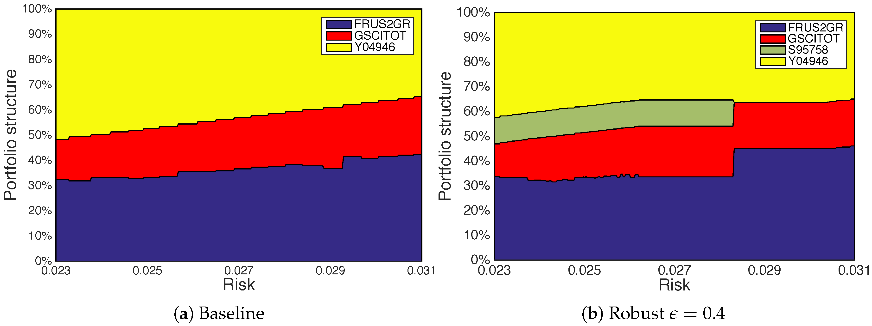
Finally, we look into an additional aspect, the structure of the found portfolios. Figure 4 presents the composition maps for the portfolios across different risk levels for the non-robust algorithm, Baseline, and the robust version with . More specifically, it represents the portfolios found for the first window, in the run already shown in Figure 2c. Instead of considering the whole range, we make the results more easily comparable focusing the attention on the central area between the lowest and the highest point in terms of risk where there is an overlap. Because the portfolios included in the solution are not evenly distributed and there is no perfect overlap in terms of risk, the comparison is performed based on the closest pairs of portfolios.
It can be seen that the portfolios offering the best returns for these levels of risk require only a fraction of the available investment alternatives. The non-robust strategy provides solutions relying only on three assets (the initial portfolio consists of 32.46% FRUS2GR, 17.45% GSCITOT and 51.72% Y04946). Conversely, the robust version includes a 10.56% investment in S95758 for the lowest risk level that remains at a similar point for most portfolios in the range. Although the composition map is presented for the robust version with , a similar general pattern is observed for other values of the dispersion parameter. The choice is justified by a balance of robustness and a number of overlapping portfolios that are significantly higher than for or .
These results show that more diversified portfolios are obtained when seeking robust solutions in mean-variance portfolio optimization. This observation is consistent with those reported in the financial literature. For instance, a similar pattern was observed in [41,42] when using a resampling technique to obtain portfolios tolerant to uncertainty related to future asset returns and variance–covariance matrix. The advantage of the proposed approach is that it enables the optimization to focus on robust and diverse portfolios, thereby providing a fine-grained approximation of the most preferred region.
We consider that there is no technical reason to think that suggested approach could not solve large-scale problems. However, the computational cost involved is likely be very high. Operators like the reconstruction one would probably have to be redesigned, as the algorithm is not developed for large-scale portfolio optimization and the implementation would also have to be optimized to be parallelized. Finally, working on these large-scale problems would also require considering additional steps. Among them, a key one would be the shrinkage of the variance–covariance matrix. Depending on sample size, the sample variance matrix is likely to be unsuitable, due to the estimation error, or singular. However, this problem has to do with the domain, no with the approach introduced here.
Finally, the method introduced in this paper might be successfully adapted to be used in other fields of application. We feel that the exploration of the applicability of the algorithm in domains like assembly line balancing [43]; design of energy supply systems [44]; compressed sensing [45,46] or support vector machines [47] are likely to be fruitful.
5. Conclusions
This paper proposed an approach to address the issue of robustness in a portfolio optimization. This approach extends a popular SMS-EMOA by incorporating the robustness measure into the fitness of population members. The degree to which the robustness influences the fitness is determined by the dispersion parameter. This parameter translates the user preferences for robustness and enables to direct the population towards the most preferred regions of the search space.
The experimental validation of the technique was performed through 60 asset allocation exercises for eight broad financial indexes that represent different asset classes, with a sample covering 15-years of market data. The results show that the portfolios obtained by the robustness-based approach are significantly more robust to estimation and portfolio implementation risks than those obtained by the standard algorithm. The obtained solutions are highly affected by the desirable degree of robustness specified before the search. The lower the value of the dispersion parameter, the higher the robustness of solutions. The structure of the robust portfolios differs from the non-robust ones. While they share the same basic composition, they tend to be more diversified. This feature of robust portfolios is considered very positive and is consistent with past findings regarding resampled portfolios designed to tolerate noisy optimization parameters. Thus, our findings show that the robustness-based SMS-EMOA is an effective tool for coping with uncertainties in portfolio optimization and can be used to support decision-making by providing the most relevant solutions with respect to the expressed preference information.
Among the remaining open questions that could make future extension of this work, we could mention scalability studies to evaluate and enhance the performance of the algorithm to a large number of investment alternatives. Others would be the implementation of parallel versions of the approach; a study of the sensitivity of results to the use of other evolutionary operators; or the hybridization with other strategies, like the fuzzy gravitational search algorithm, would also be an option [48].
Acknowledgments
Sandra Garcia-Rodriguez and David Quintana acknowledge financial support granted by the Spanish Ministry of Economy and Competitivity under grant ENE2014-56126-C2-2-R. Roman Denysiuk and Antonio Gaspar-Cunha were supported by the Portuguese Foundation for Science and Technology under grant PEst-C/CTM/LA0025/2013 (Projecto Estratégico-LA 25-2013-2014-Strategic Project-LA 25-2013-2014).
Author Contributions
David Quintana, Roman Denysiuk, Sandra Garcia-Rodriguez and Antonio Gaspar-Cunha conceived and designed the experiments; Roman Denysiuk and Sandra Garcia-Rodriguez performed the experiments; Roman Denysiuk and David Quintana analyzed the data; and David Quintana, Roman Denysiuk and Sandra Garcia-Rodriguez wrote the paper.
Conflicts of Interest
The authors declare no conflict of interest. The founding sponsors had no role in the design of the study; in the collection, analyses, or interpretation of data; in the writing of the manuscript, and in the decision to publish the results.
References
- Markowitz, H. Portfolio Selection. J. Financ. 1952, 7, 77–91. [Google Scholar]
- Markowitz, H. Portfolio Selection: Efficient Diversification of Investments; John Wiley & Son: New York, NY, USA, 1959. [Google Scholar]
- Daneshmand, A.; Facchinei, F.; Kungurtsev, V.; Scutari, G. Hybrid Random/Deterministic Parallel Algorithms for Nonconvex Big Data Optimization. IEEE Trans. Signal Process. 2014, 63, 3914–3929. [Google Scholar] [CrossRef]
- Pelusi, D.; Tivegna, M. Optimal trading rules at hourly frequency in the foreign exchange markets. In Mathematical and Statistical Methods for Actuarial Sciences and Finance; Perna, C., Sibillo, M., Eds.; Springer: Milan, Italy, 2012; pp. 341–348. [Google Scholar]
- Pelusi, D.; Tivegna, M.; Ippoliti, P. Improving the profitability of Technical Analysis through intelligent algorithms. J. Int. Math. 2013, 16, 203–215. [Google Scholar] [CrossRef]
- Pelusi, D.; Tivegna, M.; Ippoliti, P. Intelligent algorithms for trading the euro-dollar in the foreign exchange market. In Mathematical and Statistical Methods for Actuarial Sciences and Finance; Springer: Cham, Switzerland, 2014; pp. 243–252. [Google Scholar]
- Ponsich, A.; Jaimes, A.L.; Coello, C.A.C. A Survey on Multiobjective Evolutionary Algorithms for the Solution of the Portfolio Optimization Problem and Other Finance and Economics Applications. IEEE Trans. Evol. Comput. 2013, 17, 321–344. [Google Scholar] [CrossRef]
- Metaxiotis, K.; Liagkouras, K. Multiobjective Evolutionary Algorithms for Portfolio Management: A Comprehensive Literature Review. Expert Syst. Appl. 2012, 39, 11685–11698. [Google Scholar] [CrossRef]
- Lwin, K.; Qu, R.; Kendall, G. A learning-guided multi-objective evolutionary algorithm for constrained portfolio optimization. Appl. Soft Comput. 2014, 24, 757–772. [Google Scholar] [CrossRef]
- Yue, W.; Wang, Y.; Dai, C. An Evolutionary Algorithm for Multiobjective Fuzzy Portfolio Selection Models with Transaction Cost and Liquidity. Math. Probl. Eng. 2015, 2015. [Google Scholar] [CrossRef]
- Babaei, S.; Sepehri, M.M.; Babaei, E. Multi-objective portfolio optimization considering the dependence structure of asset returns. Eur. J. Oper. Res. 2015, 244, 525–539. [Google Scholar] [CrossRef]
- Liagkouras, K.; Metaxiotis, K. A new Probe Guided Mutation operator and its application for solving the cardinality constrained portfolio optimization problem. Expert Syst. Appl. 2014, 41, 6274–6290. [Google Scholar] [CrossRef]
- Fliege, J.; Werner, R. Robust multiobjective optimization and applications in portfolio optimization. Eur. J. Oper. Res. 2014, 234, 422–433. [Google Scholar] [CrossRef]
- Kim, W.C.; Kim, M.J.; Kim, J.H.; Fabozzi, F.J. Robust portfolios that do not tilt factor exposure. Eur. J. Oper. Res. 2014, 234, 411–421. [Google Scholar] [CrossRef]
- Beume, N.; Naujoks, B.; Emmerich, M. SMS-EMOA: Multiobjective Selection Based on Dominated Hypervolume. Eur. J. Oper. Res. 2007, 181, 1653–1669. [Google Scholar] [CrossRef]
- Ye, K.; Parpas, P.; Rustem, B. Robust portfolio optimization: A conic programming approach. Comput. Optim. Appl. 2012, 52, 463–481. [Google Scholar] [CrossRef]
- Toma, A.; Leoni-Aubin, S. Robust Portfolio Optimization Using Pseudodistances. PLoS ONE 2015, 10, e0140546. [Google Scholar] [CrossRef] [PubMed]
- Kilianová, S.; Trnovská, M. Robust portfolio optimization via solution to the Hamilton–Jacobi–Bellman equation. Int. J. Comput. Math. 2016, 93, 725–734. [Google Scholar] [CrossRef]
- Hassan, G.; Clack, C.D. Multiobjective Robustness for Portfolio Optimization in Volatile Environments. In Proceedings of the 10th Annual Conference on Genetic and Evolutionary Computation, Atlanta, GA, USA, 12–16 July 2008; ACM: New York, NY, USA, 2008; pp. 1507–1514. [Google Scholar]
- Sadjadi, S.J.; Gharakhani, M.; Safari, E. Robust optimization framework for cardinality constrained portfolio problem. Appl. Soft Comput. 2012, 12, 91–99. [Google Scholar] [CrossRef]
- Fastrich, B.; Winker, P. Robust portfolio optimization with a hybrid heuristic algorithm. Comput. Manag. Sci. 2012, 9, 63–88. [Google Scholar] [CrossRef]
- Lim, D.; Ong, Y.S.; Lim, M.H.; Jin, Y. Single/multi-objective inverse robust evolutionary design methodology in the presence of uncertainty. In Evolutionary Computation in Dynamic and Uncertain Environments; Springer: Berlin, Germany, 2007; pp. 437–456. [Google Scholar]
- Berutich, J.M.; Luna, F.; López, F. On the quest for robust technical trading strategies using multi-objective optimization. AI Commun. 2014, 27, 453–471. [Google Scholar]
- García, S.; Quintana, D.; Galván, I.M.; Isasi, P. Time-stamped resampling for robust evolutionary portfolio optimization. Expert Syst. Appl. 2012, 39, 10722–10730. [Google Scholar] [CrossRef] [Green Version]
- García-Rodríguez, S.; Quintana, D.; Galván, I.M.; Isasi, P. Multiobjective Algorithms with Resampling for Portfolio Optimization. Comput. Inf. 2013, 32, 777–796. [Google Scholar]
- García, S.; Quintana, D.; Galván, I.M.; Isasi, P. Extended Mean–variance Model for Reliable Evolutionary Portfolio Optimization. AI Commun. 2014, 27, 315–324. [Google Scholar]
- Azevedo, C.R.B.; Von Zuben, F.J. Anticipatory Stochastic Multi-Objective Optimization for Uncertainty Handling in Portfolio Selection. In Proceedings of the 2013 IEEE Congress on Evolutionary Computation, Fiesta Americana Grand Coral Beach Hotel, Cancun, Mexico, 20 June 2013; pp. 157–164. [Google Scholar]
- Deb, K.; Gupta, H. Introducing Robustness in Multi-Objective Optimization. Evol. Comput. 2006, 14, 463–494. [Google Scholar] [CrossRef] [PubMed]
- Jin, Y.; Sendhoff, B. Trade-Off between Performance and Robustness: An Evolutionary Multiobjective Approach. In Proceedings of the Evolutionary Multi-Criterion Optimization: Second International Conference, EMO 2003, Faro, Portugal, 8–11 April 2003; Fonseca, C.M., Fleming, P.J., Zitzler, E., Thiele, L., Deb, K., Eds.; Springer: Berlin/Heidelberg, Gemany, 2003; pp. 237–251. [Google Scholar]
- Gaspar-Cunha, A.; Covas, J.A. Robustness in multi-objective optimization using evolutionary algorithms. Comput. Optim. Appl. 2008, 39, 75–96. [Google Scholar] [CrossRef]
- Gaspar-Cunha, A.; Ferreira, J.; Recio, G. Evolutionary Robustness Analysis for Multi-Objective Optimisation: Benchmark Problems. Struct. Multidiscip. Optim. 2014, 49, 771–793. [Google Scholar] [CrossRef]
- Deb, K.; Gupta, S.; Daum, D.; Branke, J.; Mall, A.; Padmanabhan, D. Reliability-Based Optimization Using Evolutionary Algorithms. IEEE Trans. Evol. Comput. 2009, 13, 1054–1074. [Google Scholar] [CrossRef]
- Beyer, H.G.; Sendhoff, B. Robust optimization—A comprehensive survey. Comput. Methods Appl. Mech. Eng. 2007, 196, 3190–3218. [Google Scholar] [CrossRef]
- Jin, Y.; Branke, J. Evolutionary optimization in uncertain environments—A survey. IEEE Trans. Evol. Comput. 2005, 9, 303–317. [Google Scholar] [CrossRef]
- Azevedo, C.R.B.; Von Zuben, F.J. Regularized hypervolume selection for robust portfolio optimization in dynamic environments. In Proceedings of the 2013 IEEE Congress on Evolutionary Computation, Cancun, Mexico, 20–23 June 2013; pp. 2146–2153. [Google Scholar]
- Deb, K.; Agrawal, R.B. Simulated Binary Crossover for Continuous Search Space. Complex Syst. 1995, 9, 115–148. [Google Scholar]
- Deb, K. Multi-Objective Optimization Using Evolutionary Algorithms; John Wiley & Sons, Inc.: New York, NY, USA, 2001. [Google Scholar]
- Deb, K.; Pratap, A.; Agarwal, S.; Meyarivan, T. A Fast and Elitist Multiobjective Genetic Algorithm: NSGA-II. IEEE Trans. Evol. Comput. 2002, 6, 182–197. [Google Scholar] [CrossRef]
- Zitzler, E.; Thiele, L. Multiobjective Optimization Using Evolutionary Algorithms—A Comparative Case Study. In Proceedings of the Conference on Parallel Problem Solving From Nature, Ruhr, Germany, 1–3 October 1990; pp. 292–304. [Google Scholar]
- Zitzler, E.; Thiele, L. An Evolutionary Algorithm for Multiobjective Optimization: The Strength Pareto Approach; Institut für Technische Informatik und Kommunikationsnetze (TIK): Zurich, Switzerland, 1998. [Google Scholar]
- Idzorek, T.M. Developing Robust Asset Allocations; Technical Report; Ibbotson Associates: Chicago, IL, USA, 2006. [Google Scholar]
- Michaud, R.; Michaud, R. Estimation error and portfolio optimization: A resampling solution. J. Invest. Manag. 2008, 6, 8–28. [Google Scholar] [CrossRef]
- Chica, M.; Bautista, J.; Damas, S.; Cordon, O. Adaptive IDEA for Robust Multiobjective Optimization, Application to the r-TSALBP-m/A. In Proceedings of the 2015 IEEE Symposium Series on Computational Intelligence, Cape Town, South Africa, 7–10 December 2015; pp. 1013–1020. [Google Scholar]
- Majewski, D.E.; Wirtz, M.; Lampe, M.; Bardow, A. Robust multi-objective optimization for sustainable design of distributed energy supply systems. Comput. Chem. Eng. 2017, 102, 26–39. [Google Scholar] [CrossRef]
- Dassios, I.K.; Fountoulakis, K.; Gondzio, J. A Preconditioner for A Primal-Dual Newton Conjugate Gradient Method for Compressed Sensing Problems. SIAM J. Sci. Comput. 2015, 37, A2783–A2812. [Google Scholar] [CrossRef]
- Dassios, I.; Fountoulakis, K.; Gondzio, J. A Second-Order Method for Compressed Sensing Problems with Coherent and Redundant Dictionaries. arXiv 2014, arXiv:1405.4146. [Google Scholar]
- Ni, T.; Zhai, J. A Matrix-free Smoothing Algorithm for Large-scale Support Vector Machines. Inf. Sci. 2016, 358, 29–43. [Google Scholar] [CrossRef]
- Pelusi, D.; Mascella, R.; Tallini, L. Revised Gravitational Search Algorithms Based on Evolutionary-Fuzzy Systems. Algorithms 2017, 10, 44. [Google Scholar] [CrossRef]
Figure 1.
Influence of the dispersion parameter on the distribution of robustness metrics. Boxplots depict the quartile distribution of robustness for the sets of experiments.
Figure 1.
Influence of the dispersion parameter on the distribution of robustness metrics. Boxplots depict the quartile distribution of robustness for the sets of experiments.

Figure 2.
Influence of the dispersion parameter on the size of the robust region in portfolio selection.
Figure 2.
Influence of the dispersion parameter on the size of the robust region in portfolio selection.

Figure 3.
Evolution of the robustness metric over the number of function evaluations. The plot refers to the mean values over 20 runs.
Figure 3.
Evolution of the robustness metric over the number of function evaluations. The plot refers to the mean values over 20 runs.

Figure 4.
Composition of the best portfolios identified by the standard algorithm and the robustness-based one for the overlapping range of risks.
Figure 4.
Composition of the best portfolios identified by the standard algorithm and the robustness-based one for the overlapping range of risks.


Table 1.
Indices used in the experimental work. S&P GSCI Commodity Total Return is the Standard & Poor’s former Goldman Sachs Commodity Index and MSCI EAFE is the Morgan Stanley Capital International large and mid-cap securities index for Europe, Australasia and Far East.
Table 1.
Indices used in the experimental work. S&P GSCI Commodity Total Return is the Standard & Poor’s former Goldman Sachs Commodity Index and MSCI EAFE is the Morgan Stanley Capital International large and mid-cap securities index for Europe, Australasia and Far East.
| Name | Code |
|---|---|
| Frank Russell 1000 Growth | FRUS1GR |
| Frank Russell 1000 Value | FRUS1VA |
| Frank Russell 2000 Growth | FRUS2GR |
| Frank Russell 2000 Value | FRUS2VA |
| S&P GSCI Commodity Total Return | GSCITOT |
| MSCI EAFE | MSEAFEL |
| Barclays Corporate Intermediate | S95758 |
| Barclays Intermediate US GVT/CREDIT | Y04946 |
Table 2.
Results for baseline and robustness-based S-metric selection evolutionary multiobjective optimization algorithms (SMS-EMOA). Differences in percentage vs. standard version.
Table 2.
Results for baseline and robustness-based S-metric selection evolutionary multiobjective optimization algorithms (SMS-EMOA). Differences in percentage vs. standard version.
| SMS-EMOA | Implem. Risk | Stability | Extr. Risk | |||||
|---|---|---|---|---|---|---|---|---|
| Version | Mean | Diff. (%) | Mean | Diff. (%) | Mean | Diff. (%) | ||
| Mean | Standard | 0.0770 | 68.56 | 2984.71 | ||||
| Robust | 0.99 | 0.0356 | −53.8% | 53.44 | −22.0% | 2289.04 | −23.3% | |
| 0.9 | 0.0148 | −80.7% | 50.14 | −26.9% | 2124.96 | −28.8% | ||
| 0.6 | 0.0069 | −91.1% | 47.55 | −30.6% | 1996.60 | −33.1% | ||
| 0.4 | 0.0043 | −94.5% | 45.07 | −34.3% | 1862.10 | −37.6% | ||
| 0.2 | 0.0021 | −97.3% | 43.77 | −36.2% | 1788.66 | −40.1% | ||
| 0.1 | 0.0015 | −98.0% | 43.40 | −36.7% | 1769.18 | −40.7% | ||
| Median | Standard | 0.0769 | 39.30 | 4276.12 | ||||
| Robust | 0.99 | 0.0327 | −57.5% | 32.25 | −17.9% | 3000.91 | −29.8% | |
| 0.9 | 0.0144 | −81.3% | 30.40 | −22.6% | 2918.74 | −31.7% | ||
| 0.6 | 0.0062 | −92.0% | 29.29 | −25.5% | 2705.15 | −36.7% | ||
| 0.4 | 0.0036 | −95.4% | 27.27 | −30.6% | 2550.84 | −40.3% | ||
| 0.2 | 0.0016 | −97.9% | 26.39 | −32.8% | 2448.58 | −42.7% | ||
| 0.1 | 0.0010 | −98.7% | 26.12 | −33.5% | 2442.56 | −42.9% | ||
© 2017 by the authors. Licensee MDPI, Basel, Switzerland. This article is an open access article distributed under the terms and conditions of the Creative Commons Attribution (CC BY) license (http://creativecommons.org/licenses/by/4.0/).
Share and Cite
MDPI and ACS Style
Quintana, D.; Denysiuk, R.; Garcia-Rodriguez, S.; Gaspar-Cunha, A. Portfolio Implementation Risk Management Using Evolutionary Multiobjective Optimization. Appl. Sci. 2017, 7, 1079. https://0-doi-org.brum.beds.ac.uk/10.3390/app7101079
AMA Style
Quintana D, Denysiuk R, Garcia-Rodriguez S, Gaspar-Cunha A. Portfolio Implementation Risk Management Using Evolutionary Multiobjective Optimization. Applied Sciences. 2017; 7(10):1079. https://0-doi-org.brum.beds.ac.uk/10.3390/app7101079
Chicago/Turabian StyleQuintana, David, Roman Denysiuk, Sandra Garcia-Rodriguez, and António Gaspar-Cunha. 2017. "Portfolio Implementation Risk Management Using Evolutionary Multiobjective Optimization" Applied Sciences 7, no. 10: 1079. https://0-doi-org.brum.beds.ac.uk/10.3390/app7101079
Note that from the first issue of 2016, this journal uses article numbers instead of page numbers. See further details here.