Determination of the Constants of GTN Damage Model Using Experiment, Polynomial Regression and Kriging Methods

Abstract

Damage models, particularly the Gurson–Tvergaard–Needleman (GTN) model, are widely used in numerical simulation of material deformations. Each damage model has some constants which must be identified for each material. The direct identification methods are costly and time consuming. In the current work, a combination of experimental, numerical simulation and optimization were used to determine the constants. Quasi-static and dynamic tests were carried out on notched specimens. The experimental profiles of the specimens were used to determine the constants. The constants of GTN damage model were identified through the proposed method and using the results of quasi-static tests. Numerical simulation of the dynamic test was performed utilizing the constants obtained from quasi-static experiments. The results showed a high precision in predicting the specimen’s profile in the dynamic testing. The sensitivity analysis was performed on the constants of GTN model to validate the proposed method. Finally, the experiments were simulated using the Johnson–Cook (J–C) damage model and the results were compared to those obtained from GTN damage model.

1. Introduction

Today, the finite element codes have substituted expensive and tedious experiments for mechanical characterization of materials. The accuracy of material damage and material models plays an important role in the performance of the codes. All models involve a number of constants which must normally be determined by experiment. The accuracy of the models obviously depends on the accuracy of the constants.

1.1. Damage Models

Various damage models can be found in the literature. Some of the most important models are briefly described in this section.

1.1.1. Gurson–Tvergaard–Needleman Model

Gurson, Tvergaard and Needleman’s damage model (GTN model) [1] is an analytical model that predicts ductile fracture on the basis of nucleation, growth and coalescence of voids in materials. The model is defined as:

$$\varphi =\frac{{\sigma }_e^2}{{\sigma }_M^2}+2q_1{f}^{\ast }\cosh \left[\frac{tr\sigma }{2{\sigma }_M}\right]-1-{\left(q_1{f}^{\ast }\right)}^2=0$$

(1)

In which $q_1$ is the material constant, $tr\sigma$ is the sum of principal stresses, ${\sigma }_M$ is the equivalent flow stress and f* is the ratio of voids effective volume to the material volume ratio defined as follows:

$$f^{\ast }\left(f\right)=f_{c}iff\le f_c,$$

(2)

$$f^{\ast }\left(f\right)=f_c+\frac{(1/q_1)-f_c}{f_f-f_c}\left(f-f_c\right)iff>f_c,$$

(3)

where f is the voids’ volume ratio, f_c is the voids’ volume ratio at the beginning of nucleation and f_f is the voids’ volume ratio when fracture occurs. The equivalent flow stress (${\sigma }_M$) is obtained from the following work hardening relation:

$${\sigma }_M\left({\epsilon }_M^{pl}\right)={\sigma }_y{\left(\frac{{\epsilon }_M^{pl}}{{\epsilon }_y}+1\right)}^n,$$

(4)

In which n is the strain-hardening exponent and ${\epsilon }_M^{pl}$ is the equivalent plastic strain. The voids’ growth rate is the sum of existing voids growth ${\dot{f}}_g$ and the new voids’ nucleation ${\dot{f}}_n$.

$$\dot{f}={\dot{f}}_n+{\dot{f}}_g,$$

(5)

where the components are further formulated as follows:

$${\dot{f}}_g=\left(1-f\right)tr{\dot{\epsilon }}^{pl},$$

(6)

$${\dot{f}}_n=A{\dot{\epsilon }}_M^{pl},$$

(7)

$$A=\frac{f_n}{S_n\sqrt{2\pi }}\exp \left[-\frac{1}{2}\left(\frac{{\epsilon }_M^{pl}-{\epsilon }_N}{s_N}\right)\right],$$

(8)

In which $tr{\dot{\epsilon }}^{pl}=\left({\dot{\epsilon }}_x+{\dot{\epsilon }}_y+{\dot{\epsilon }}_z\right)$ is the volume plastic strain rate, $s_N$ is the voids’ nucleation mean quantity, f_n is volume ratio of the second phase particles (responsible for the voids’ nucleation) and ${\epsilon }_N$ is mean strain at the time of voids’ nucleation. So, GTN model involves ten parameters which can be defined in a vector form by:

$$\varphi =\varphi \left({\sigma }_y{\epsilon }_{y}n{q}_1{f}_0{f}_c{f}_f{f}_n{\epsilon }_N{S}_N\right)$$

In this model, the effect of hydrostatic pressure on the voids’ growth is considered and the shear stress effect is ignored which in general cases makes the results questionable. Thus, although, this model can perfectly predict damage in tensile stress, it is not as accurate in shear stress tests. To overcome this shortcoming, an extension of the Gurson model was proposed by Nahshon and Hutchinson [2] that incorporates damage growth under low triaxial straining for shear-dominated states. Var et al. [3] identified material parameters for Gurson-type and Lemaitre-type constitutive models for low alloy steel based on a hybrid global–local optimization technique. Chang-Kyun et al. [4] used experiment and FE simulations for smooth and notched tensile bars, to calibrate the parameters in the GTN model. Malcher et al. [5] undertook a numerical comparative study based on GTN original model and two recent enhancements that included shear mechanisms, employing mathematical and numerical strategies to calibrate the material parameters.

1.1.2. Johnson–Cook Damage Model

Johnson and Cook [6] developed the following relation for failure strain:

$${\epsilon }_f=\left(D_1+D_2\exp \left(D_3\left(\frac{p}{{\sigma }_y}\right)\right)\right)\left(1+D_{4}Ln\dot{\epsilon }\right)\left(1+D_5{T}^{\ast }\right),$$

(9)

In which ${\epsilon }_f$ is the strain failure, $\frac{p}{{\sigma }_y}$ is the stress triaxiality parameter, $\dot{\epsilon }$ is strain rate and $T^{\ast }$ is the dimensionless temperature calculated by Equation (10). D₁ to D₅ are material constants.

$$T^{\ast }=\frac{T-T_{room}}{T_{melt}-T_{room}},$$

(10)

where T_room is the room temperature and T_melt is the material melting point. In the Johnson–Cook model, parameter D defined by Equation (11), represents the voids’ growth and is used as the fracture criterion.

$$D={\displaystyle \sum \frac{\Delta \epsilon }{{\epsilon }_f}},$$

(11)

This parameter is generally a function of strain rate and the stress triaxiality parameter. In this relation D is the damage coefficient and ∆ε is the plastic strain increment in each iteration. In the finite element numerical simulation the value D is calculated in every loading increment for each element. When the value of D reaches unity in an element, D = 1, fracture occurs in that element and the element is eliminated from the computations.

1.1.3. Rice and Tracey Model

Rice and Tracey [7] developed a mathematical model that relates to the voids’ growth to stress triaxiality parameter. In this model, voids’ growth rate is defined as follows:

$$\frac{dR}{R}=\alpha \exp \left(\frac{3}{2}\xi \right)d{\epsilon }^{pl},$$

(12)

In which $\alpha$ is the material constant and $\xi =\frac{{\sigma }_m}{{\sigma }_{eq}}$ is the stress triaxiality parameter. For considering the work hardening in Rice and Tracey model, Bermin [7] suggested the use of flow stress instead of yield stress in Equation (12). By integrating Equation (12) we can obtain:

$$Ln\frac{R}{R_0}={\displaystyle \int \alpha \exp \left(\frac{3}{2}\frac{{\sigma }_m}{{\sigma }_{eq}}\right)}d{\epsilon }^{pl},$$

(13)

1.1.4. Gunawardana Model

Gunawardena [8] developed a damage model on the basis of Rice and Tracey model. Assuming spherical growth of voids and rigid-plastic behavior of materials, the fracture reference strain ${\epsilon }_f$ is calculated for different states of stress triaxiality as follows:

$${\epsilon }_f={\epsilon }_0\exp \left(\frac{1}{2}-\frac{3}{2}\frac{{\sigma }_h}{{\sigma }_{eq}}\right),$$

(14)

In which ${\sigma }_h$ is the hydrostatic stress component. For this model D is the damage parameter for which the growth rate is defined as follows:

$$d\text{}D=\frac{d{\epsilon }_p}{{\epsilon }_f},$$

(15)

Integrating Equation (15) and using Equation (14) we obtain:

$$D=\frac{1}{{\epsilon }_0}{\displaystyle \underset{0}{\overset{{\epsilon }_p^c}{\int }}\exp \left(\frac{3}{2}\frac{{\sigma }_h}{{\sigma }_{eq}}-\frac{1}{2}\right)}d{\epsilon }_p,$$

(16)

Note that ${\epsilon }_p^c$ is the plastic strain in each increment of loading in which D is calculated. Damage occurs when the D parameter reaches unity. The most important advantage of this model is that it requires only constant (ε₀) to be determined.

1.2. The Constants Identification Methods

There are two methods which are generally used to determine the constants of damage model.

1.2.1. Metallography Method

Since damage models describe micromechanical processes, some of their constants can be obtained by metallographic methods. In this method, quantitative photography process is used for analyzing fractured surface metallography. Quantitative photography is a method for acquiring quantitative data from photos using special software designed for such purposes.

1.2.2. Numerical Methods

In this method, the computations continue until some geometrical parameters such as the final profile of the specimen predicted by numerical simulation converges to that obtained from an experiment such as tensile test. Plain or notched specimens can be used in the experiments.

Determination of the constants of Gurson damage model through direct measurement and experimental testing is very difficult. On the other hand, the response of materials in numerical simulation definitely depends on these constants. Consequently, the constants can be determined by comparing material response in different loading states in numerical simulation with that of experimental measurements.

Various researchers utilized this idea to find the damage models constants. Majzoobi et al. [9,10] obtained the variation of fracture strain versus stress triaxiality coefficient for notched steel and copper specimens of different notch radii. The results were used for determining the constants D₁ to D₃ in Johnson–Cook damage model. They also obtained the variation of fracture strain versus Ln $\dot{\epsilon }$ under dynamic test conditions. The results were employed for determining the constant D₄ in Johnson–Cook damage model.

Ochewit et al. [11] performed plain specimen tensile test and measured the fracture displacement of the specimen. Then, they simulated the same tests using a finite element code. The constants q₁, S_n, ε_n, f₀ and f_n were obtained from the literature. For determining f_c and f_f, simulation was performed for different sets of f_c and f_f and for each simulation the fracture displacement was recorded. The next step was to define the difference between fracture displacement of the specimens obtained from experiment and that of simulation as an objective function. By minimizing this objective function, f_c and f_f were identified. They used the computed constants for numerical simulation of automobile component under crash loading and found a good compatibility with experimental results.

In another study, Markus Feucht et al. [12] predicted the f_c and f_f constants of Gurson model for aluminum die cast alloy and high strength steel, using minimization of the difference between component displacement parameter obtained from numerical simulation and the one measured in tensile test of the plain sample. They applied the same constants in a numerical simulation of the tensile test of notched samples. Moreover, they used these constants for automobile components in crash tests. The results obtained were found to agree well with the experimental results.

Springmann and Kuna [13] determined the constants of Gurson damage model using the displacement-load curves obtained from experiment and a nonlinear optimization method. They defined the difference between the load measured in experiment and predicted by simulation at some points of displacement-load diagram as objective function for optimization. This objective function is defined as:

$$\varphi \left(p\right)=\frac{1}{2}{{\displaystyle \sum _{i=1}^{n_l}\left[f_i\left(p\right)-{\overline{f}}_i\left(p\right)\right]}}^2,$$

(17)

where, n_i is the number of points on displacement-load diagram, ϕ(p) is the objective function, $f_i\left(p\right)$ is the force obtained from simulation and ${\overline{f}}_i\left(p\right)$ is the force measured from experiment. The optimization of this objective function was accomplished by an iterative nonlinear method.

Broggiato et al. [14] used digital photography method for obtaining the specimen’s profile in each loading increment. By collecting the profiles for each loading increment, they acquired the data to determine the damage and material models constants. Kuna and Springmann [15] employed local deformation measurements to determine GTN damage model constants. At the beginning, they performed a simple tensile test on a notched specimen and obtained displacement for some specified points in each loading increment via displacement filed optical measurement technique. For the next step, they simulated their experiment numerically and obtained the displacement of a specified point for different values of damage model constants. Then, by defining the objective function Equation (18) and minimizing it with respect to damage model constants p, the optimized values of the constants were determined.

$$\varphi \left(p\right)=\frac{1}{2}{{\displaystyle \sum _{i=1}^{n_l}{\displaystyle \sum _{j=1}^{n_m}{\displaystyle \sum _{k=1}^3\left[{\left(u_k\left(p\right)\right)}_{ij}-{\left(u_k\right)}_{ij}\right]}}}}^2,$$

(18)

where, ϕ(p) is the objective function, n_l is the number of loading steps, n_m is the number of points specified, u_k (p) is the displacement calculated by simulation and u_k is the displacement obtained from experiment.

2. Materials and Methods

2.1. Experiments

The geometries of plain and notched specimens are illustrated in Figure 1. The specimens were fabricated according to ASTM standard from structural steel ST37. The quasi-static tests were carried out using Instron tensile testing machine.

The engineering and true stress-strain curves obtained from plain specimen test are illustrated in Figure 2. From the figure, the yield and ultimate stresses were obtained as:

$${\sigma }_y=400\mathrm{Mpa}{\sigma }_u=600\mathrm{Mpa}$$

Dynamic tests were performed using Flying Wage testing apparatus (a high rate testing device) [16,17]. A general view of the device is shown in Figure 3.

Figure 4 illustrates the sketch of the specimens used for dynamic tests.

The geometry of the notched specimen was measured precisely by the method of optical measurement before and after the test. The optical precise measurement machine utilizes a projector to project the magnified picture of the specimen on a white screen and measurements are made on this screen. Figure 5 illustrates the specimen picture projected on the measurement machine screen.

From the projected picture of the specimen, the change in the gauge length, ($\Delta L(\mathrm{mm})$) and the notch root diameter, ($\Delta d(\mathrm{mm})$), of the specimen are measured. The results are given in

Table 1. Quasi-static and dynamic measurements.

Test Type	Δd (mm)	ΔL (mm)
Quasi-static	1.675	1.95
Dynamic	1.36	1.57

for quasi and dynamic tests.

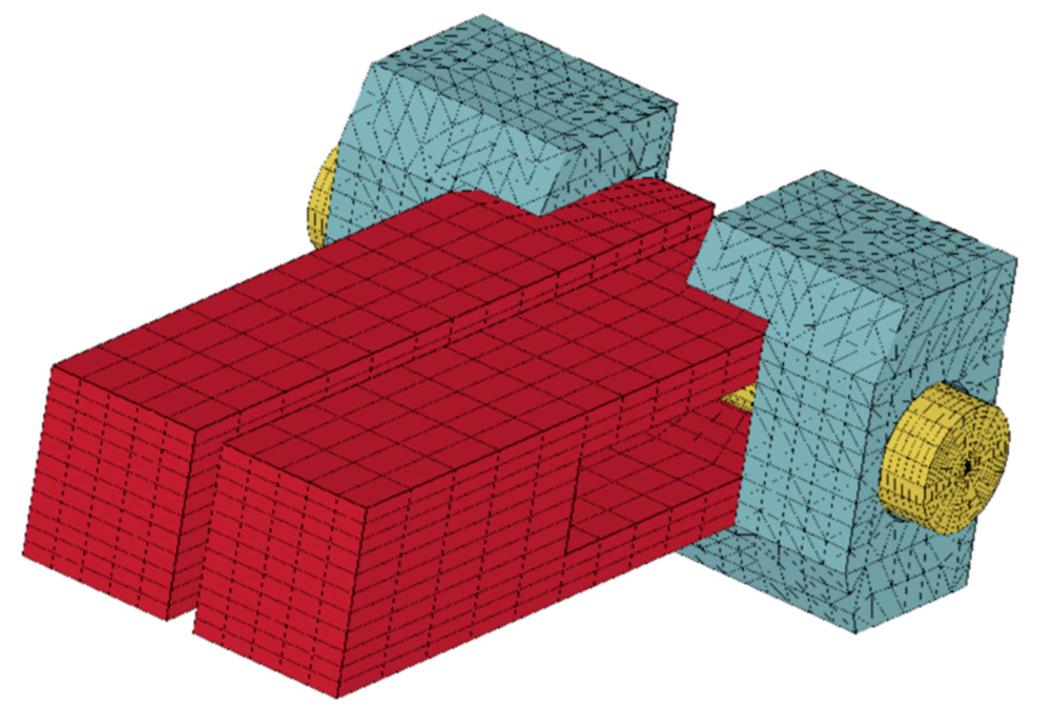
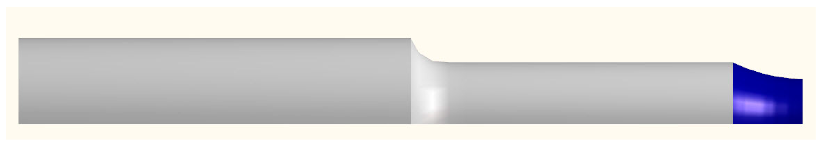
2.2. Numerical Simulations

2.2.1. Simulation of Quasi-Static Tests

As the plastic deformation accumulates only in the notch area, only this area is considered in numerical simulation of quasi-static test. Due to axisymmetric conditions of the specimens, only 1/4 of the specimen is simulated. Figure 6 illustrates the finite element model of the specimen.

2.2.2. Simulation of Dynamic Tests

As stated above, the dynamic tests were conducted on the “Flying wedge” testing apparatus. Therefore, the major parts of the Flying Wedge involved in pulling the specimen were considered in the finite element model of the dynamic test simulations. The simulations were performed using the hydrocode, Ls-dyna. Figure 7 and Figure 8 illustrate views of the 3-D and the finite element model of the wedge respectively. The model consists of the notched specimen, two sliders in which the specimen is mounted and the wedge plate. The plate impacts on the sliders and makes them move away from each other resulting in tension in the specimen. The strain rate can be varied by changing the impact velocity of the wedge plate. The dimensions and the boundary conditions of the model are exactly the same as those in the testing apparatus.

Figure 9 and Figure 10 illustrate the 3-D model and the finite element model of the dynamic testing specimen. As noted before, the damage phenomenon is highly dependent on plastic deformation. Again, as plastic deformation occurs only in notch area, a GTN model was used only for the simulation of this area. Therefore, a higher mesh density was considered in the notch area. The other parts of the specimen were modeled using a coarser mesh and were analyzed using elastic behavior for the material.

2.3. Identification of the Constants of GTN Model

2.3.1. Definition of the Objective Function

For determining the constants of GTN damage model a combination of experimental, numerical, and optimization methods were employed. This approach has already been used by Majzoobi et al. [18,19] for determining the constants of few material models. Of course, the optimization methods used by Majzoobi et al. are different from those used in this study. The elongation and fracture strain of the specimen were the most important design parameters used in this study. The fracture strain was computed as follows:

$${\epsilon }_f=2Ln\frac{d_0}{d_f}$$

(19)

In which d₀ is the initial diameter and d_f is the diameter after fracture. The constants of the damage model were determined in a way that the results of the numerical simulation for elongation and diameter reduction of the specimen after fracture have minimum deviation from the measurements of the experiment.

Thus, the difference between the numerical predictions and the experimental measurements for these two parameters was defined as the objective function. It is worth noting that if more parameters from tensile and shear tests are simultaneously considered in defining the optimization objective function, the optimized constants will be more accurate.

For defining the objective function in optimization the following parameters were used.

$$\Delta l_{experimental}={\overline{L}}_f-L_i,\hspace{1em}\Delta d_{experimental}={\overline{d}}_f-d_i,$$

(20a)

$$\Delta l_{numerical}=L_f\left(p\right)-L_i,\hspace{1em}\Delta d_{numerical}=d_f\left(p\right)-d_i,$$

(20b)

$$OB{J}^1=\Delta l_{experimental}-\Delta l_{numerical},$$

(20c)

$$OB{J}^2=\Delta d_{experimental}-\Delta d_{numerical},$$

(20d)

$$OBJ=\frac{OB{J}^1+OB{J}^2}{2},$$

(20e)

where, $L_i$ and $d_i$ are the initial length and diameter of the specimen before loading.

${\overline{L}}_f$ and ${\overline{d}}_f$ are the experimental length and diameter of the specimen after failure.

$L_f\left(p\right)$ and $d_f\left(p\right)$ are the numerical length and diameter of the specimen after failure.

$\Delta l_{experimental}$ is the experimental notch length change.

$\Delta l_{numerical}$ is the numerical notch length change.

$\Delta d_{experimental}$ is the measured notch root diameter of the specimen

$\Delta d_{numerical}$ is the numerical notch root diameter of the specimen

OBJ is the Objective function.

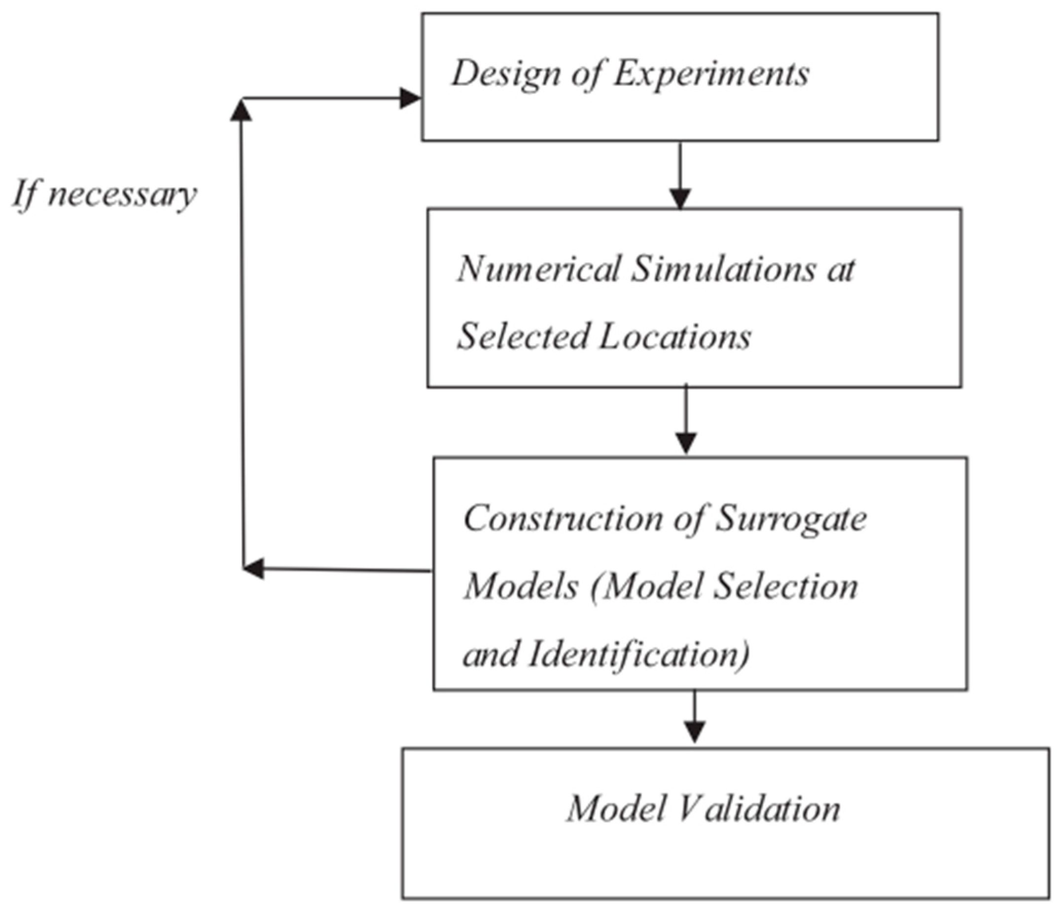
2.3.2. Surrogate-Based Optimization Method

An effective and efficient method to have cheap approximations of expensive black-box functions is the surrogate-based algorithm [20,21]. It is simply a numerical approximation of how an entity varies when the entities that affect it are varied. This method has also been widely employed to evaluate the numerical predictions which are calculated by expensive codes such as computational fluid dynamics (CFD) and nonlinear finite element method (NFEM) to speed up the analyzing process [22,23,24]. For implementing the surrogate-based optimization technique in a numerical simulation, the following steps should be taken [24,25]:

• Selecting the initial sampling points with a design of experiments (DoE) technique
• Performing the computationally expensive FE simulation for the selected points
• Fitting the surrogate model
• Optimizing the surrogate model and finding the new set of samples and
• Repeating steps 2–4 to reach convergence.

Figure 11 illustrates the flow chart of the surrogate-based optimization process.

In surrogate-based optimization there are different methods for generation of the surrogate function. This paper employs two methods of polynomial regression and Kriging. Each method is described briefly and the results obtained from the two methods applied for optimization are compared.

2.3.3. Design of Experiments (DOE)

The design of experiment defines how initial points in the variable space are selected. The evaluation process of the satisfactory coverage in the domain space and also the number of samples limitations due to computational expenses are two important elements for this step. There is a variety of DoE methods which can be found in the literature [24,25,26]. In this investigation Latin hypercube sampling (LHS) method [26,27] was adopted as the DoE method due to its good ability of filling domain space. A schematic of six sample points selection using LHS method for two variables is shown in Figure 12.

For the generation of a polynomial regression function having four constants, 15 initial samples were needed for which LHS design function of MATLAB (Vesion: 2017a, Company: MathWorks, City: Torino 10122, Country: Italy)code was applied. The same initial samples were also used for generation of Kriging function. In addition, five different trial sets of samples with 6, 7, 8, 9 and 10 samples were used for generation of Kriging function using LHS design function.

2.3.4. Polynomial Regression Method

In this method, the objective function is approximated by a polynomial of second order as below [28]:

$$OBJ\left(x\right)\cong a_0+{\displaystyle \sum _{i=1}^n{a}_i{x}_i}+{\displaystyle \sum _{i,j=1}^n{b}_{ij}{x}_i{x}_j},$$

(21)

In which, n is the number of constants of GTN damage model, and a₀, a_i and b_ij are the polynomial coefficients. The GTN model has 10 constants $\left({\sigma }_y{\epsilon }_{y}n{q}_1{f}_0{f}_c{f}_f{f}_N{\epsilon }_N{S}_N\right)$. σ_y, ε_y and n are obtained from stress-strain curve of plain specimen obtained from quasi-static tensile test. The optimum quantities of q₁ = 1.5, S_N = 0.1 and ε_N = 0.3 are taken from literature [29,30,31,32]. Therefore, four constants remain to be determined for structural steel ST37. The polynomial of second order for four variables has 15 coefficients as follows:

$$\begin{gathered} OBJ=a_0+a_1{x}_1+a_2{x}_2+a_3{x}_3+a_4{x}_4+a_5{x}_1^2+a_6{x}_2^2+a_7{x}_3^2+a_8{x}_4^2+a_9{x}_1{x}_2+ \\ {a}_{10}{x}_1{x}_3+a_{11}{x}_1{x}_4+a_{12}{x}_2{x}_3+a_{13}{x}_2{x}_4+a_{14}{x}_3{x}_4, \end{gathered}$$

(22)

In relation to Equation (22), we have: x₁ = f_c, x₂ = f₀, x₃ = f_n, x₄ = f_f. To optimize this relation, the 15 coefficients should be identified. Therefore, a system of 15 equations was needed to be solved simultaneously to obtain the coefficients.

To do this, 15 numerical simulations of tensile test using GTN damage model with 15 different sets of constants sets (which have been obtained using LHS design) were performed and the quantities explained in Equation (20) were measured. The system of equations can be written in matrices as shown below.

$$\left|\begin{array}{ccccccccc}1& f_c{}^{\left(1\right)}& f_0{}^{\left(1\right)}& f_n{}^{\left(1\right)}& f_f{}^{\left(1\right)}& \dots .& f_n{f}_0{}^{(1)}& f_f{f}_0{}^{(1)}& f_f{f}_n{}^{(1)}\\ 1& f_c{}^{(2)}& f_0{}^{(2)}& f_n{}^{(2)}& f_f{}^{(2)}& \dots .& f_n{f}_0{}^{(2)}& f_f{f}_0{}^{(2)}& f_f{f}_n{}^{(2)}\\ & & & & & \dots .& & & \\ & & & & & \dots .& & & \\ & & & & & \dots .& & & \\ 1& f_c{}^{(15)}& f_0{}^{(15)}& f_n{}^{(15)}& f_f{}^{(15)}& \dots .& f_n{f}_0{}^{(15)}& f_f{f}_0{}^{(15)}& f_f{f}_n{}^{\left(15\right)}\end{array}\right|\left|\begin{array}{c}{a}_0\\ a_1\\ \\ \dots .\\ \\ a_{14}\end{array}\right|=\left|\begin{array}{c}OB{J}^{\left(1\right)}\\ OB{J}^{\left(2\right)}\\ \\ \dots .\\ \\ OB{J}^{\left(15\right)}\end{array}\right|,$$

(23)

Having obtained the coefficients of Equation (23), and having optimized the equation using genetic algorithm, the constants of GTN model which are the variables of the optimization problem, were determined. The results are given in

Table 2. The constants of GTN damage model obtained using polynomial regression method.

fc	f0	fn	ff	Error %
0.148	0.013	0.046	0.246	0.72

.

2.3.5. Kriging Method

In this model the prediction function y(x) is a linear combination of the main function f(x) and random function Z(x) [24]:

$$y\left(x\right)=f\left(x\right)+Z\left(x\right),$$

(24)

The function f(x) is usually determined by a polynomial or root base function. Z(x) is a Gaussian random function with zero average, non-zero variance ${\sigma }^2$ and also covariance defined as:

$$cov\left[Z\left(x\right),Z\left(\acute{x}\right)\right]={\sigma }^{2}R\left(x,\acute{x}\right),$$

(25)

where, $R\left(x,\acute{x}\right)$ is a correlation function which is just dependent to two vectors $x$ and $\acute{x}$.

$$R\left(x,\acute{x}\right)=\exp \left(-{{\displaystyle \sum }}_{k=1}^m{\theta }_k{\left|x_k-{\acute{x}}_k\right|}^{c_k}\right),$$

(26)

In which ${\theta }_k$ and $c_k$ are the Kriging unknown coefficients in the range of $0<{\theta }_k<\infty$ and $1<c_k\le 2$. The number of these coefficients are equal to the number of design parameters. The values of these parameters determine the effect of each design parameter on the objective function. The relation Equation (24) can be rewritten in matrix form as:

$$y\left(x\right)={\beta }_0+r^T\left(x\right)R^{-1}\left(y_s-{\beta }_{0}I\right),$$

(27)

where, ${\beta }_0$ is the least square estimation defined as follows:

$${\beta }_0=\left(I^T{R}^{-1}I\right)I^T{R}^{-1}{y}_s,$$

(28)

I is the unit vector and y_s is the function output in initial sample points. r and R are correlation vector and correlation matrix, respectively,

$$R=\left[\begin{array}{c}R(x_{\left(1\right)},x_{\left(1\right)}) R(x_{\left(1\right)},x_{\left(2\right)}) \dots R(x_{\left(1\right)},x_{\left(n\right)})\\ R(x_{\left(2\right)},x_{\left(1\right)}) R(x_{\left(2\right)},x_{\left(2\right)}) \dots R(x_{\left(2\right)},x_{\left(n\right)})\\ \dots \\ R(x_{\left(n\right)},x_{\left(1\right)}) R(x_{\left(n\right)},x_{\left(2\right)}) \dots R(x_{\left(n\right)},x_{\left(n\right)})\end{array}\right],r=\left[\begin{array}{c}R(x_{\left(1\right)},x)\\ R(x_{\left(2\right)},x)\\ \dots \\ R(x_{\left(n\right)},x)\end{array}\right],$$

(29)

where, x and x(i) are design parameters vectors for which objective functions are unknown and known respectively. The variance can be calculated as,

$${\sigma }^2\left({\beta }_0,\theta ,c\right)=\left(\frac{1}{n}{\left(y_s-{\beta }_{0}1\right)}^T{R}^{-1}\left(y_s-{\beta }_{0}1\right)\right),$$

(30)

Assuming the Gaussian distribution of the samples the likelihood function would be:

$$L\left({\beta }_0,{\sigma }^2,\theta ,c\right)=\frac{1}{\sqrt{2\pi {\left({\sigma }^2\right)}^n\left|R\right|}}\exp \left\{-\frac{1}{2}\frac{{\left(y_s-{\beta }_{0}1\right)}^T{R}^{-1}\left(y_s-{\beta }_{0}1\right)}{{\sigma }^2}\right\},$$

(31)

The later equation can be written as:

$$MLE\left(\theta ,c\right)=-nln{\sigma }^2\left(\theta \right)-lnR\left(\theta \right),$$

(32)

This is the equation that should be optimized in order to obtain the Kriging Unknown parameters. For simplicity, we considered $c_k=2$. Equation (32) is optimized by genetic algorithm.

In the polynomial regression method, the number of initial samples is determined according to the number of optimization problem parameters. For example, in this investigation there are four parameters for which the linear polynomial function has 15 constants. Therefore, 15 simulation samples are required to determine the polynomial constants. Oppositely, Kriging function does not require specific number of initial samples.

At the beginning, the same 15 samples used for polynomial regression method formation were used for constructing the Kriging function. Therefore, Kriging parameters were obtained by optimizing the relation Equation (32) using genetic algorithm. Then by optimizing the Kriging function again with genetic algorithm, the constants of GTN damage were obtained. The identified constants were then used in accomplishing the simulation. If the result of simulation fails to meet the desired precision, it would be considered as a new sample and the Kriging function would be constructed again using the old 15 samples plus the new sample. This iteration would continue until reaching the desired precision. In this study, the constants obtained by optimizing the Kriging function with the 15 initial samples met the prescribed precision and there was no need to have more iteration.

In order to make a comparison between the two models, polynomial regression and Kriging, the Kriging function was constructed with 10, 9, 8 and 7 initial sample points. In all cases, the first optimization iteration provided the desired precision and the errors were less than 1%. However, the first iteration of the Kriging function constructed with six samples was not accurate enough and needed one more iteration to satisfy the criteria of having less than 1% error.

Table 3. The results of Kriging method with different numbers of initial samples.

Number of Initial Samples	Constants of GTN Damage Model				Error %
	fc	f0	fn	ff
15	0.150	0.012	0.047	0.246	0.11
10	0.154	0.012	0.048	0.246	0
9	0.155	0.012	0.049	0.245	0.60
8	0.151	0.011	0.048	0.250	0.95
7	0.154	0.012	0.048	0.251	0.59
6	0.145	0.013	0.048	0.254	2.38

lists the results of GTN constants and the corresponding errors obtained from optimizing the Kriging function with different numbers of initial samples.

It is found that although the resulting error for all cases is negligible, there are cases for which the constants obtained by optimizing the Kriging function with more initial samples have less precision compared to the ones with fewer initial samples. The reason may be due to random nature of sample generation by Latin hyper cube method. Indeed, in some cases the initial samples are located in the optimum area by accident and lead to more precise results. Since, the constants obtained using 10 initial samples were quite satisfactory, they are used in the GTN model (

Table 4. The final constants of GTN damage model obtained using the Kriging method.

fc	f0	fn	ff	Error %
0.154	0.012	0.048	0.246	0

).

2.3.6. A Comparison between Kriging and Polynomial Regression Methods

Mathematical relations applied in polynomial regression method are definitely easier compared to that of Kriging method, so, the calculations are faster in polynomial regression method. Although, in the current simulation the polynomial regression method is reasonably accurate, the Kriging method provides higher precision with fewer initial samples. In addition, the Kriging method has more flexibility for the number of initial samples. Oppositely, the polynomial regression method requires a certain number of initial sampling points beyond which the accuracy will not increase. Therefore, for the cases where initial samples are costly and time consuming using the Kriging method may lead to more accurate results with fewer initial samples.

3. Results

Now, the numerical simulation of the tensile test is performed for the constants given in Table 4. The profiles of specimen measured from the numerical simulation and the quasi-static test are compared in Figure 13. The GTN model does not apparently take account of the effect of strain rate. However, the model, depending on the loading rate and the predefined solution time, calculates the strain rate and consider its effect on the voids growth.

In this work, the constants of GTN model are determined using the results of quasi-static tensile test. The constants are then used for simulation of dynamic test. The profile of the specimen after fracture is compared with that obtained from the experiment in Figure 14. The error in predicting the reduction of diameter of the specimen after failure is worked out to be only (1.5%) which is reasonable.

Some damage models such as Rice and Tracey suggest that there is a direct relation between voids’ growth rate and magnitude of stress triaxiality. Moreover, according to Bridgeman theory, the stress triaxiality parameter is maximum in the center of the sample notch. Hence, considering these two principals, it can be assumed that the voids’ coalescence and consequently the rupture of the sample initiates from the center of samples. This is consistent with the results obtained from Gurson model in the current study. According to Bridgeman theory [33], the stress triaxiality component is maximum in center of the necked section of specimen. Thus, it may be assumed that voids’ initiate and coalesce from the center of notches. In numerical simulation using GTN model this phenomenon was well predicted. Figure 15 illustrates estimated positions for coalescence of voids in numerical simulation.

4. Sensitivity Analysis

In order to study the GNT model to variation of its constants, the sensitivity of reduction in diameter of specimen with respect to each constant of GTN damage model was studied in this investigation. To do this, the reduction in diameter of the specimen due to the change of one parameter was evaluated by performing the simulation keeping the other parameters unchanged. The results of this evaluation for all four parameters are illustrated in Figure 16, Figure 17, Figure 18 and Figure 19.

For better understanding the sensitivity of reduction in diameter of specimen, ∆d, with respect to the constants of Gurson damage model, the absolute valve of Variation of the ∆d% due to 20% change in any of the four constant is presented in Figure 20. As it is seen, a small variation in each constant, gives rise to significant change in ∆d. Therefore, from the sensitivity analysis it may be concluded that the values of the constants obtained for GTN model in this work are reliable. The reason is that for false constants, the change in ∆d would not be sensitive to small variations in the constants.

As Figure 20 indicates, f_n and f_f show the highest and the lowest sensitivity of ∆d to 20% variation in the constants, respectively.

5. Discussion

The numerical simulations of quasi-static and dynamic tests were also performed using Johnson–Cook damage model with the constants obtained by Majzoobi and Rahimi [34]. The results showed similar specimen profile after fracture for quasi-static test simulation, whereas in the high strain rate test J–C model predicted the specimen profile after fracture slightly more accurate than that predicted for GTN model. The reason was that both J–C and GTN models are coupled with material models which are normally constructed on the basis of experimental stress-strain curve. More clearly, material models are required for implementing the damage model. Johnson–Cook damage model makes use of Johnson–Cook material model that involves five constants and considers the effects of strain rate and temperature [35]. This is while GTN damage model employs the material model defined by Equation (4) which involves only three constants and is simpler than the J–C material model and does not take any account of the effects of strain rate and temperature. Therefore, although GTN model is an analytical approach and involves more constants in damage analysis compared to Johnson–Cook damage model which is purely an empirical relation, it may be less accurate than Johnson–Cook damage model as the latter takes account of the effect of strain rate and temperature indirectly through the material model.

Although, Kriging method is mathematically more complicated and more expensive than polynomial regression method, it may be more accurate as it requires a smaller number of initial samples. As a matter of fact, Kriging method is advantageous over the polynomial regression method, especially in cases where generation of samples is costly. In addition, the Kriging method is quite flexible in the required number of initial samples which makes it superior the polynomial regression method for which there is a requirement of having a specific number of samples.

6. Conclusions

1

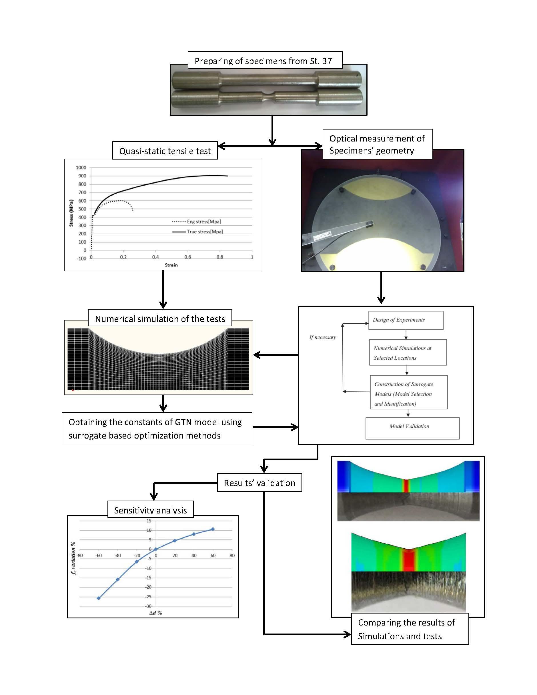
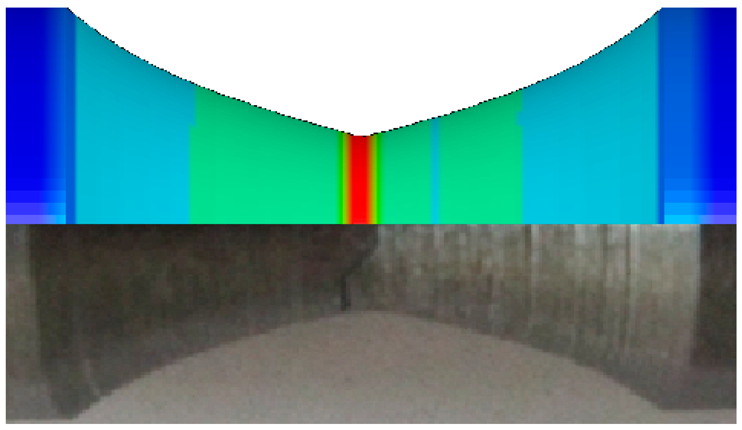
GTN damage model involves 10 constants which are normally determined by costly and time consuming experiments. It was shown in this work that the constants can be identified using a combined experimental/numerical/optimization technique which requires only two quasi-static and dynamic tensile tests to be carried out. The profiles of the specimen after fracture are obtained using a projector. The quasi-static and dynamic tests are simulated using a finite element code and the profiles of the specimen are predicted for some sets of the constants of the damage model. The difference between the numerical and the experimental specimen profiles is defined as the objective function and is optimized using the polynomial regression and Kriging methods. The constants corresponding to the optimized objective function are the answer.

2

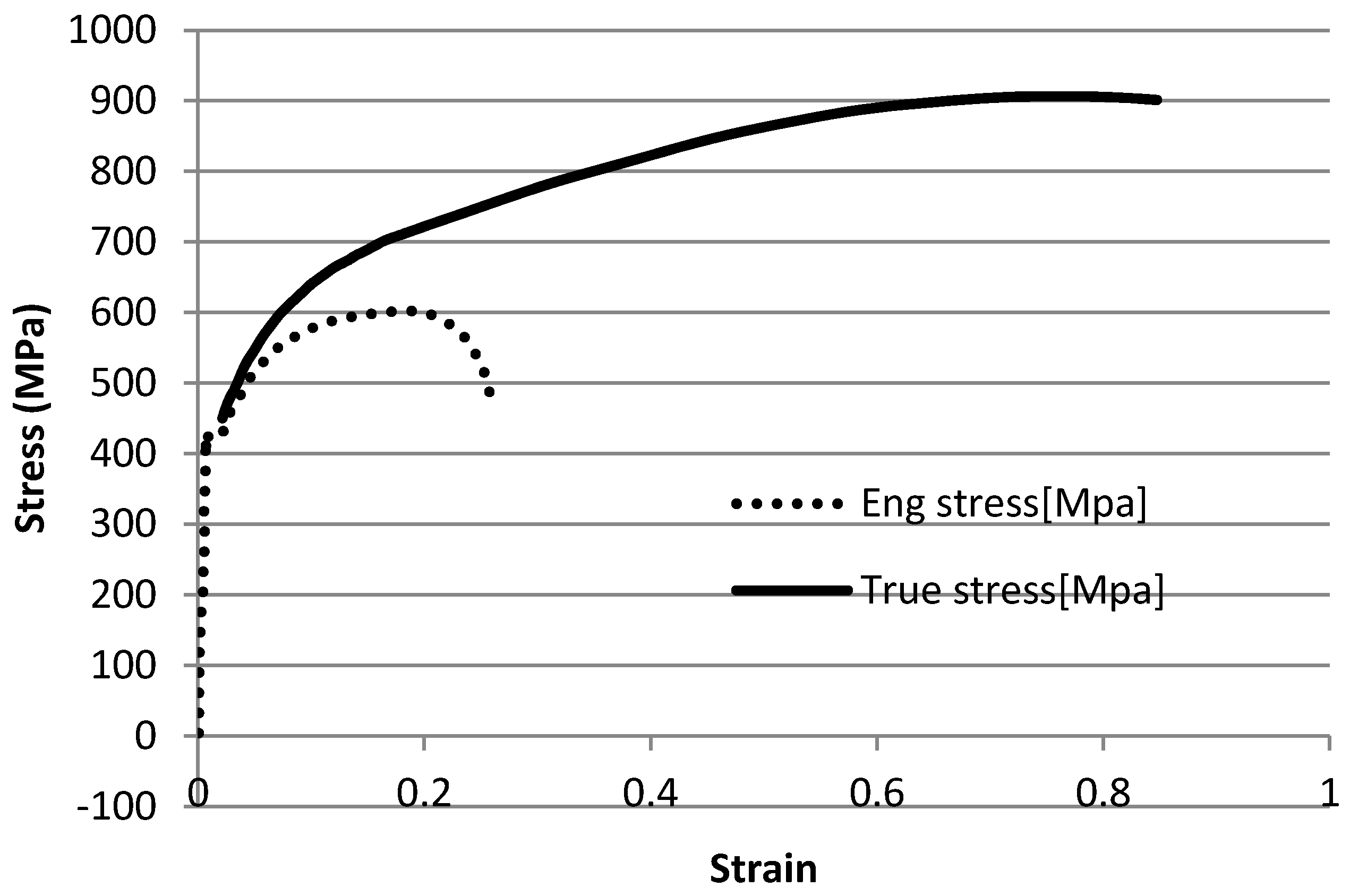
The constants σ_y, ε_y and n of GTN model can be easily computed from the stress-strain curve obtained simply from a quasi-static tensile test.

3

Kriging surrogate method is more efficient than the polynomial regression surrogate method in the sense that it provides more precise results with a smaller number of initial samples.

4

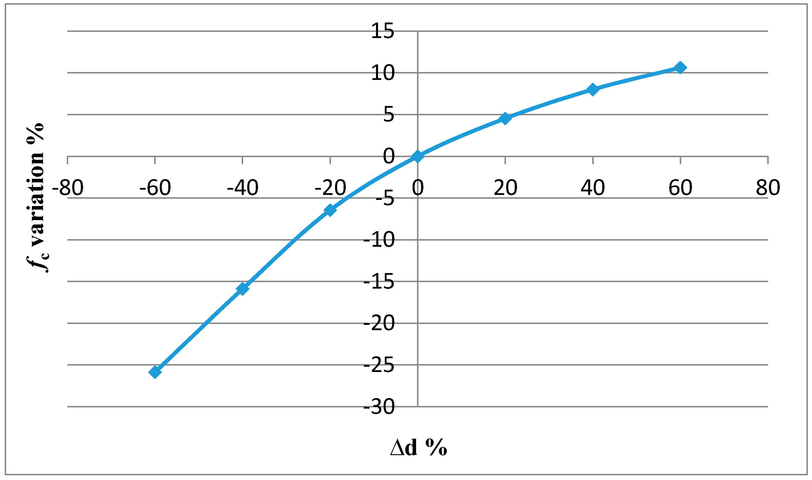
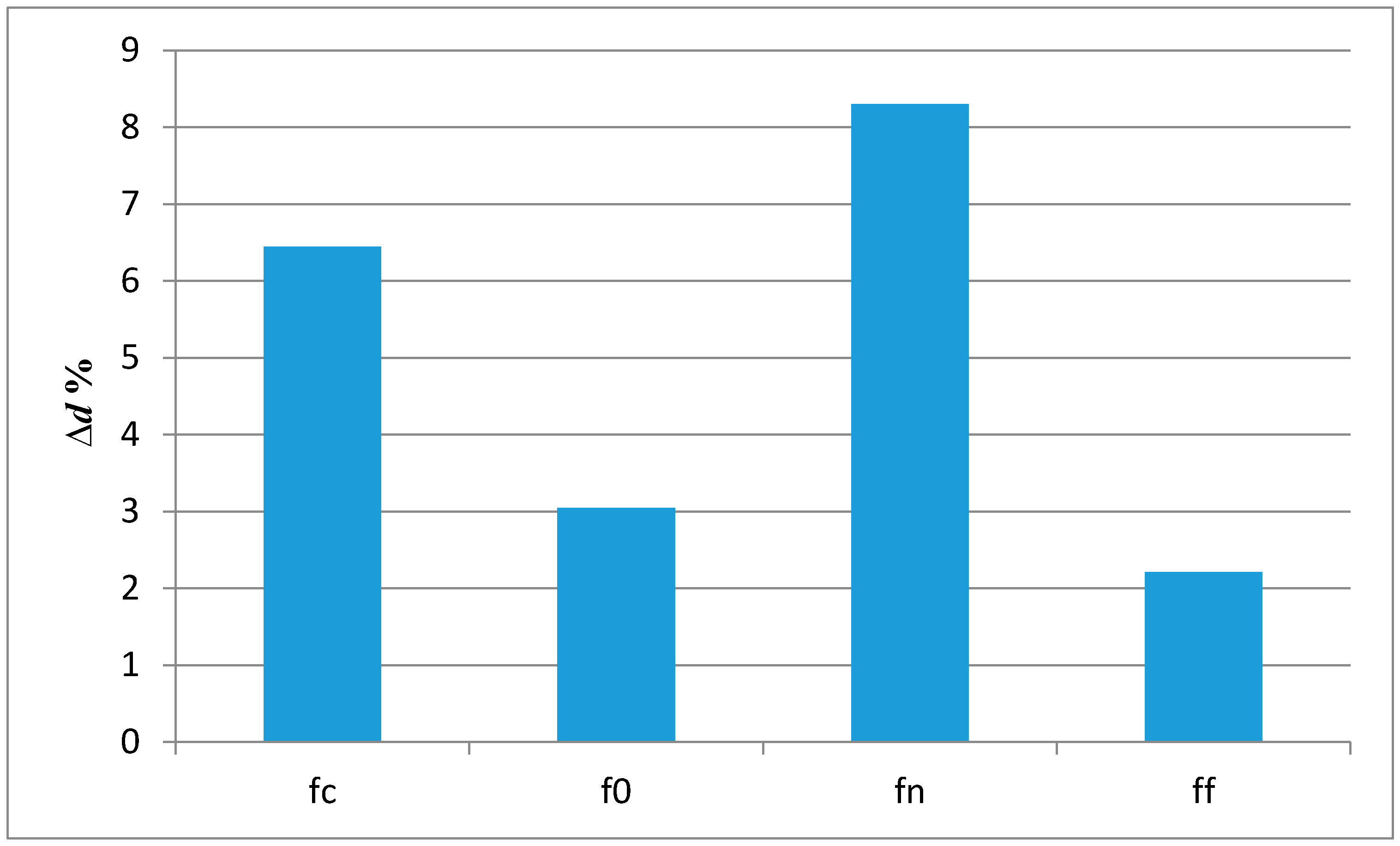
It was shown that except for the constant f_n the reduction in diameter of the specimen predicted by numerical simulation was significantly sensitive to the constants f₀, f_c and f_f.

5

Despite the fact that GTN model is an analytical method and Johnson–Cook model is an empirical method, they both provided the same accuracy in this work.

References

1. Gurson, A.L. Plastic Flow and Fracture Behavior of Ductile Materials Incorporating Void Nucleation, Growth and Interaction. Ph.D. Thesis, Brown University, Providence, RI, USA, 1975. [Google Scholar]
2. Nahshon, K.; Hutchinson, J.W. Modification of the Gurson Model for shear failure. Eur. J. Mech. A/Solids 2008, 27, 1–17. [Google Scholar] [CrossRef]
3. Vaz, M., Jr.; Muñoz-Rojas, P.A.; Cardoso, E.L.; Tomiyama, M. Considerations on parameter identification and material response for Gurson-type and Lemaitre-type constitutive models. Int. J. Mech. Sci. 2016, 106, 254–265. [Google Scholar] [CrossRef]
4. Oh, C.K.; Kim, Y.J.; Baek, J.H.; Kim, Y.P.; Kim, W. A phenomenological model of ductile fracture for API X65 steel. Int. J. Mech. Sci. 2007, 49, 1399–1412. [Google Scholar] [CrossRef]
5. Malcher, L.; Reis, F.J.P.; Andrade Pires, F.M.; César de Sá, J.M.A. Evaluation of shear mechanisms and influence of the calibration point on the numerical results of the GTN model. Int. J. Mech. Sci. 2013, 75, 407–422. [Google Scholar] [CrossRef]
6. Johnson, G.R.; Cook, W.H. Fracture characteristics of three metals subjected to various strains, strain rates, temperatures and pressures. Eng. Fract. Mech. 1985, 21, 31–48. [Google Scholar] [CrossRef]
7. Boyer, J.C.; Vidal-Salle, E.; Staub, C. A shear stress dependent ductile damage models. Int. J. Mater. Process. Technol. 2003, 121, 87–93. [Google Scholar] [CrossRef]
8. Weck, A.; Seguarado, J.; Lorca, J.L.; Wilkinson, D. Numerical simulations of void linkage in model materials using a nonlocal ductile damage approximation. Int. J. Fract. 2007, 148, 205–219. [Google Scholar] [CrossRef] [Green Version]
9. Majzoobi, G.H.; Hosseini, A.; Shahvarpour, A. An investigation into ductile fracture of ST37 Steel and pure copper at high strain rates: Part I: Experiments. Steel Res. Int. 2008, 79, 685–692. [Google Scholar]
10. Majzoobi, G.H.; Hosseini, A.; Shahvarpour, A. An investigation into ductile fracture of ST37 Steel and pure copper at high strain rates: Part II: Simulation. Steel Res. Int. 2008, 79, 712–718. [Google Scholar]
11. Ockewitz, A.; Sun, D.-Z. Damage modeling of automobile components of aluminum materials under crash loading. In Proceedings of the LS-DYNA Anwenderforum, Ulm, Germany, 12–13 October 2006. [Google Scholar]
12. Feucht, M.; Sun, D.-Z.; Erhart, T.; Frank, T. Recent development and applications of the Gurson model. In Proceedings of the LS-DYNA Anwenderforum, Ulm, Germany, 12–13 October 2006. [Google Scholar]
13. Springmann, M.; Kuna, M. Identification of material parameters of the Gurson-Tevergaard-Needleman model by combined experimental and numerical techniques. Comput. Mater. Sci. 2005, 33, 501–509. [Google Scholar] [CrossRef]
14. Broggiato, G.B.; Campana, F.; Cortes, L. Parameter identification of a material damage model: Inverse approach by the use of digital image processing. In Proceedings of the 22nd DANUBIA-ADRIA Symposium of Experimental Methods in Solid Mechanics, Parma, Italy, 28 September–1 October 2005. [Google Scholar]
15. Kuna, M.; Springmann, M. Determination of ductile damage parameters by local deformation fields. Damage Mech. Fract. Nano Eng. Mater. Struct. 2006, 535–536. [Google Scholar] [CrossRef]
16. Majzoobi, G.H. The Experimental and Numerical Study of Mechanical Behavior of Materials. Ph.D. Thesis, University of Leeds, Leeds, UK, 1990. [Google Scholar]
17. Majzoobi, G.H.; Barton, D.C.; Ramezani, M. Stress wave effects in the Flying Wedge high strain rate tensile testing device. J. Strain Anal. Eng. Des. 2007, 42, 507–516. [Google Scholar] [CrossRef]
18. Majzoobi, G.H.; Saniee, F.F.; Khosroshahi, S.; Beikmohammadloo, H. Determination of materials parameters under dynamic loading. Part I: Experiments and simulations. Comput. Mater. Sci. 2010, 49, 192–200. [Google Scholar] [CrossRef]
19. Majzoobi, G.H.; Saniee, F.F.; Khosroshahi, S.; Beikmohammadloo, H. Determination of materials parameters under dynamic loading. Part II, Optimization. Comput. Mater. Sci. 2010, 49, 201–208. [Google Scholar] [CrossRef]
20. Jones, D.R.; Schonlau, M.; William, J. Efficient global optimization of expensive black-box functions. J. Glob. Optim. 1998, 13, 455–492. [Google Scholar] [CrossRef]
21. Regis, R.G. Particle swarm with radial basis function surrogates for expensive black-box optimization. J. Comput. Sci. 2014, 5, 12–23. [Google Scholar] [CrossRef]
22. Mack, Y.; Goel, T.; Shyy, W.; Haftka, R. Surrogate model-based optimization framework: A case study in aerospace design. In Evolutionary Computation in Dynamic and Uncertain Environments; Yang, S., Ong, Y.-S., Jin, Y., Eds.; Springer: Berlin, Germany, 2007; pp. 323–342. [Google Scholar]
23. Holmstr, K.; Quttineh, N.; Edvall, M.M. An adaptive radial basis algorithm (ARBF) for expensive black-box mixed-integer constrained global optimization. Optim. Eng. 2008, 9, 311–339. [Google Scholar] [CrossRef]
24. Han, Z.H.; Zhang, K.S. Surrogate-based optimization. In Real-World Applications of Genetic Algorithms; Roeva, O., Ed.; InTech: New York, NY, USA, 2008; pp. 343–362. [Google Scholar]
25. Wang, C.; Duan, Q.; Gong, W.; Ye, A.; Di, Z.; Miao, C. An evaluation of adaptive surrogate modeling based optimization with two benchmark problems. Environ. Model. Softw. 2014, 60, 167–179. [Google Scholar] [CrossRef]
26. Queipo, N.V.; Haftka, R.T.; Shyy, W.; Goel, T.; Vaidyanathan, R.; Tucker, P.K. Surrogate-based analysis and optimization. Prog. Aerosp. Sci. 2005, 41, 1–28. [Google Scholar] [CrossRef]
27. Persson, J. Design and Optimization under Uncertainties a Simulation and Surrogate Model Based Approach. Ph.D. Thesis, Linkoping University, Linkoping, Sweden, 2012. [Google Scholar]
28. Draper, N.R.; Smith, H. Applied Regression Analysis, 3rd ed.; Wiley: New York, NY, USA, 1998. [Google Scholar]
29. Wilkins, M.L.; Streit, R.D.; Reaugh, J.E. Cumulative-Strain-Damage Model of Ductile Fracture: Simulation and Prediction of Engineering Fracture Test; UCRL-53058 Distribution Category UC-25; Lawrence Livermore Laboratory: Livermore, CA, USA; University of California: Oakland, CA, USA, 1980.
30. Needleman, A.; Tvergaard, V. An analysis of ductile rupture in notched bars. J. Mech. Phys. Solids 1984, 32, 461–490. [Google Scholar] [CrossRef]
31. Sun, D.Z.; Honi, A.; Bohem, W.; Shmitt, W. Application of micromechanical models to the analysis of ductile fracture under dynamic loading. Fruct. Mech. 1995, 25, 343–357. [Google Scholar]
32. Abbassi, F.; Belhadj, T.; Mistou, S.; Zghal, A. Parameter identification of a mechanical ductile damage using Artificial Neural Networks in sheet metal forming. Mater. Des. 2012, 45, 605–615. [Google Scholar] [CrossRef] [Green Version]
33. Bridgman, P.W. Studies in Large Plastic Flow and Fracture; Harvard University Press: Cambridge, MA, USA, 1964. [Google Scholar]
34. Majzoobi, G.H.; Dehgolan, F.R. Determination of the constants of damage models. Procedia Eng. 2011, 10, 764–773. [Google Scholar] [CrossRef]
35. Johnson, G.R.; Cook, W.H. A constitutive model and data for metals subjected to large strain, high strain rate and high temperature. In Proceedings of the 7th International Symposium on Ballistics, The Hague, The Netherlands, 19–21 April 1983; pp. 541–547. [Google Scholar]
Figure 1. The schematic pictures of plain and notched specimens.
Applsci 07 01179 g001
Figure 2. The true and engineering stress-strain curves.
Applsci 07 01179 g002
Figure 3. Flying Wage testing apparatus
Applsci 07 01179 g003
Figure 4. Dynamic test specimens.
Applsci 07 01179 g004
Figure 5. Projected picture of the specimen on the projector screen.
Applsci 07 01179 g005
Figure 6. Finite element model of the specimen in notch area.
Applsci 07 01179 g006
Figure 7. A view of 3-D model of the Flying Wedge
Applsci 07 01179 g007
Figure 8. A view of finite element model of the Flying Wedge.
Applsci 07 01179 g008
Figure 9. The 3-D model of the specimen for dynamic test highlighting the notch area.
Applsci 07 01179 g009
Figure 10. The finite element model of the specimen for dynamic test highlighting the notch area.
Applsci 07 01179 g010
Figure 11. The flow chart of the surrogate-based optimization method.
Applsci 07 01179 g011
Figure 12. A schematic of six sample points selection using LHS method.
Applsci 07 01179 g012
Figure 13. A comparison between the profiles of specimen measured from numerical simulation and quasi-static test.
Applsci 07 01179 g013
Figure 14. A comparison between the profiles of specimen measured from numerical simulation and dynamic test.
Applsci 07 01179 g014
Figure 15. The location of voids’ initiation and coalescence predicted by GTN Model.
Applsci 07 01179 g015
Figure 16. Sensitivity of diameter reduction vs. f0.
Applsci 07 01179 g016
Figure 17. Sensitivity of diameter reduction vs. fn.
Applsci 07 01179 g017
Figure 18. Sensitivity of diameter reduction vs. fc.
Applsci 07 01179 g018
Figure 19. Sensitivity of diameter reduction vs. ff.
Applsci 07 01179 g019
Figure 20. Variation of the ∆d for 20% change in each constants of GNT model.
Applsci 07 01179 g020