Comparison of Training Approaches for Photovoltaic Forecasts by Means of Machine Learning


Dipartimento di Energia, Politecnico di Milano, via La Masa 34, 20156 Milano, Italy
*
Author to whom correspondence should be addressed.
†
These authors contributed equally to this work.
Appl. Sci. 2018, 8(2), 228; https://0-doi-org.brum.beds.ac.uk/10.3390/app8020228
Submission received: 31 December 2017
/
Revised: 24 January 2018
/
Accepted: 28 January 2018
/
Published: 2 February 2018
(This article belongs to the Special Issue Computational Intelligence in Photovoltaic Systems)
Abstract
:The relevance of forecasting in renewable energy sources (RES) applications is increasing, due to their intrinsic variability. In recent years, several machine learning and hybrid techniques have been employed to perform day-ahead photovoltaic (PV) output power forecasts. In this paper, the authors present a comparison of the artificial neural network’s main characteristics used in a hybrid method, focusing in particular on the training approach. In particular, the influence of different data-set composition affecting the forecast outcome have been inspected by increasing the training dataset size and by varying the training and validation shares, in order to assess the most effective training method of this machine learning approach, based on commonly used and a newly-defined performance indexes for the prediction error. The results will be validated over a one-year time range of experimentally measured data. Novel error metrics are proposed and compared with traditional ones, showing the best approach for the different cases of either a newly deployed PV plant or an already-existing PV facility.
1. Introduction
In recent years, several forecasting methods have been developed for the output power of renewable energy sources (RES) [1], addressing in particular the intrinsic variability of parameters related to changing weather conditions, which directly affect the photovoltaic (PV) systems’ power output [2]. This increasing attention is mainly due to the increasing shares of RES quota in power systems, which involve novel technical challenges for the efficiency of the electrical grid [3]. In particular, predictive tools based on historical data can generally provide advantages in PV plant operation [4,5], reduce excess production, and take advantage of incentives for RES production [6].
Among the commonly-used forecasting models, most aim to predict the expected power production based on numerical weather prediction (NWP) systems forecasts [7]. This is a complex problem with high degrees of non-linearity; for this reason, it is commonly approached by means of advanced models and techniques—i.e., evolutionary computation [8], machine learning (ML) [9], and artificial neural networks (ANNs) [10]. These are pseudo-stochastic iterative approaches defined in the class of computational intelligence techniques, and are usually employed to address pattern recognition, function approximation, control, and forecasting problems [11]. Moreover, they are generally able to handle incomplete or missing data and solve problems with a high degree of complexity.
Recently, several ANN layouts have been developed to solve different tasks [12], such as: times series prediction, complex dynamical system emulation [13], speech generation, handwritten digit recognition, and image compression, due to their ability to learn from extended time series of historical measurements with acceptable error levels compared to other statistical and physical forecasting models [14]. Currently, ANN employment in forecasting is quite straightforward due to the widespread development of specific software applications [15,16,17].
In particular, the first attempts at solar power forecasting by means of ANN started more than a decade ago [18]. Generally, in the case of PV power output, common training data are the historical measurements of power production from a PV facility and meteorological parameters unique to the facility location, including temperature, global horizontal irradiance (i.e., the intensity of all the solar radiation components on a horizontal surface) [19], and cloud cover above the facility. Additional forecasted variables from the numerical weather predictions can also be considered, such as wind speed, humidity, pressure, etc. [20].
Novel forecasting models were recently implemented by adding an estimate of the clear sky radiation to the series of historical local weather data, as reported in [21].
Additionally, the effectiveness of ensemble methods was demonstrated in [22], thus giving additional advantages in terms of results reliability and the implementation of efficient parallel computing techniques.
In their previous work [23], the authors conducted a detailed analysis to find a procedure for the best ANN layout and settings in terms of the number of layers, neurons, and trials for the PV day-ahead forecast. Furthermore, evidence showed that the forecasting performance of ML techniques is affected by the composition of the training data-set, as well as by input selection [24,25].
In this paper, a specific study is conducted on training data-sets in order to provide a more detailed analysis of the effect of different approaches in the training data-set composition on the day-ahead forecast of the PV power production. In particular, the authors present some procedures to set-up the training and validation data-sets for the ANN used in physical hybrid method to perform the day-ahead PV power forecast in view of the electricity market. Moreover, a novel error metric is proposed and compared with traditional ones, in order to validate the best training approach in different cases: indeed, the procedures outlined herein can be adopted to set-up data-sets based on either historical data retrieved from an existing PV plant or on incremental data measurements in a newly deployed PV plant. The test data set will be made up of the 24-hourly PV power values forecasted one day-ahead.
The paper is structured as follows: Section 2 provides an overview of the considered approaches for the composition of the training database, considering both cases of historical data retrieved from an existing PV plant and incremental data measurements in a newly deployed PV plant; Section 3 presents the methodology implemented to compare the different training approaches presented here, proposing some new metrics aimed at evaluating the suitability of the proposed configurations in terms of error performance and statistical behavior; Section 4 presents the considered case study, which is used to test the proposed training approaches: specific simulations and numerical results are provided in Section 5, and final remarks are reported in Section 6.
2. Training Database Composition Approaches
In order to perform the day-ahead forecast, the ANN needs to be trained. Hence, the amount of historical data employed in the supervised learning determines the ANN forecast capability. This amount of data is formed of samples exploited in the process of identifying the links among neurons in the network which minimize the error in the forecast. In order to do this task, the whole amount of available samples is divided in two groups:
- the “training set” (or equally “training database”), which is used to adjust the weights among neurons by performing the forecast on the same samples,
- the “validation set”, which is used as a stopping criteria to avoid over-fitting and under-fitting. It proves the goodness of the trained network on additional samples which have not been previously included in the training set. The purpose of this step is to test the generalization capability of the neural network on a new data-set.
Learning occurs by updating elements within the network; thus, its response iteratively improves to match the desired output. An ANN is trained when it has learned its task and converges to a solution. To achieve this, some learning algorithms are commonly used:
- error back-propagation (EBP)
- gradient descent
- conjugate gradient
- evolutionary algorithms (genetic algorithms, particle swarm optimization, etc.)
Sometimes, according to the problem, the fastest algorithm gives solutions rapidly converging on local minima; however, this does not guarantee the maximum accuracy. In addition, it should be considered that a large training set size provides a better sample of the trends improving generalization, but it generally slows down the learning process. If an ANN is not properly trained or sized, there are usually undesired results, such as “overfitting” and “underfitting” [26]. Using ANN ensembles by averaging their outputs has been demonstrated to be beneficial, as it helps to avoid chance correlations and the overtraining problem [27,28].
However, to choose both the most suitable learning algorithm and the proper size of the training set which minimizes the error is a challenge which should be faced in each case study [29,30,31].
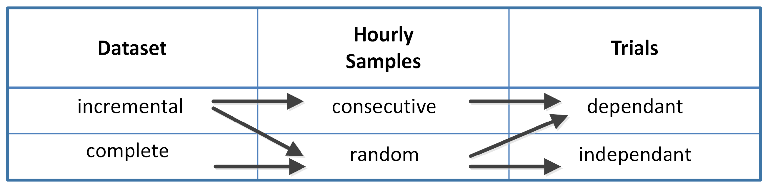
In this paper, we inspect how the behavior on the day-ahead forecast is influenced by the possible characteristics summarized in Figure 1. The first characteristic of the data-set is either “incremental” when the elements belonging to the training data-set are progressively available over time and the training set size gradually increases or “complete” if an already existing database of samples is available. The second characteristic refers to the way the data-set is used for training the ANN. As the forecast-making is mainly a stochastic process, the choice could be to use entirely the same training data set for each forecast of the ensemble (we refer to the single forecast with the term “trial”, and in this case, all the trials will be the same in the ensemble) or to shuffle its elements, grouping them in smaller subsets adopted each time to separately train a different ANN (in this other case, each trial is independent, as all the training data-sets are different). Finally, the mean of the resulting output is usually calculated in the so-called “ensemble” forecast. The third characteristic is related to the order of the hourly samples that constitute the training data-set. They can appear either consecutively displaced as the chronological time series they belong to or they can be randomly grouped and mixed up.
The combination of these characteristics results in different ANN training methods, which could affect the forecast.
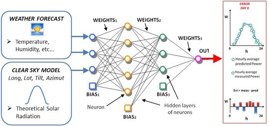
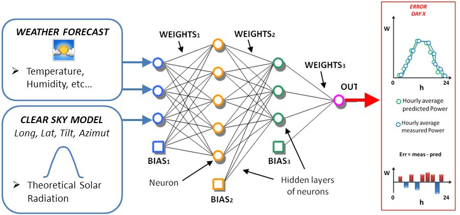
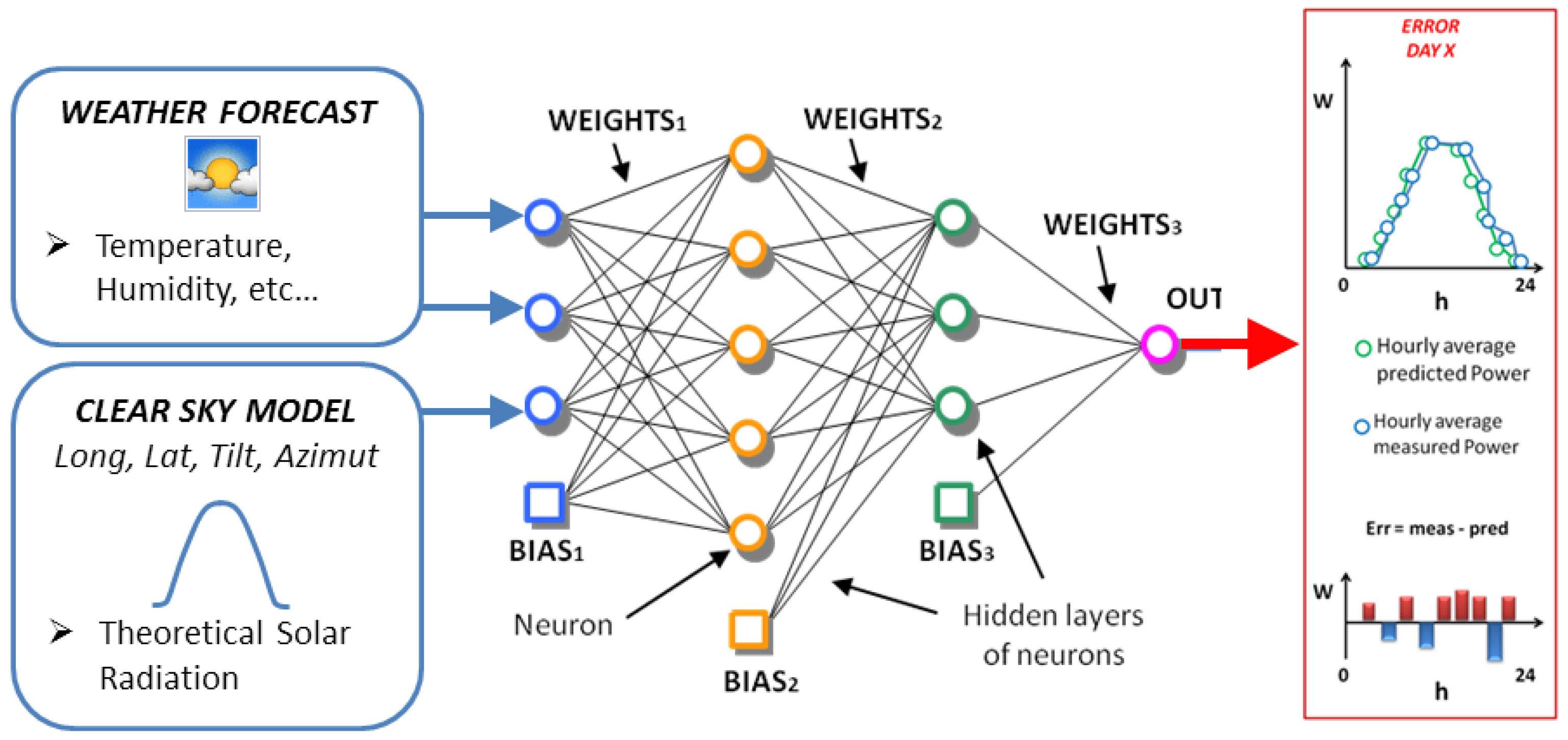
All of the assumptions exposed here are valid, in general terms, for all ANN-based methods. In this specific paper, authors employ the Physical Hybrid Artificial Neural Network (PHANN) method for the day-ahead forecast, as described in detail in [14,21]. This procedure mixes the physical Clear Sky Radiation Model (CSRM) and the stochastic ANN method as reported in Figure 2.
2.1. Incremental Training Data-Set
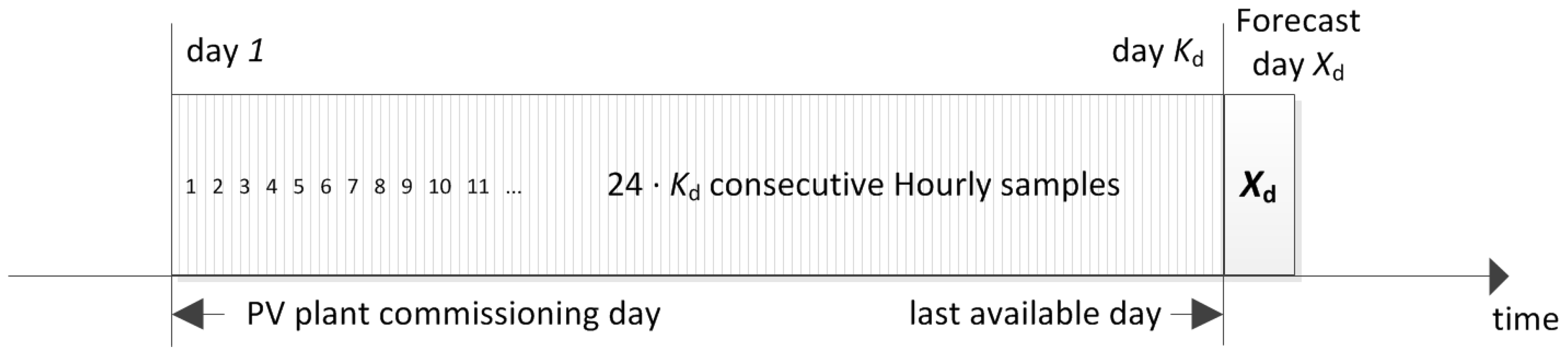
An incremental data-set occurs when the available samples are limited. Usually this is the case of real-time or time-dependant processes, and data can be acquired only progressively. Consider for example our case study when the monitoring system starts recording data from the first day of operation of the PV plant: initially a small amount of data is recorded, and if we acquire hourly samples, 24 samples are added to the historical data-set every day.
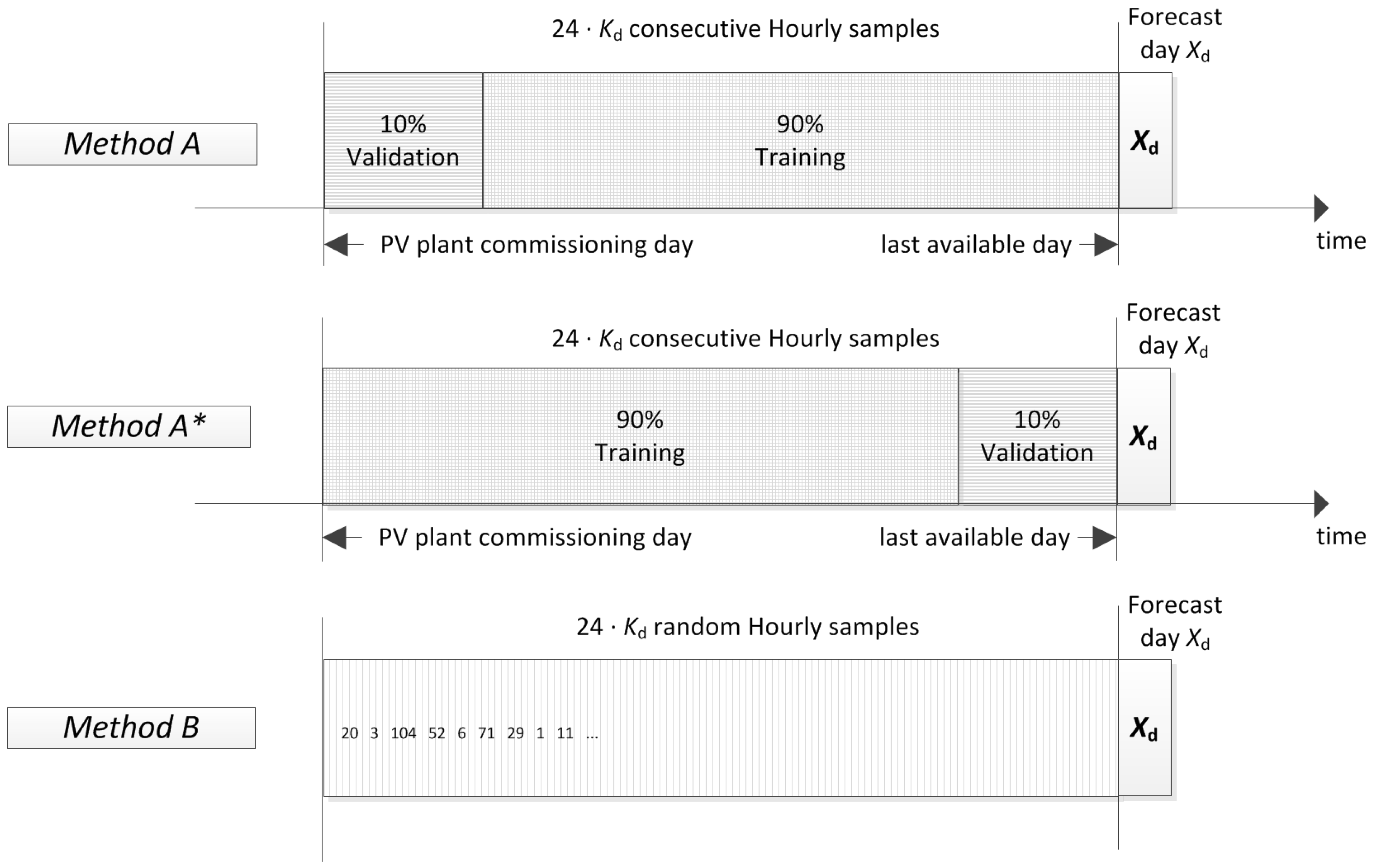
In this database composition (e.g., see Figure 3), the days which can be employed for ANN training are those available starting from the PV plant commissioning (day 1) until the day before the forecast (day ). As a consequence, the size of the training database will increase over time. In order to supply the data-set to the network for the training step, samples can be arranged in different methods. Those adopted in this paper are listed in Figure 4, and determine different results in the forecast. A short description is given in the following:
- Method A employs the same chronologically consecutive samples by grouping the 90% of the samples which are closest to the forecast day for the training set and the remaining 10% of the samples for the validation set.
- Method A* employs the same chronologically consecutive samples by grouping the 90% of the samples for the training set and the 10% of the samples which are closest to the forecast day for the validation set.
- Method B employs the samples by randomly grouping them separately, 90% for the training set and 10% for the validation set.
In the first two methods (A and A*), the effect of the proximity of the training set to the forecast day is examined (implying seasonal variations on the parameter), inspecting how the forecast is affected by the proximity of the samples employed in the training rather than in the validation step. For example, it is clear that forecasting spring days cannot be accurate if the training samples belong to the past autumn or winter, and the same consideration applies for the validation. Reasonably, we are expecting that the further the samples of the validation are, the less accurate the forecast. Obviously, this problem is not addressed in Method B, as samples are randomly chosen.
2.2. Complete Training Data-Set
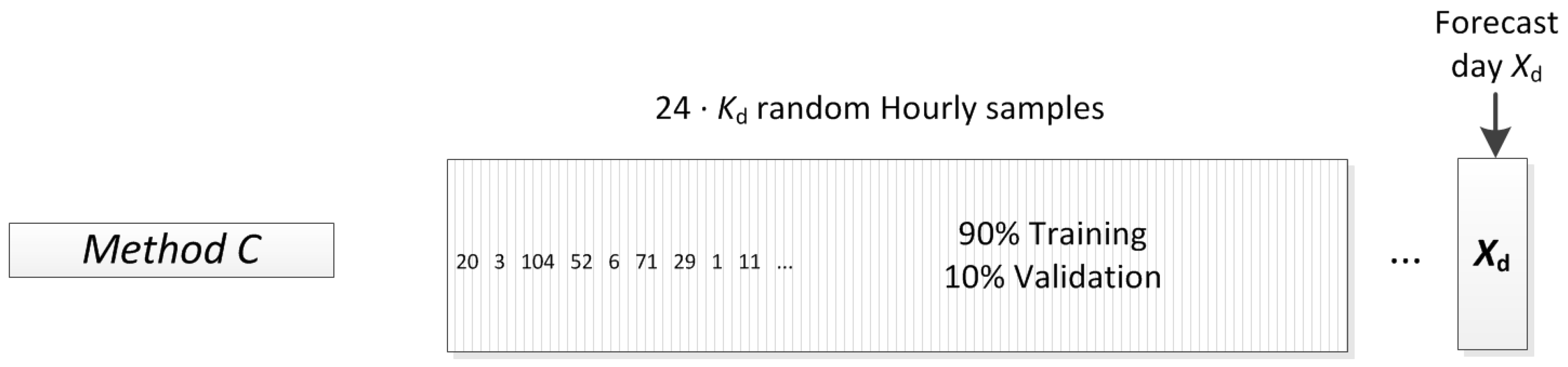
In the complete data-set, an extended amount of samples is available, but it might belong to a period of time which is time-wise distant from the days of the forecast, as it is shown in Figure 5. In this case, samples which have to be employed for the ANN training can either be mixed (as shown in Figure 6) each time that a trial is performed (this happens when trials are independent with Method C1), or each trial depends on the same training data-set with Method C2.
The complete list of the training methods which have been adopted in this paper is in Table 1. The different shares of the training and the validation set, 90% and 10%, respectively, have been set up in previous works.
3. Evaluation Indexes
The effect of the different methods of training is investigated by means of some evaluation indexes. These indexes aim at assessing the accuracy of the forecasts and the related error, and it is therefore necessary to define the indexes. There is a wide variety of existing definitions of the forecasting performance, and technical papers present many of these indexes; hence, we will report some of the most commonly used definitions in the literature ([32,33,34]).
The hourly error is the starting definition given as the difference between the hourly mean values of the power measured in the h-th hour and the forecast provided by the adopted model [32,35]:
From the hourly error expression and its absolute value , other definitions can be inferred; i.e., the well-known mean absolute percentage error ():
where N represents the number of samples (hours) considered: usually it is calculated for a single day, month, or year.
Since the hourly measured power significantly changes during the same day (i.e., sunrise, noon, and sunset), for the sake of a fair comparison, in this paper the authors preferred to consider the normalized mean absolute error :
where the percentage of the absolute error is referred to the rated power C of the plant, in place of the hourly measured power .
In this paper we also adopted the mean value of all the , which refers to the d-th day, calculated over the whole period. Therefore, we introduce , which is the mean of all the daily obtained with a given data-set:
The weighted mean absolute error is based on total energy production:
The normalized root mean square error is based on the maximum hourly power output :
This error definition is the well-known root mean square error () which has been normalized over the maximum hourly power output measured in the considered time range, for the sake of a fair comparison.
is largely used to evaluate the accuracy of predictions and trend estimations. In fact, often relative errors are large because they are divided by small power values (for instance the low values associated to sunset and sunrise): in such cases, could result very large and biased, while , by weighting these values with the capacity of the plant C, is more useful.
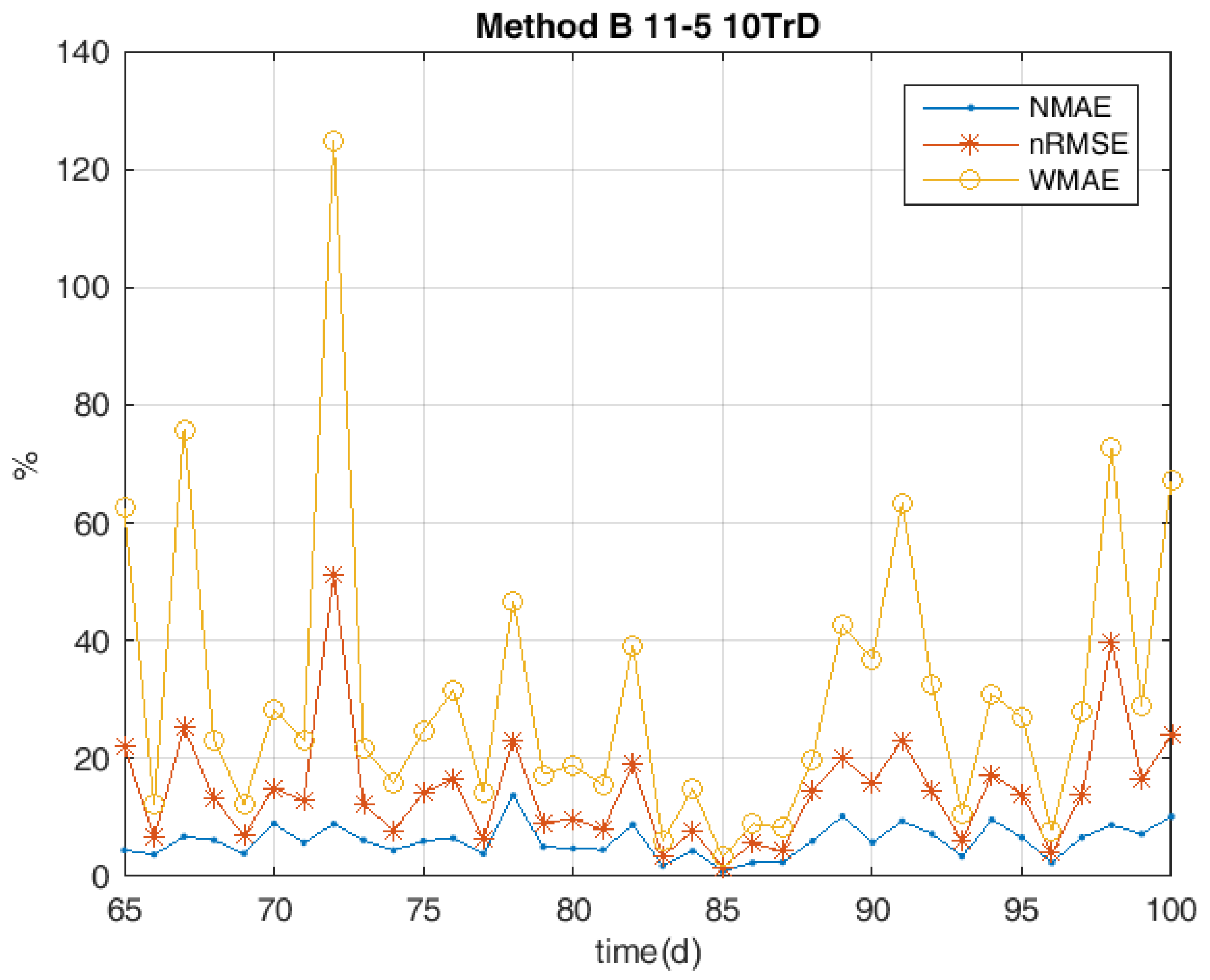
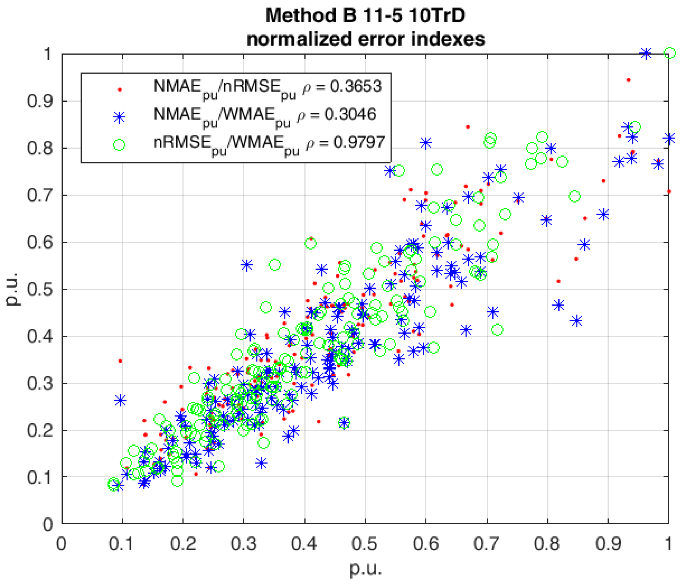
The measures the mean magnitude of the absolute hourly errors . In fact, it gives a relatively higher weight to larger errors, thus allowing particularly undesirable results to be emphasized. In fact, if we consider the daily trends of the aforementioned indexes (which are shown in Figure 7), it can be seen how they are correlated, while in the same Figure 8, the scatterplot of their normalized values with the relative maxima clearly shows these correlations between the three error indexes. Furthermore, the Pearson–Bravais correlation index [36] has been calculated to underline the direct relationship among the error indexes:
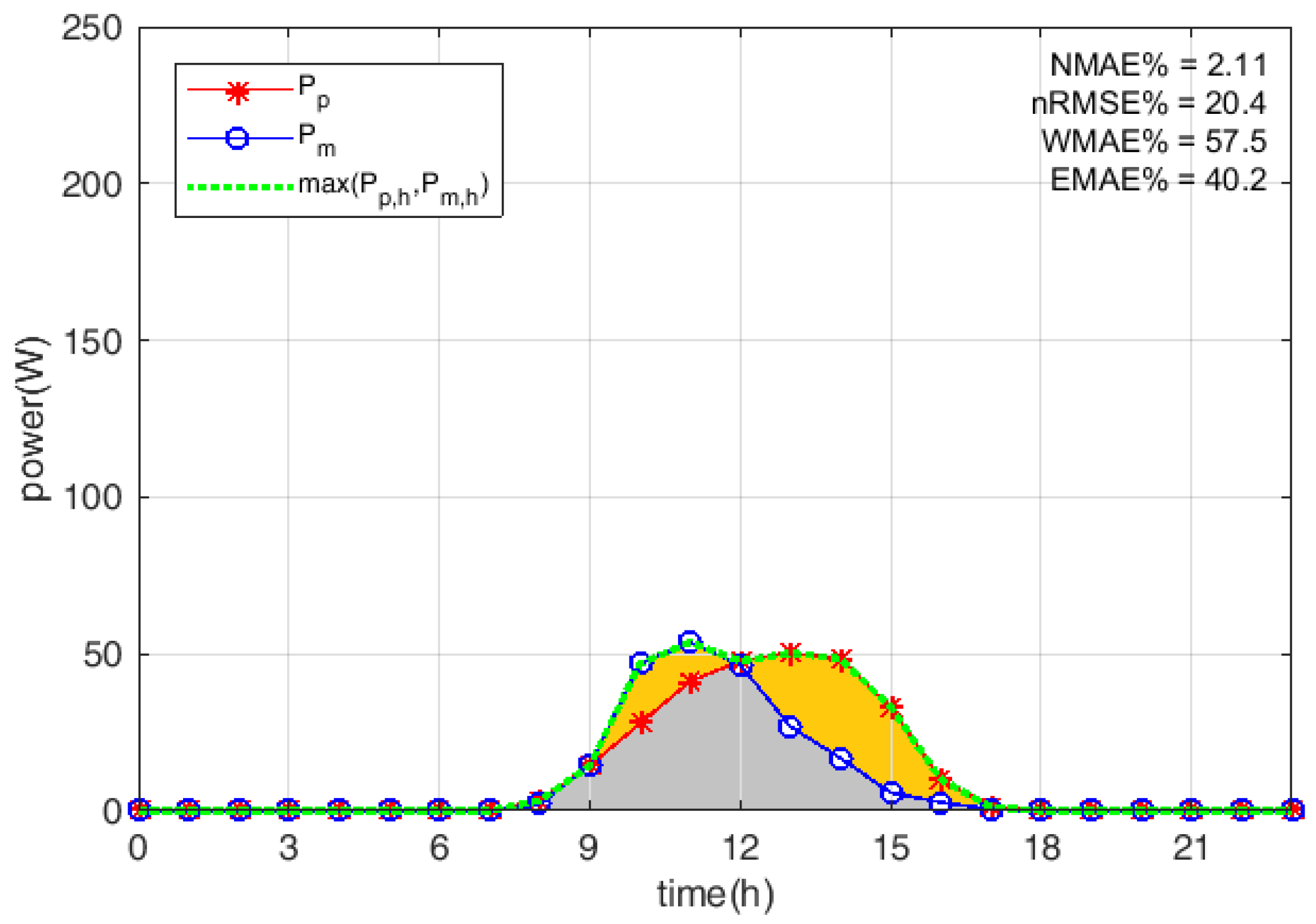
However, as it is shown in Figure 7, the daily evaluation indexes expressed in Equations (3), (5), and (6) could vary a great deal, being unable to give complete information “at a glimpse” of the accuracy of the prediction. For example, consider Figure 9 and Figure 10, where the forecasts and the relevant evaluation indexes for 1 April and 4 November 2014, respectively, are depicted. In both cases, daily values are quite low (around 2–3%) and a forecast assessment solely based on this basis could be misleading.
Actually, the 1 April was quite a sunny day and the bell-shaped hourly power curve which has been forecast—the red starred line—was accurately following the measured one—the blue circled line. The cloudy winter day 4 November 2014 was a different story; in fact, the forecast red curve is biased on the noon hours, while the actual blue curve in the morning. However, in the second day, the daily value is lower. This is owing to the normalisation of the mean absolute error with the net capacity of the plant. Regarding the other evaluation indexes, even if they are correlated, they can exceed the cap, as happens for example to in Figure 7 on day 72.
Starting from these assumptions, and in view of a more useful summary evaluation, an additional performance index is proposed, aiming to provide a value between 0% and of the forecast accuracy. Therefore the envelope-weighted mean absolute error, is defined as:
where the numerator is the sum of the absolute hourly errors, as in , while the denominator is the sum of the maximum between the forecast and the measured hourly power. In particular, this definition is consistent with a graphical representation of the error, where the numerator corresponds to the yellow area shown in Figure 9 and Figure 10 and the denominator is the sum of the gray and yellow areas highlighted in the same figures. With reference to the above-mentioned days, while the two values are nearly the same, the is in the first case and in the second case, and it never exceeds .
As with the daily , in this study we also introduced the mean value of all the , which are referred to the d-th day, calculated over the whole period. Therefore, is the mean of all the daily for a given data-set:
4. Case Study
Experimental data for this study were taken from the laboratory SolarTechLab [37] located in Milano, Italy (coordinates: N; E). In 2014, the DC output power of a single PV module with the following characteristics was recorded:
- PV technology: Silicon mono crystalline,
- Rated power (Net capacity of the PV module): 245 Wp,
- Azimuth: (assuming as south direction and counting clockwise),
- Solar panel tilt angle (): ,
The monitoring activity of the PV system parameters lasted from 8 February to 14 December 2014, but the employable data, without interruptions and discontinuities, amount to 216 days. These 24-hourly samples were used as the database for the forecasting methods comparison.
The PV module was linked to the electric grid by a micro-inverter ABB MICRO-0.25-I- OUTD [38], guaranteeing the optimization of the production. Its operating parameters—DC power included—were transmitted to a workstation for storage using a ZigBee protocol wireless connection, in real-time. An important issue that arises is how to avoid missing values and outliers. A suitable pre-processing procedure, which has already been developed and described in detail in [39], is applied here.
The weather forecasts employed were delivered by a weather service each day at 11 a.m. of the day before the forecasted one, for the exact location of the PV plant. The historical hourly database of these parameters was used to train the network and includes the following parameters:
- ambient temperature (C),
- global horizontal irradiance (W/m),
- global irradiance on the plane of the array (W/m),
- wind speed (m/s),
- wind direction (),
- P pressure (hPa),
- R precipitation (mm),
- cloud cover (%),
- cloud type (Low/Medium/High).
In addition to these parameters, in order to train the PHANN method, the local time (hh:mm) of the day and the Clear Sky Radiation model (W/m) were also provided. These are the eleven inputs of the ANN. Regarding the specific settings of the ANN, exception made for the training database composition (as presented in Section 2), they were selected on the basis of a sensitivity analysis, as outlined in a previous study [23]. The ANN settings adopted in this study were:
- neurons in the input layer: 11,
- neurons in the first hidden layer: 11,
- neurons in the second hidden layer: 5,
- neurons in the output layer: 1,
- training algorithm: Levenberg–Marquardt,
- activation function: sigmoid,
- number of trials in the ensemble forecast: 40.
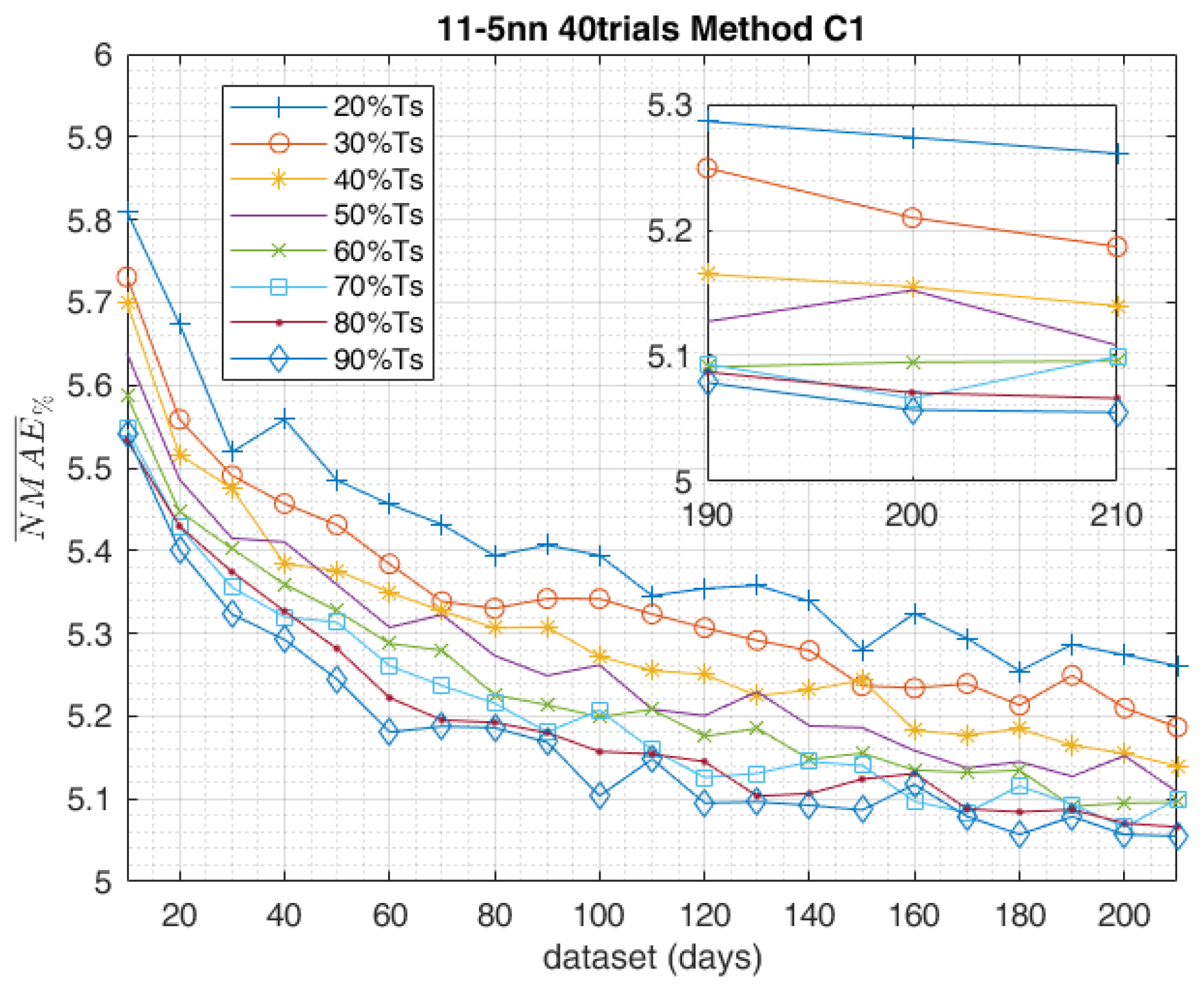
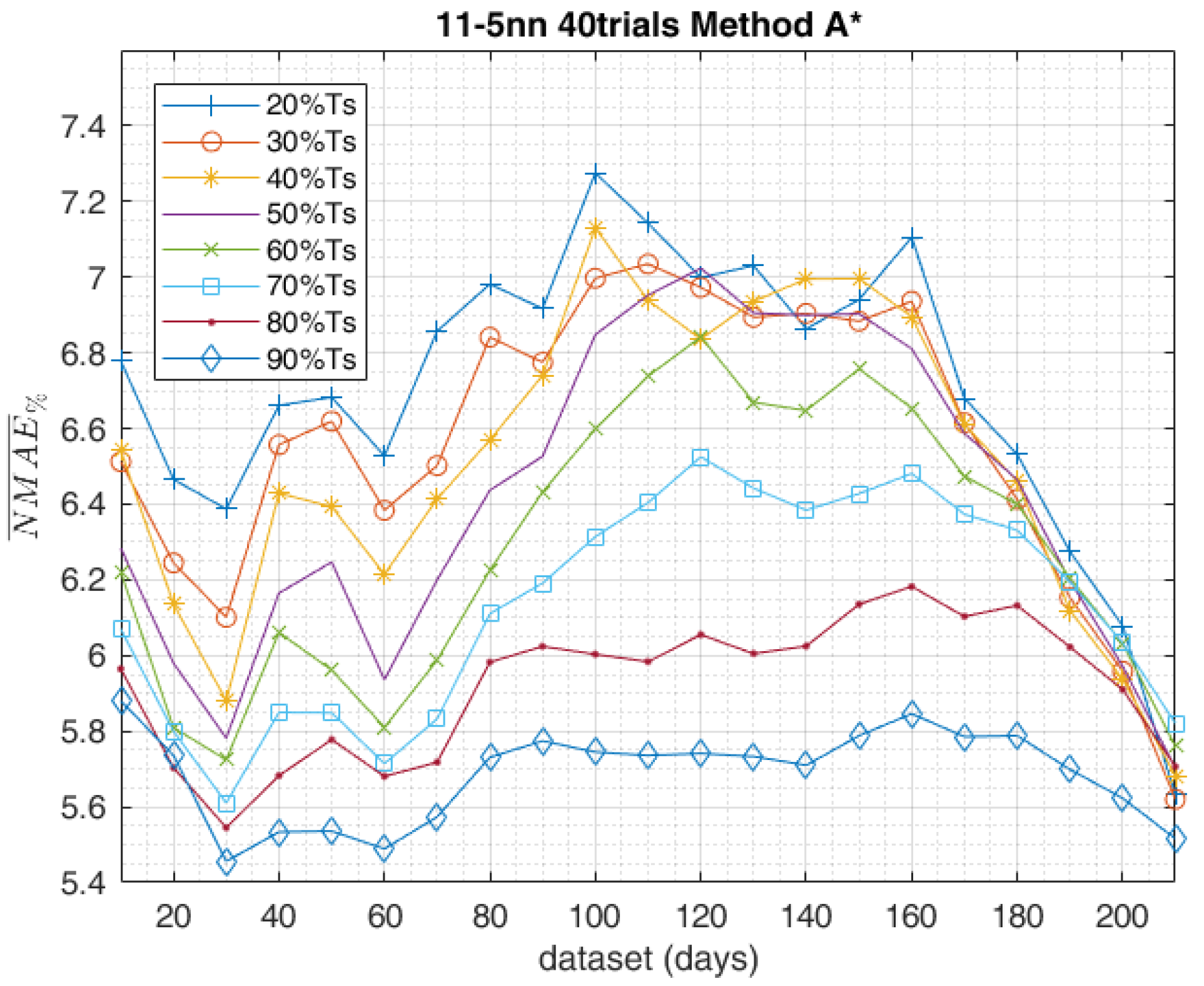
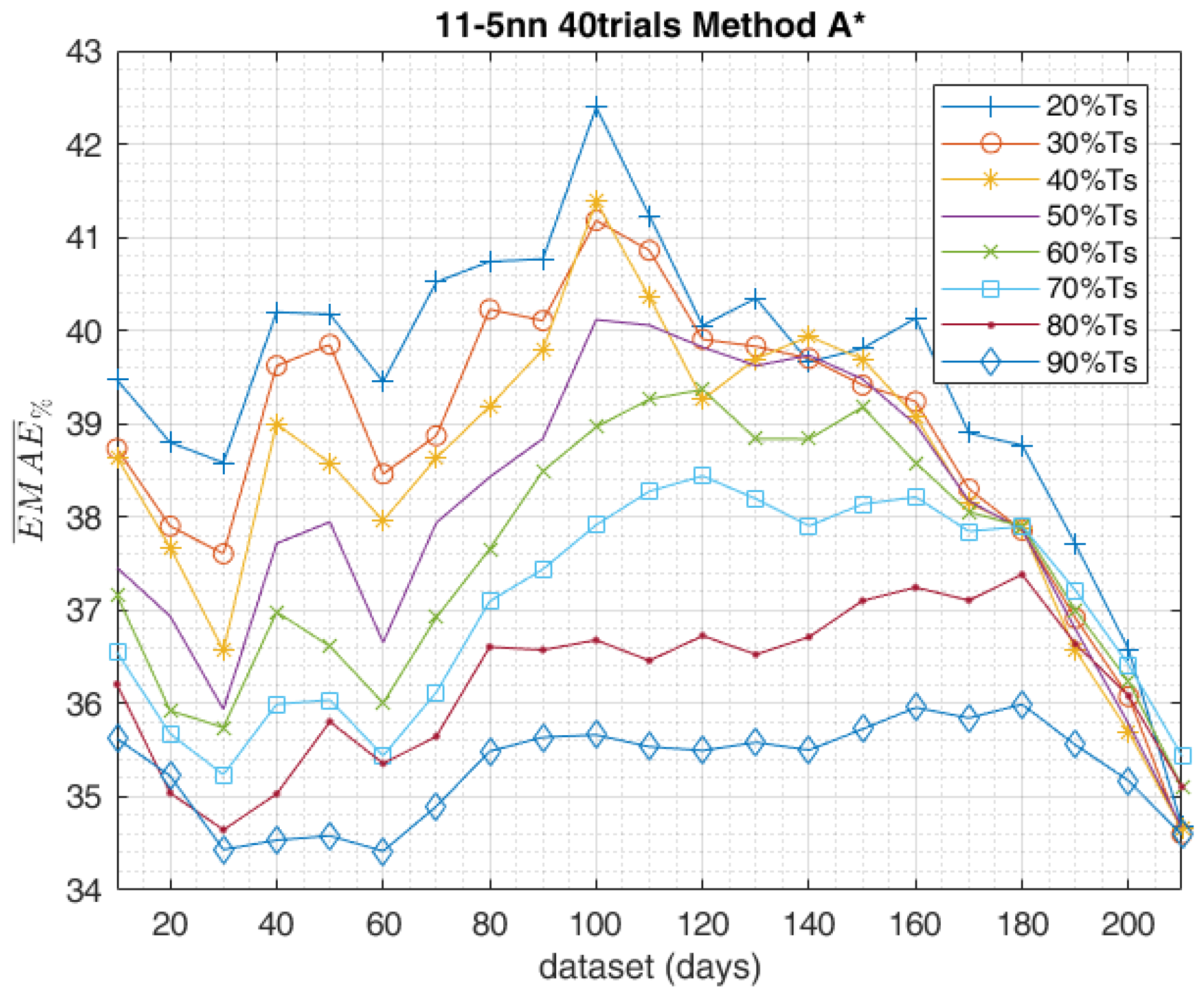
The share of the data included in the training and in the validation steps have been adjusted by means of another sensitivity analysis. Independently of how many days were employed in the training, the database was divided into two groups containing different amounts of data. Thereafter, they were provided first to train the network and the remaining data for the validation. Finally, the ensemble forecast was performed. This procedure was followed several times, progressively increasing the number of days employed in the training-process. The above-mentioned performance indexes over the whole year were calculated, and according to the different shares adopted between training and validation, the results are plotted in Figure 11 and Figure 12. The results depicted here refer to the training method C1, and the reason for this choice will be explained later in Section 5. As can be seen, the best results are always guaranteed by adopting of data for the training and the remaining for the validation (the blue rhomboidal curve). However, the zoom in the top-right corner of Figure 11 shows that, for the largest amount of data (210 days), also of data for the training and for the validation (the purple dotted curve) provided similar results to the previously described curve. The same trends were obtained in Figure 12, where the trend of is shown as a function of the data-set size and the shares of training and validation set.
5. Results
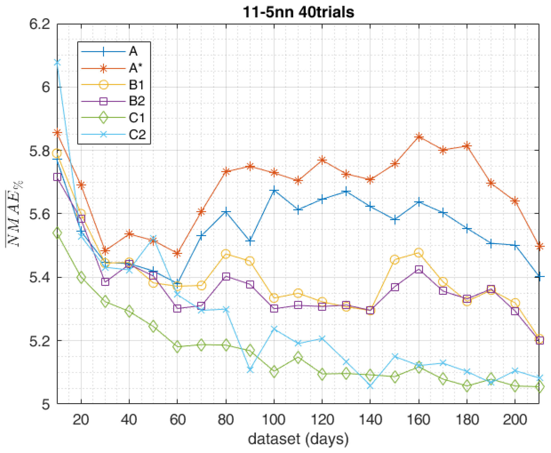
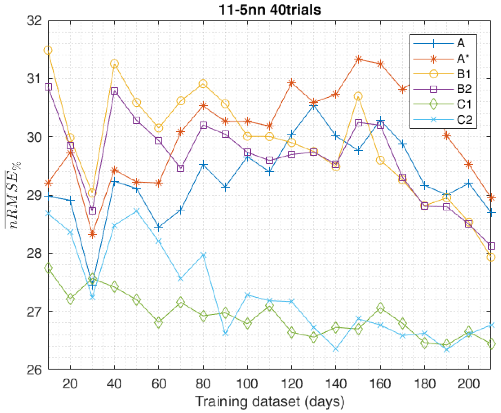
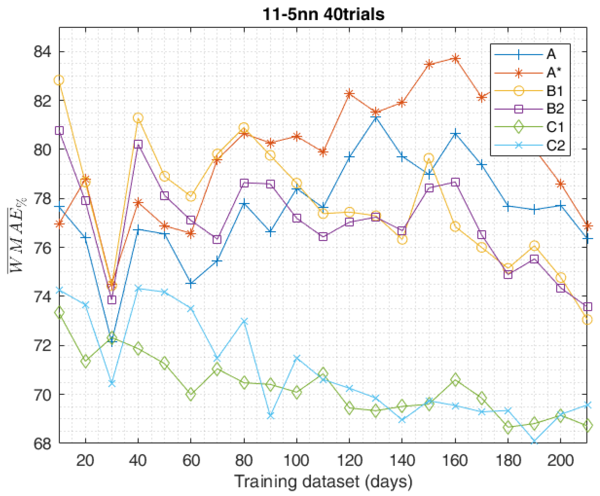
The study carried on so far aimed to compare different methods in the data-set composition employed for the training of the ANN, highlighting the most effective ones. The obtained results of the day-ahead forecasts were analysed by the indexes shown in Section 3 and led to the following results. The graph in Figure 15 shows the trend of the calculated for the methods in the training-set composition, according to increasing data-set sizes. The best training method, which globally performed better with all the data-sets considered, was undoubtedly C1. Instead, in the short-range training, with only 10 days available in the data-set, method C2 scored the worst result with equal to 6.079. In accordance with the increasing data-sets method, C2 aligned with C1 above 90–130 days. The same trends of the other evaluation indexes are equally shown in Figure 16, Figure 17 and Figure 18 and confirm the same results. From this perspective, method C2 scored the worst result, with equal to 36.51. According to the shown in Figure 15, methods B1 and B2 generally performed pretty much the same.
As a general comment on the reported results, it can be stated that method A is best suited when the availability of historical data is limited (e.g., newly deployed PV plant), while method C1 appears to be most effective in the case of a greater availability of data (e.g., at least one year of power measurements from the considered PV facility). Generally speaking, ensembles composed of independent trials are most effective. The performance of methods B1 and B2 was halfway between A and C, and their effectiveness in the case of newly deployed PV plants became significant after a minimum period of measurement data accumulation (above 60 days).
6. Conclusions
This paper has presented a specific study aimed to analyze the effect of different approaches in the composition of a training data-set for the day-ahead forecasting of PV power production. In particular, the authors proposed different procedures to set-up the training and validation data-sets for the ANN used in physical hybrid method to perform the power forecast in view of the electricity market. The here-outlined approaches can be adopted to set-up data-sets based on either historical data retrieved from an existing PV plant or on incremental data measurements in a newly deployed PV facility. In particular, the influence of different data-set compositions on the forecast outcome has been inspected by increasing the training dataset size and by varying the training and validation shares, in order to assess the most effective training method of this machine learning approach, based on commonly used and newly-defined performance indexes for the prediction error. The reported results have been validated over a 1-year time range of experimentally measured data from a real PV power plant, considering a comparison of various error measures and showing the best approach for the different cases of either newly deployed or already existing PV facilities.
Author Contributions
In this research activity, all of the authors were involved in the data analysis and preprocessing phase, the simulation, the results analysis and discussion, and the manuscript’s preparation. All of the authors have approved the submitted manuscript. All the authors equally contributed to the writing of the paper.
Conflicts of Interest
The authors declare no conflict of interest.
References
- Pelland, S.; Remund, J.; Kleissl, J.; Oozeki, T.; De Brabandere, K. Photovoltaic and solar forecasting: State of the art. IEA PVPS Task 2013, 14, 1–36. [Google Scholar]
- Paulescu, M.; Paulescu, E.; Gravila, P.; Badescu, V. Weather Modeling and Forecasting of PV Systems Operation; Springer Science & Business Media: Berlin, Germany, 2012. [Google Scholar]
- Raza, M.Q.; Nadarajah, M.; Ekanayake, C. On recent advances in PV output power forecast. Sol. Energy 2016, 136, 125–144. [Google Scholar] [CrossRef]
- Faranda, R.S.; Hafezi, H.; Leva, S.; Mussetta, M.; Ogliari, E. The Optimum PV Plant for a Given Solar DC/AC Converter. Energies 2015, 8, 4853–4870. [Google Scholar] [CrossRef] [Green Version]
- Dolara, A.; Lazaroiu, G.C.; Leva, S.; Manzolini, G.; Votta, L. Snail Trails and Cell Microcrack Impact on PV Module Maximum Power and Energy Production. IEEE J. Photovolt. 2016, 6, 1269–1277. [Google Scholar] [CrossRef]
- Omar, M.; Dolara, A.; Magistrati, G.; Mussetta, M.; Ogliari, E.; Viola, F. Day-ahead forecasting for photovoltaic power using artificial neural networks ensembles. In Proceedings of the 2016 IEEE International Conference on Renewable Energy Research and Applications (ICRERA), Birmingham, UK, 20–23 November 2016; pp. 1152–1157. [Google Scholar]
- Cali, Ü. Grid and Market Integration of Large-Scale Wind Farms Using Advanced Wind Power Forecasting: Technical and Energy Economic Aspects; Erneuerbare Energien und Energieeffizienz—Renewable Energies and Energy Efficiency; Kassel University Press: Kassel, Germany, 2011. [Google Scholar]
- Ni, Q.; Zhuang, S.; Sheng, H.; Kang, G.; Xiao, J. An ensemble prediction intervals approach for short-term PV power forecasting. Sol. Energy 2017, 155, 1072–1083. [Google Scholar] [CrossRef]
- Simonov, M.; Mussetta, M.; Grimaccia, F.; Leva, S.; Zich, R. Artificial intelligence forecast of PV plant production for integration in smart energy systems. Int. Rev. Electr. Eng. 2012, 7, 3454–3460. [Google Scholar]
- Duan, Q.; Shi, L.; Hu, B.; Duan, P.; Zhang, B. Power forecasting approach of PV plant based on similar time periods and Elman neural network. In Proceedings of the 2015 Chinese Automation Congress (CAC), Wuhan, China, 27–29 November 2015; pp. 1258–1262. [Google Scholar]
- Gardner, M.; Dorling, S. Artificial neural networks (the multilayer perceptron)—A review of applications in the atmospheric sciences. Atmos. Environ. 1998, 32, 2627–2636. [Google Scholar] [CrossRef]
- Nelson, M.; Illingworth, W. A Practical Guide to Neural Nets; Physical Sciences; Addison-Wesley: Boston, MA, USA, 1991; 316p. [Google Scholar]
- Bose, B.K. Neural Network Applications in Power Electronics and Motor Drives—An Introduction and Perspective. IEEE Trans. Ind. Electron. 2007, 54, 14–33. [Google Scholar] [CrossRef]
- Ogliari, E.; Dolara, A.; Manzolini, G.; Leva, S. Physical and hybrid methods comparison for the day ahead PV output power forecast. Renew. Energy 2017, 113, 11–21. [Google Scholar] [CrossRef]
- Elder, J.F.; Abbott, D.W. A comparison of leading data mining tools. In Proceedings of the Fourth International Conference on Knowledge Discovery and Data Mining, New York, NY, USA, 27–31 August 1998; Volume 28. [Google Scholar]
- Bergstra, J.; Breuleux, O.; Bastien, F.; Lamblin, P.; Pascanu, R.; Desjardins, G.; Turian, J.; Warde-Farley, D.; Bengio, Y. Theano: A CPU and GPU math compiler in Python. In Proceedings of the 9th Python in Science Conference, Austin, TX, USA, 28 June–3 July 2010; pp. 1–7. [Google Scholar]
- Collobert, R.; Kavukcuoglu, K.; Farabet, C. Torch7: A matlab-like environment for machine learning. In Proceedings of the BigLearn, NIPS Workshop, Sierra Nevada, Spain, 16–17 December 2011. Number EPFL-CONF-192376. [Google Scholar]
- Kalogirou, S. Artificial Intelligence in Energy and Renewable Energy Systems; Nova Publishers: Hauppauge, NY, USA, 2007. [Google Scholar]
- Duffie, J.A.; Beckman, W.A. Solar Engineering of Thermal Processes; John Wiley & Sons: Hoboken, NJ, USA, 2013. [Google Scholar]
- Gandelli, A.; Grimaccia, F.; Leva, S.; Mussetta, M.; Ogliari, E. Hybrid model analysis and validation for PV energy production forecasting. In Proceedings of the 2014 International Joint Conference on Neural Networks (IJCNN), Beijing, China, 6–11 July 2014; pp. 1957–1962. [Google Scholar]
- Dolara, A.; Grimaccia, F.; Leva, S.; Mussetta, M.; Ogliari, E. A Physical Hybrid Artificial Neural Network for Short Term Forecasting of PV Plant Power Output. Energies 2015, 8, 1138–1153. [Google Scholar] [CrossRef] [Green Version]
- Rana, M.; Koprinska, I.; Agelidis, V.G. Forecasting solar power generated by grid connected PV systems using ensembles of neural networks. In Proceedings of the 2015 International Joint Conference on Neural Networks (IJCNN), Killarney, Ireland, 12–16 July 2015; pp. 1–8. [Google Scholar]
- Grimaccia, F.; Leva, S.; Mussetta, M.; Ogliari, E. ANN Sizing Procedure for the Day-Ahead Output Power Forecast of a PV Plant. Appl. Sci. 2017, 7, 622. [Google Scholar] [CrossRef]
- Netsanet, S.; Zhang, J.; Zheng, D.; Hui, M. Input parameters selection and accuracy enhancement techniques in PV forecasting using Artificial Neural Network. In Proceedings of the 2016 IEEE International Conference on Power and Renewable Energy (ICPRE), Shanghai, China, 21–23 October 2016; pp. 565–569. [Google Scholar]
- Panapakidis, I.P.; Christoforidis, G.C. A hybrid ANN/GA/ANFIS model for very short-term PV power forecasting. In Proceedings of the 2017 11th IEEE International Conference on Compatibility, Power Electronics and Power Engineering (CPE-POWERENG), Cadiz, Spain, 4–6 April 2017; pp. 412–417. [Google Scholar]
- Tetko, I.V.; Livingstone, D.J.; Luik, A.I. Neural network studies. 1. Comparison of overfitting and overtraining. J. Chem. Inf. Comput. Sci. 1995, 35, 826–833. [Google Scholar] [CrossRef]
- Hansen, L.K.; Salamon, P. Neural network ensembles. IEEE Trans. Pattern Anal. Mach. Intell. 1990, 12, 993–1001. [Google Scholar] [CrossRef]
- Perrone, M.P. General averaging results for convex optimization. In Proceedings of the 1993 Connectionist Models Summer School; Psychology Press: London, UK, 1994; pp. 364–371. [Google Scholar]
- Odom, M.D.; Sharda, R. A neural network model for bankruptcy prediction. In Proceedings of the 1990 IJCNN International Joint Conference on Neural Networks, San Diego, CA, USA, 17–21 June 1990; pp. 163–168. [Google Scholar]
- Hagan, M.T.; Demuth, H.B.; Beale, M.H. Neural Network Design; Campus Publishing Service, University of Colorado Bookstore: Boulder, CO, USA, 2014; ISBN 9780971732100. [Google Scholar]
- Chen, S.H.; Jakeman, A.J.; Norton, J.P. Artificial intelligence techniques: an introduction to their use for modelling environmental systems. Math. Comput. Simul. 2008, 78, 379–400. [Google Scholar] [CrossRef]
- Monteiro, C.; Fernandez-Jimenez, L.A.; Ramirez-Rosado, I.J.; Munoz-Jimenez, A.; Lara-Santillan, P.M. Short-Term Forecasting Models for Photovoltaic Plants: Analytical versus Soft-Computing Techniques. Math. Probl. Eng. 2013, 2013, 767284. [Google Scholar] [CrossRef]
- Ulbricht, R.; Fischer, U.; Lehner, W.; Donker, H. First Steps Towards a Systematical Optimized Strategy for Solar Energy Supply Forecasting. In Proceedings of the European Conference on Machine Learning and Principles and Practice of Knowledge Discovery in Databases (ECMLPKDD 2013), Riva del Garda, Italy, 23–27 September 2013. [Google Scholar]
- Kleissl, J. Solar Energy Forecasting and Resource Assessment; Academic Press: Cambridge, MA, USA, 2013. [Google Scholar]
- Ogliari, E.; Grimaccia, F.; Leva, S.; Mussetta, M. Hybrid Predictive Models for Accurate Forecasting in PV Systems. Energies 2013, 6, 1918–1929. [Google Scholar] [CrossRef] [Green Version]
- Wolfram, M.; Bokhari, H.; Westermann, D. Factor influence and correlation of short term demand for control reserve. In Proceedings of the 2015 IEEE Eindhoven PowerTech, Eindhoven, The Netherlands, 29 June–2 July 2015; pp. 1–5. [Google Scholar]
- SolarTechLab Department of Energy. Available online: http://www.solartech.polimi.it/ (accessed on 30 September 2017).
- ABB MICRO-0.25-I-OUTD. Available online: https://library.e.abb.com/public/0ac164c3b03678c085257cbd0061a446/MICRO-CDD_BCD.00373_EN.pdf (accessed on 21 January 2018).
- Leva, S.; Dolara, A.; Grimaccia, F.; Mussetta, M.; Ogliari, E. Analysis and validation of 24 hours ahead neural network forecasting of photovoltaic output power. Math. Comput. Simul. 2017, 131, 88–100. [Google Scholar] [CrossRef] [Green Version]
Figure 1.
Main features of the ANN training data-sets.

Figure 2.
Physical Hybrid Artificial Neural Network (PHANN) method schematic diagram.

Figure 3.
Hourly samples are progressively available in an incremental training database. PV: photovoltaic.
Figure 3.
Hourly samples are progressively available in an incremental training database. PV: photovoltaic.

Figure 4.
Training database composition for methods A, A*, and B.

Figure 5.
Hourly samples belonging to an extended period of time are available in a complete training database.
Figure 5.
Hourly samples belonging to an extended period of time are available in a complete training database.

Figure 6.
Hourly samples belonging to an extended period of time in a complete training database are randomly mixed.
Figure 6.
Hourly samples belonging to an extended period of time in a complete training database are randomly mixed.

Figure 7.
Example of the daily errors trend. : normalized mean absolute error; : normalized root mean square error; : weighted mean absolute error.
Figure 7.
Example of the daily errors trend. : normalized mean absolute error; : normalized root mean square error; : weighted mean absolute error.

Figure 8.
Normalized daily errors correlated in a scatterplot.

Figure 9.
Example of a sunny day forecast—1 April 2014—with the relevant evaluation indexes. : envelope-weighted mean absolute error.
Figure 9.
Example of a sunny day forecast—1 April 2014—with the relevant evaluation indexes. : envelope-weighted mean absolute error.

Figure 10.
Example of a cloudy day forecast—4 November 2014—with the relevant evaluation indexes.

Figure 11.
as a function of the dataset size.

Figure 12.
as a function of the dataset size.

Figure 13.
as a function of the dataset size.

Figure 14.
as a function of the dataset size.

Figure 15.
as a function of the dataset size.

Figure 16.
as a function of the dataset size.

Figure 17.
as a function of the dataset size.

Figure 18.
as a function of the dataset size.


Table 1.
Different methods for the composition of the ANN training data-sets which have been analysed. (90% 10%) = training set; = validation set.
Table 1.
Different methods for the composition of the ANN training data-sets which have been analysed. (90% 10%) = training set; = validation set.
| Method | Data-Set | Trials | Samples |
|---|---|---|---|
| A | Incremental | Dependent | Consecutive (10% 90%) |
| A* | Incremental | Dependent | Consecutive (90% 10%) |
| B1 | Incremental | Independent | Random |
| B2 | Incremental | Dependent | Random |
| C1 | Complete | Independent | Random |
| C2 | Complete | Dependent | Random |
© 2018 by the authors. Licensee MDPI, Basel, Switzerland. This article is an open access article distributed under the terms and conditions of the Creative Commons Attribution (CC BY) license (http://creativecommons.org/licenses/by/4.0/).
Share and Cite
MDPI and ACS Style
Dolara, A.; Grimaccia, F.; Leva, S.; Mussetta, M.; Ogliari, E. Comparison of Training Approaches for Photovoltaic Forecasts by Means of Machine Learning. Appl. Sci. 2018, 8, 228. https://0-doi-org.brum.beds.ac.uk/10.3390/app8020228
AMA Style
Dolara A, Grimaccia F, Leva S, Mussetta M, Ogliari E. Comparison of Training Approaches for Photovoltaic Forecasts by Means of Machine Learning. Applied Sciences. 2018; 8(2):228. https://0-doi-org.brum.beds.ac.uk/10.3390/app8020228
Chicago/Turabian StyleDolara, Alberto, Francesco Grimaccia, Sonia Leva, Marco Mussetta, and Emanuele Ogliari. 2018. "Comparison of Training Approaches for Photovoltaic Forecasts by Means of Machine Learning" Applied Sciences 8, no. 2: 228. https://0-doi-org.brum.beds.ac.uk/10.3390/app8020228
Note that from the first issue of 2016, this journal uses article numbers instead of page numbers. See further details here.