Numerical Investigation into Effects of Viscous Flux Vectors on Hydrofoil Cavitation Flow and Its Radiated Flow Noise


School of Mechanical Engineering, Pusan National University, Busan 46241, Korea
*
Author to whom correspondence should be addressed.
Appl. Sci. 2018, 8(2), 289; https://0-doi-org.brum.beds.ac.uk/10.3390/app8020289
Submission received: 27 November 2017
/
Revised: 26 January 2018
/
Accepted: 11 February 2018
/
Published: 15 February 2018
(This article belongs to the Special Issue Underwater Acoustics, Communications and Information Processing)
Abstract
:In this study, cavitation flow around a hydrofoil and its radiated hydro-acoustic fields were numerically investigated, with an emphasis on the effects of viscous flux vectors. The full three-dimensional unsteady compressible Reynolds-averaged Navier–Stokes equations were numerically solved. The mass transfer model was adopted to model phase changes between liquid water and vapor. To resolve the numerical instability problem arising from the rapid changes in local density and speed of sound of the mixture, the preconditioning and dual-time stepping methods were employed. The filter-based turbulent model was applied to resolve the unstable cavitation flow field more accurately. In splitting the viscous terms, three approaches for dealing with viscous flux vectors were considered: the so-called viscous lagging, full viscous, and thin-layer models. Radiated hydro-acoustic waves were predicted by applying the Ffowcs Williams and Hawkings equations. The effects of the viscous flux vectors on the predicted flow fields and its radiated noise were then examined by comparing the hydro-dynamic forces, velocity distribution, volume fraction, far-field sound directivities, and sound spectrum of the three approaches. The results revealed that the thin-layer model can provide predictions as accurate as the full viscous model, but required less computational time.
1. Introduction
Cavitation typically occurs when the local pressure in a flow field drops below the vapor pressure of the liquid, and forms vapor cavities or gas bubbles. The generation, development, and extinction of cavitation involves subsequent pressure fluctuations, causing damage to neighboring bodies, and hydro-acoustic flow noise problems. Therefore, numerous experimental and numerical studies have been conducted to investigate the cavitation phenomena.
Experimental studies were typically conducted using scale models in water-tunnels, with high-speed cameras used to visualize the cavitation with high-speed image processing techniques. Shen and Dimotakis [1], Kawanami et al. [2], and Wang et al. [3] experimentally investigated cavitating flow around submerged hydrofoils. Park et al. [4] proposed noise source localization techniques for rotating propellers, by using source strength estimation methods in swallow water conditions. Kopriva et al. [5] and Karn et al. [6] studied the dynamics of ventilated cavitation with steady and periodic gust flows. However, the experimental approaches, based on scale models, typically suffer from an inability to apply the scaled results to the full-scale objects because of numerous non-dimensional parameters.
As an alternative approach, numerical methods have been developed and used to investigate the cavitation phenomena. Merkle et al. [7] and Singhal et al. [8] proposed mass transfer models (also known as cavitation models) to deal with phase changes between liquid and vapor. Kunz et al. [9], Huang [10], Esfahanian and Akbarzadeh [11], and Ha and Park [12] proposed preconditioning methods to resolve numerical instability issues, that arise from large disparities between the acoustic and convective wave speeds. Johansen et al. [13] developed a filter-based turbulence model that was applied across a wide range of multi-phase problems [14,15,16].
However, as cavitation is highly unstable and sensitive to turbulent flow, it remains difficult to resolve the detailed features and mechanisms. To improve the understanding of the cavitation phenomena, the relevant numerical and physical issues need to be quantified. In addition, the International Maritime Organization (IMO) recently adopted guidelines to reduce underwater noise from commercial ships, recognizing that underwater-radiated noise from commercial ships has adverse effects on marine lift. This fact and the understanding that the propeller cavitation is one of most contributing factors to flow noise sources of commercial ships necessitates the improved understanding of numerical and physical issues related to cavitation flows and its radiated noise. For this purpose, in this study, the effects of viscous flux vectors on the generation, development, and extinction of cavitation from a hydrofoil, and the radiated hydro-acoustic flow noise, is numerically investigated with three different approaches to treating viscous flux vectors: viscous lagging, thin-layer, and full viscous models. Numerous numerical studies for cavitation phenomena can be classified into these three approaches. However, the effects of viscous flux vectors are not made clear. To reveal the effects of viscous flux vectors on the cavitation phenomena, the flow fields are predicted by solving the full three-dimensional (3D) unsteady compressible Reynolds-averaged Navier–Stokes (RANS) equations. The governing equations are numerically solved using the preconditioned implicit pseudo-time marching scheme, combined with the filter-based turbulence models. The homogeneous mixture model is applied to model the multi-phase fluid. When the phase of fluid is changed from water vapor to liquid water and vice versa, mass transfer is involved and its effects can be modelled with mass transfer models, also known as cavitation models. In this study, to model these phenomena, Merkle’s cavitation model [7] is applied. Based on the flow field results, radiated hydro-acoustic fields are predicted using the Ffowcs Williams and Hawkings (FW-H) equation. The effects of viscous flux vectors on the cavitation flows and the associated acoustic fields, are investigated in terms of cavity structures, volume fractions, velocity distribution, acoustic pressure spectrum, and directivities.
In Section 2, the problem is described using computational grids and boundary conditions. In Section 3, the governing equations and the numerical methods are described, with detailed explanations concerning the treatment of viscous flux vectors in association with the preconditioned implicit pseudo-time marching scheme. In Section 4, the numerical methods used in this study are validated. The predicted results of the cavitation flow field and its radiated acoustic field are then presented and analyzed, with emphasis placed on the effects of viscous flux vectors according to the types of viscous flux models employed.
2. Target Problem Description
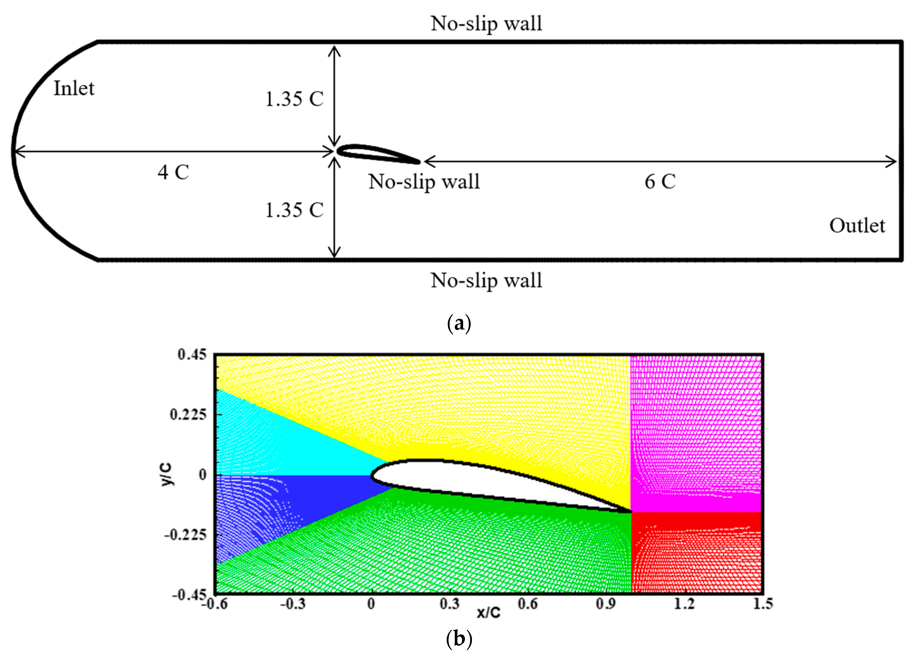
The Clark-Y hydrofoil was selected as the target hydrofoil as the referenced flow conditions and the associated flow data have been reported on in previous experimental studies by Kawanami et al. [2] and Wang et al. [3] and summarized in Table 1. The target hydrofoil, with a chord length, C, of 0.07 m, is subject to an inflow velocity, , where , at an angle of attack . The chord-length-based Reynolds number, , and the cavitation number, σ, is 0.8. Figure 1 shows the computational domain and the grids used in this study. The domain has a rectangular cross-section of 2.70 C (H) × 1.0 C (W) and the distance between the inlet and the leading edge of the hydrofoil is 4 C. The constant inlet velocity and the outlet static pressure specified in the referenced experimental data, are applied on the inlet and outlet boundaries, respectively. The other variables at the boundaries are extrapolated from the interior grids. The no-slip wall boundary condition is applied on both the hydrofoil surface and the water-tunnel wall. To resolve the complex flow region near the hydrofoil surface more accurately, the grids near the hydrofoil are clustered to satisfy . The entire computation domain is divided into several blocks, on which the parallel computations are carried out using the message passing interface (MPI) library.
3. Governing Equations and Numerical Implementations
3.1. Governing Equations
The numerical analysis is implemented by solving the full three-dimensional unsteady compressible RANS equations with homogeneous mixture approach. The accurate and effective numerical simulation of a multi-phase problem is challenging, as numerical instability issues arise from the large variations in the speed of sound with rapid local density changes [9,11,12,16,17,18,19]. To resolve these problems, the preconditioned and dual-time stepping numerical methods are employed. The governing equation in a generalized curvilinear coordinate is expressed as follows
where is the vector of primitive variables; , , , , and are the convective and viscous flux vectors; is the source vector; and are the flux Jacobian matrix and the preconditioning matrix, respectively; and τ denote the physical and pseudo times, respectively.
These vectors are written as follows
where, the subscription x, y and z denote the Cartesian coordinates , and J is the Jacobian with the metrics of , , , , , , , , , which transform the coordinates from the Cartesian coordinates to the generalized curvilinear coordinates . is the static pressure, is the density, g is the acceleration. u, v, w, U, V and W are the velocity components in the x, y, z, , and directions, respectively. is the tensor of the viscous stress. is the heat flux. is the total enthalpy.
In this study, to model the multi-phase fluid, the homogeneous mixture approach is applied. The homogeneous mixture approach assumed the fluids to exist in mixed-phase state which means each phase shares the pressure, velocity and temperature under the assumption of mechanical and thermo-dynamical equilibrium. Thus, only a pair of moment equations for mixture phase is required. The phase of fluid can be represented by mass fraction and volume fraction with the following relations.
where, subscription l, v, g and m represent the phase of fluids; liquid water, water vapor, non-condensable gases and mixture, respectively.
With the relation of Equation (3), total mass and volume fraction is conserved within flow field. If or is equal to 1, the fluid exists in pure liquid water, and if or is equal to 1, the fluid exists in pure water vapor. Note that, the non-condensable gas terms are added to model the artificial ventilation. However, in this study, any ventilation is not considered. Therefore, or is always set to 0.
The phase change between water vapor and liquid water is modelled by adding mass transfer terms to the source. The two terms of and in represent the mass transfer from water vapor to liquid water (condensation) and vice versa (evaporation). In this study, these phase change phenomena are considered by applying Merkle’s cavitation model [7] in the form
where, is vapor pressure of liquid, and are empirical coefficients, is the characteristic time scale which defined as . The empirical coefficients are set to the recommended [7] value of and .
The fundamental hypothesis of the Merkle’s model is that the cavitation phenomena are occurred only due to the difference between the local static pressure, , and vapor pressure of liquid, . If the local static pressure decreases below the vapor pressure, evaporation occurs and thus the phase of fluid is changed from liquid water to water vapor with the amount of mass transfer rate of . In contrast, if the local static pressure increases above the vapor pressure, the reversal phenomena occur with the amount of mass transfer rate of .
To close the system, the equation of state (EOS) for the liquid water, water vapor and mixture are required. In this study, the properties such as density, enthalpy, dynamic viscosity and thermal conductivity of liquid water, water vapor, mixture and its derivatives are considered as the function of pressure and temperature as reported by international standard IAPWS-IF97 [20].
3.2. Turbulence Modeling
In this study, the low Reynolds number k-ε turbulence model by Jones and Launder [21,22] is used to simulate turbulent flows. Based on the results from a previous study [16], the filter-based turbulent viscosity modification proposed by Johansen et al. [13] is adopted to predict unstable cavitation flows more accurately. The transport equations of the low Reynolds number k-ε turbulence model, and the modified turbulent viscosity, are written as follows
where is the turbulence production term; and are the dissipation terms; , , and are functions of the Reynolds number; and , , , , and are empirical coefficients.
3.3. Numerical Implementations
As the RANS equations are non-linear, a linearization process is essential. In this study, the governing equations are linearized implicitly. For the physical and pseudo time-derivative terms, the 2nd and 1st order backward differences are applied, respectively, in the following form
The flux terms are linearized by using a Taylor series expansion. As the convective fluxes are only a function of primitive variables, if there is no grid-motion, the linearization process is simply achieved as follows
where , and are the convective flux Jacobian matrices.
The viscous fluxes are a function of the primitive variables, gradients of the primitive variables, and their multiples. Therefore, additional terms appear in a linearization process for viscous fluxes as follows
where , and are the viscous flux Jacobian matrices.
After substituting Equations (7)–(9) into Equation (1), the governing equations can be written as
On the left-hand side, the additional linearization of the terms , and , by is required to construct the matrix equation for the dependent variables. The chain rule is used for the linearization as follows
After substituting Equation (11) into the second term of the left-hand side of Equation (10), it can be rewritten as
As a result, Equation (12) now includes the mixed derivatives terms, such as and , that distort the diagonal matrix form. According to Hoffmann and Chiang [23], omitting these terms does not affect the accuracy of the solutions. Thus, in this study, these terms are neglected. Equation (12) then can be written as
In addition, if the fluid obeys the Stokes’ hypothesis and the transport coefficients, such as μ, κ, and λ are locally constant, i.e., slowly change with respect to temperature variations, Equation (13) can be reduced to the following form [24,25,26].
Similar processes can be applied to the viscous flux terms in the η- and ζ-directions. The final form of the governing equation can then be expressed as follows
Equation (15) is solved numerically implicitly, using the alternating direction implicit algorithm. The temporal derivative terms of the physical and pseudo times are discretized using the 2nd and 1st order backward differences, respectively. The monotonic upstream-centered scheme for conservation laws (MUSCL), and the 2nd order central difference schemes, are applied to the convective and viscous flux terms, respectively. For more detailed descriptions of the numerical methodologies, except for the additional linearization terms of the viscous flux that are the main subject of this study, the studies conducted by Ha and Park [12] and Kim et al. [16] can be referred to.
3.4. Viscous Flux Treatements
In this study, to investigate the effects of viscous fluxes on cavitation flow and the radiated acoustic field, three different approaches are presented: viscous lagging, full viscous, and thin-layer approximations.
3.4.1. Viscous Lagging Approach
The viscous lagging method, the simplest model, is discussed here. This method excludes the viscous flux terms from the implicit part. Therefore, the viscous terms are only considered explicitly in the pseudo time. Equation (15) can then be rewritten in the form
3.4.2. Full Viscous Approach
As the most accurate model, the full viscous approach comprises all the stream-wise (ξ), circumferential (ζ), and normal (η) viscous flux terms. The resultant governing equation is as per Equation (15). Similar approaches have been employed in numerous previous studies on cavitation flows. Granier et al. [28] applied the incompressible scheme to a flat-plate flow, a lid-driven cavity flow, and the impingement of a liquid drop on a solid wall. Senocak and Shyy [29] developed a pressure-based compressible solver and applied it to cavitation flow over hemispherical and blunt bodies. Based on the prediction results, some of the empirical constants of the standard k-ε turbulent model were modified to predict recirculation zones more accurately. Owis and Nayfeh [19] also tested three-dimensional incompressible multi-phase solvers on natural and ventilated cavitation flows, over axisymmetric bodies with hemispherical and blunt head forms, by varying computational conditions, such as cavitation number and angle of attack.
3.4.3. Thin-Layer Approximation
As a compromise model between the accuracy and efficiency of numerical methods, thin-layer approximation is considered. When the flow separation is not significant, or the normal gradient of the stress terms is significantly greater than the stream-wise and circumferential gradients, the thin-layer approximation can be used [22,30,31]. This approach neglects stream-wise (ξ) and circumferential (ζ) viscous terms, and thus only considers normal (η) viscous fluxes. The governing equation for thin-layer approximation is then reduced as
Kunz et al. [9] applied a thin-layer approximation to the prediction of axisymmetric and three-dimensional cavitation flows for several configurations. Although some of the results were compared to measured data, the accuracy and efficiency were not analyzed in detail, specifically with regard to the full viscous approach, one of main goals in this study.
3.5. Acoustic Analogy for Cavitation Noise Prediction
Based on cavitation flow fields predicted using each of the above three viscous treatment approaches, the radiated cavitation noise from a hydrofoil is predicted by the FW-H equation [32]. In this study, so-called hybrid techniques to predict hydro-acoustic pressure waves are employed [33,34,35,36]. The hybrid techniques consist of three steps; (1) flow field predictions by solving full 3D compressible RANS equations; (2) hydro-acoustic source modelling from the flow field results based on FW-H equation; and (3) linear wave propagation. Note that the present hybrid method does not consider the scattering and refraction of acoustic waves due to changes in sound velocity of media between source and acoustic regions. Therefore, the predicted hydro-acoustic fields are only used to investigate the relative contributions of the flow noise sources to the radiated acoustic field with emphasis on the role of cavitation flow characteristics due to viscous flux vectors.
The wave equation, that accounts for aerodynamic noise sources, was formulated for the first time by Lighthill, who attempted to find the origin of jet noise. Lighthill rearranged the Navier–Stokes equations into a wave equation with quadrupole source terms that were related to turbulent velocity fluctuations [37,38]. Curle [39] expanded Lighthill’s acoustic analogy to include the effects of stationary solid bodies in flow and found the dipole source term that accounts for the fluid loadings on body surfaces. Finally, Ffowcs Williams and Hawkings considered the effects of arbitrarily moving solid bodies and showed that these effects could be modeled by using the monopole and dipole source terms, including the Doppler effect. The integral form of the FW-H equation is written as follows
where r is distance between receiver and source, is the relative Mach number, and is a stress tensor defined as , where is static pressure, is the Kronecker delta, and is a viscous stress tensor. Lighthill’s stress tensor, , is defined as .
By following the procedure from a previous study (Kim et al. [16]), the FW-H equation can be rewritten in a form appropriate to account for flow noise, due to cavitation flow, over an acoustically compact stationary body, as follows
where is the vapor volume fraction.
The first term on the right-hand side of Equation (19) is the acoustic pressure due to the monopole source, caused by the rate of cavitation volume changes, and the second term is the dipole source of hydro-dynamic forces on the body surface.
4. Results and Discussion
4.1. Verification Tests
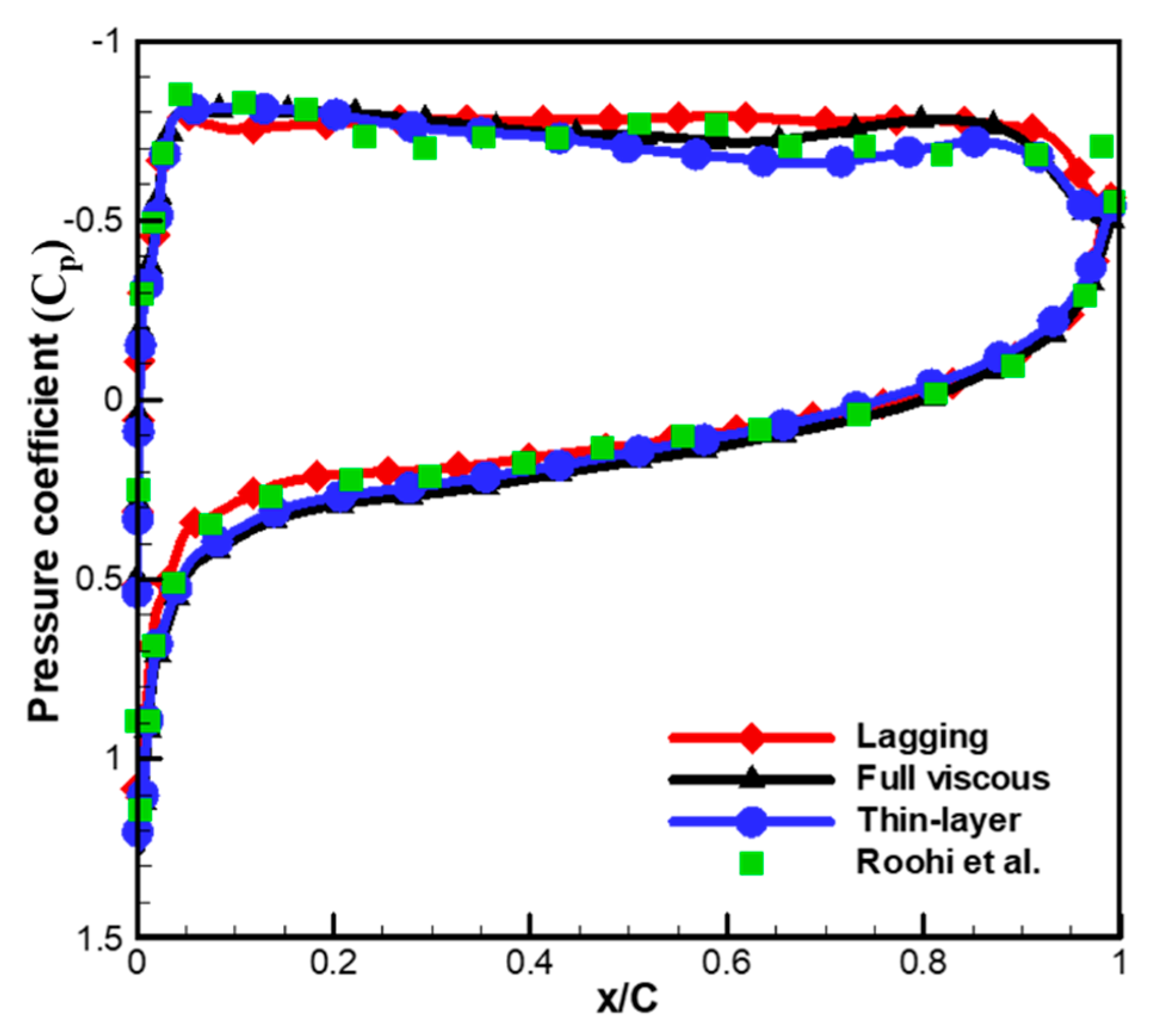
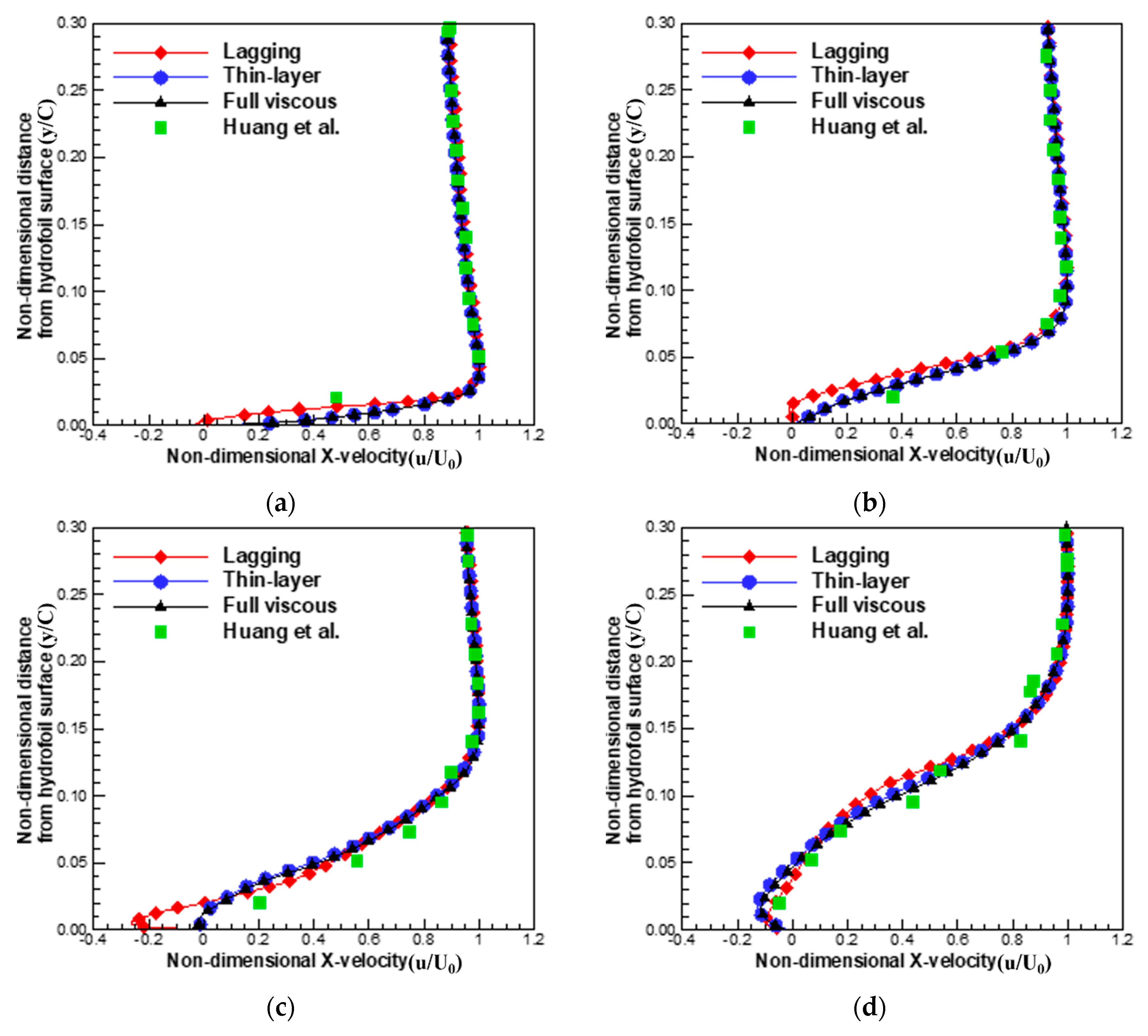
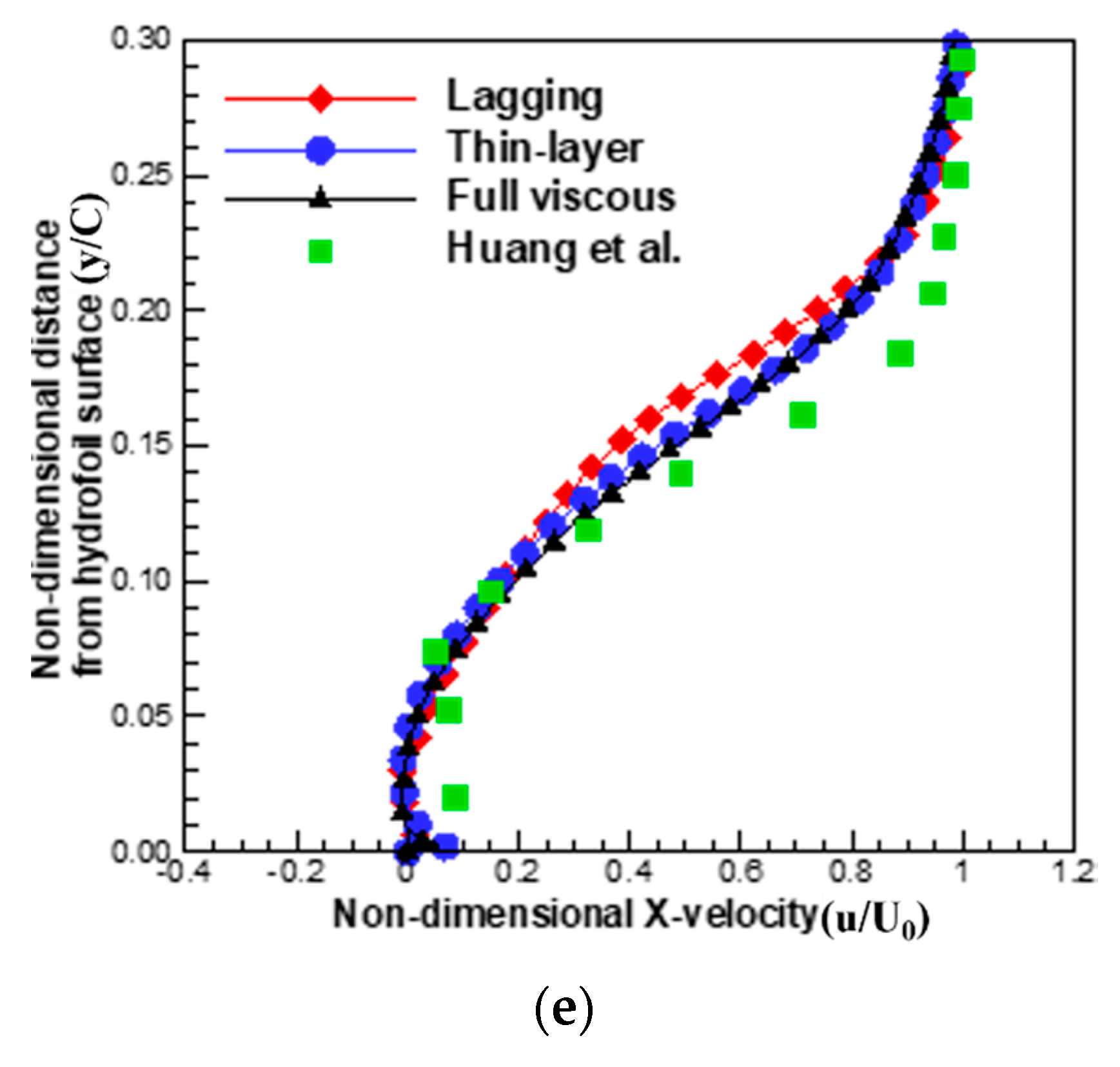
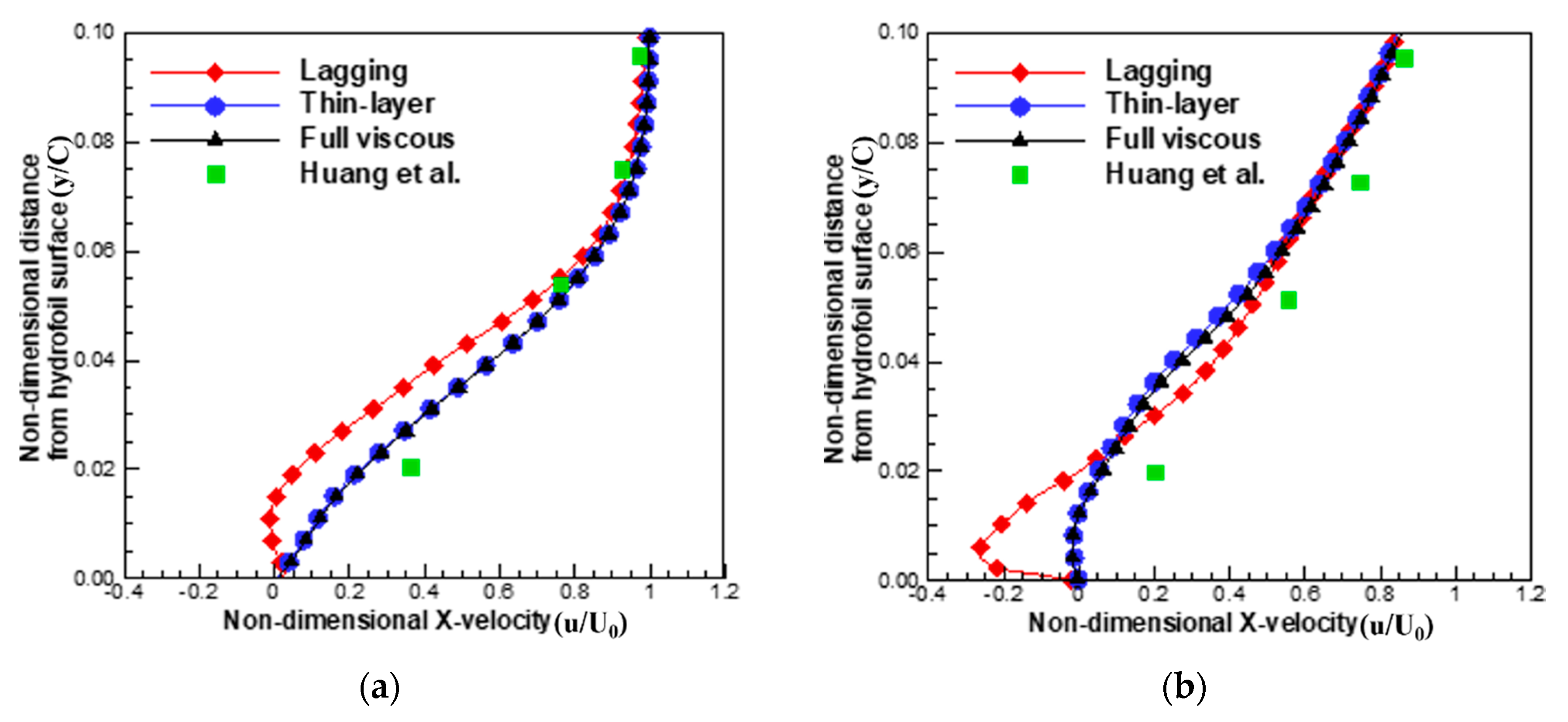
Prior to the detailed investigation of the predicted unsteady cavitation flows around the hydrofoil using the above viscous flux models, the averaged properties of the predicted flow field, using current numerical methods, are compared to the numerical results obtained from the large eddy simulation (LES) and experiments, to confirm the validity of the current numerical methods. Figure 2 compares the distribution of pressure coefficients over the hydrofoil surface with that of Roohi et al. [40], and Figure 3 compares the normal directional distributions of x-velocity from hydrofoil surface with that of Huang et al. [41]. As can be seen in those figures, there are good correlations between the three different approaches, as well as between the current results and the referred data. This result could imply that the viscous models do not have a significant effect on the averaged flow field, especially between the thin layer and the full viscous models.
4.2. Viscous Effects on Flow Field Prediction
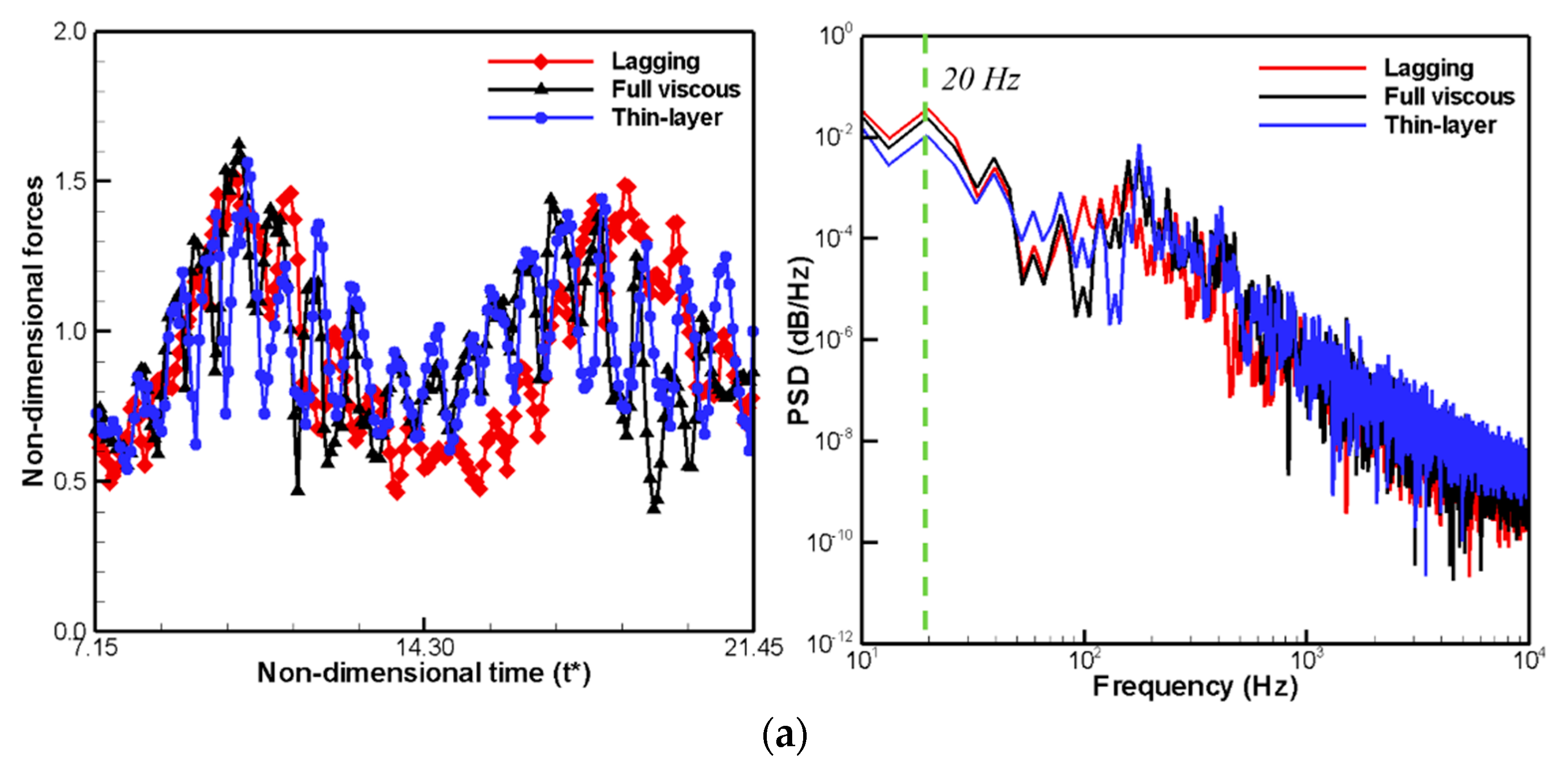
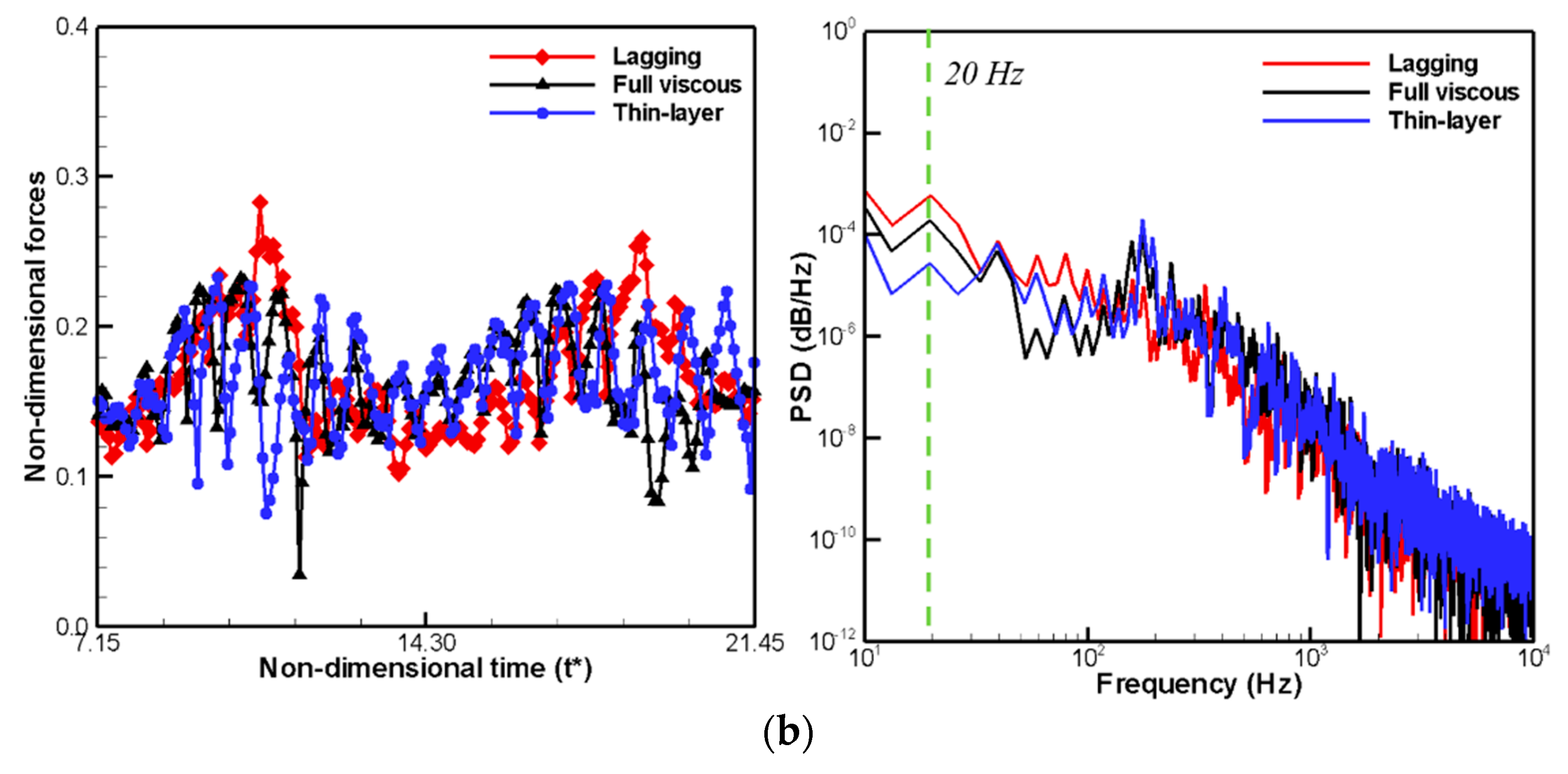
The effects of viscous fluxes, according to their approximate levels of predicting the generation, development, and extinction of cavitation over the hydrofoil, are investigated in terms of hydro-dynamic loadings, liquid volume fraction, and stream-wise velocity. First, the cyclic behavior of the generation, development, and extinction of cavitation needs to be identified. According to the experimental observations of Wang et al. [3], the current problem shows periodic behavior in terms of cavitation distribution over the hydrofoil, and a period (T) of 50 ms, i.e., with a fundamental frequency of 20 Hz. Figure 4 shows the time-histories of the predicted lift and drag coefficients, and the corresponding power spectral densities (PSD). As can be seen in the spectrums, the predicted results exhibit the same cycles in terms of unsteady loadings, irrespective of the viscous model adopted. Therefore, all subsequent comparisons between the different viscous models are performed during this cyclic period. Note that when the acoustic analogy is applied for the prediction of far-field noise under the assumption of compact sources, these unsteady loadings are used directly as the dipole source terms for flow noise. There is good correlation between the thin layer and the full viscous models, especially in terms of broadband components.
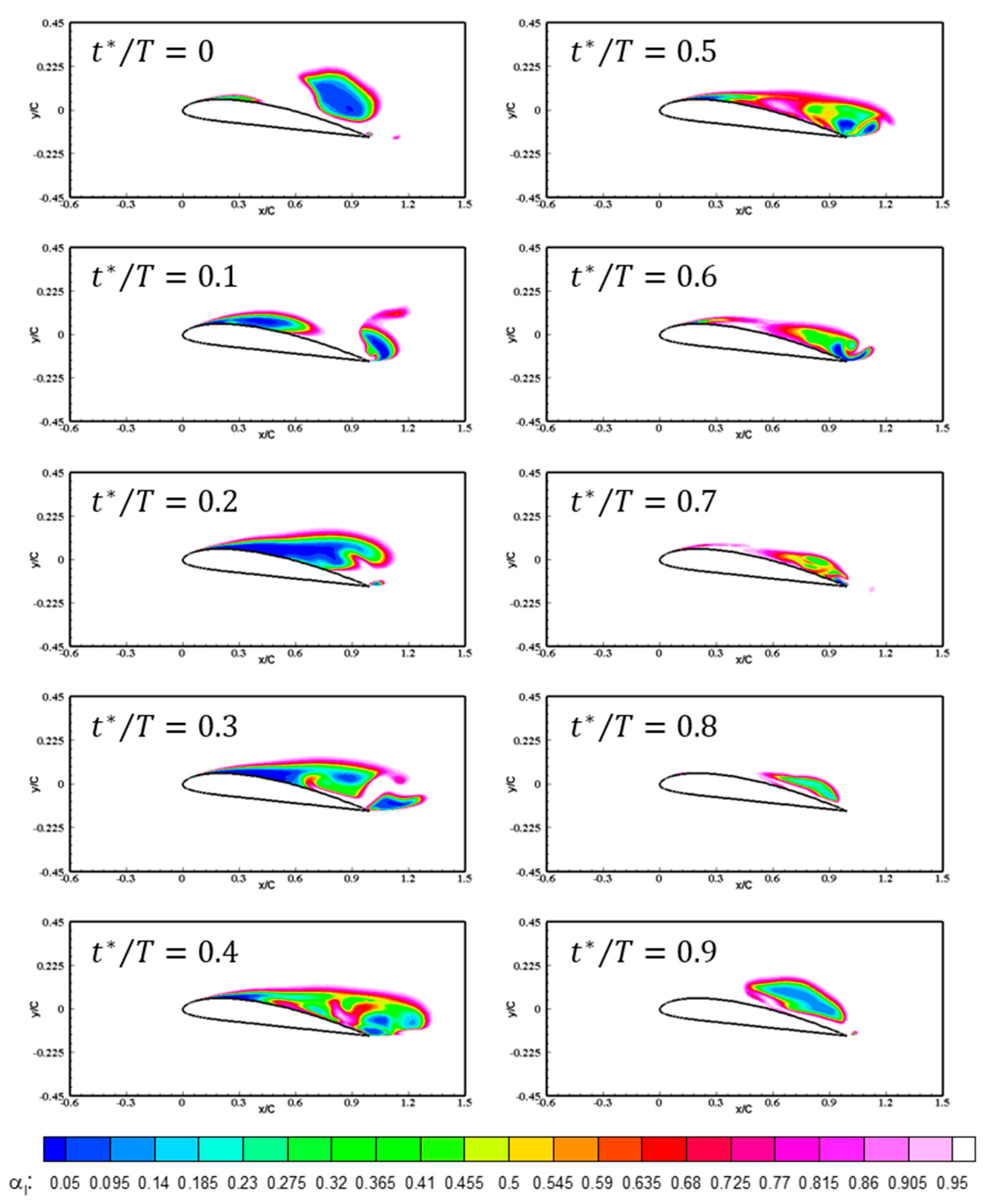
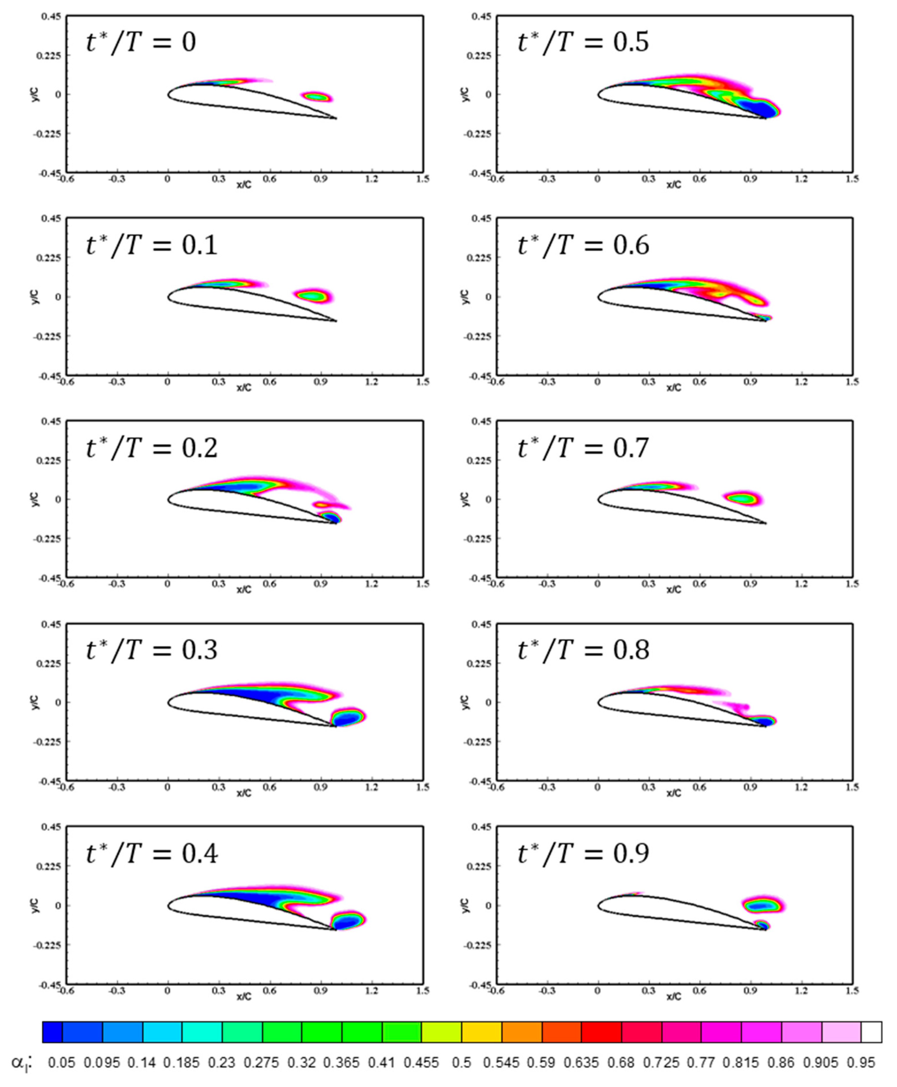
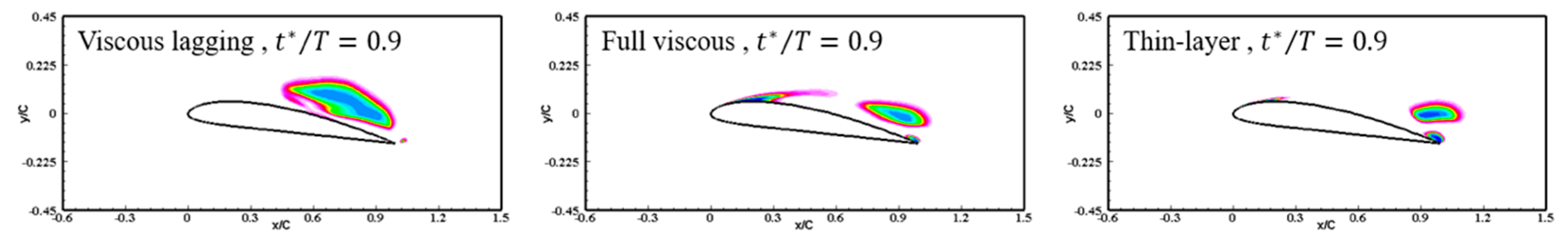
Figure 5 represents the predicted time-variation of total cavity volume and Figure 6, Figure 7 and Figure 8 compare the iso-contours of the predicted distributions of the liquid volume fractions of the three different viscous models, during a single cycle. All three cases exhibit similar cyclic behavior, comprising three phases: generation, development, and extinction of cavitation. At the beginning of the cycle, the cavities are generated from the leading edge, and extend rapidly toward the trailing edge. At the end of development, the fully extended cavities cover the entire suction side of the hydrofoil. At this point, the maximum cavity length is observed. After this fully developed instant, the cavities break into two at mid-chord. On the front side of the hydrofoil, the attached cavities continuously weaken toward the leading edge, while, on the other side, the cavities are rolled-up near the trailing edge and shed in a downstream direction. Although the three cases show similar cyclic behavior in terms of cavitation flow patterns, the detailed cavitation structures differ. In the case of the viscous lagging approach, it developed at , and then split at . However, the cavity structures in the thin-layer and full viscous cases developed relatively slowly between , and the fully developed cavities split at approximately . In addition, the thin-layer approach exhibited a quicker dissipation process of shedding cavities between .
Additionally, the cavitation distribution at the moment of minimum cavitation size also differs. Figure 9 compares the instantaneous cavity structures at the minimum developing moment () in viscous lagging, full viscous and thin-layer cases. At this instant, the experimental data by Wang et al. [3] shows that the cavities begin developing from the leading edge, and reach . In the trailing edge region, small attached cavities are observed. However, the viscous lagging model results show a significantly different pattern where, around the leading edge, no cavities have developed, and, in the trailing edge region, a large cavity is observed. For the thin-layer approach, the development of leading edge cavities is under-predicted, and they develop to approximately . The full viscous approach exhibits cavitation structures most similar to the experimental data, although the tail of the leading-edge cavities is slightly detached. However, the thin-layer and full viscous models exhibit similar patterns in terms of overall cavity structure.
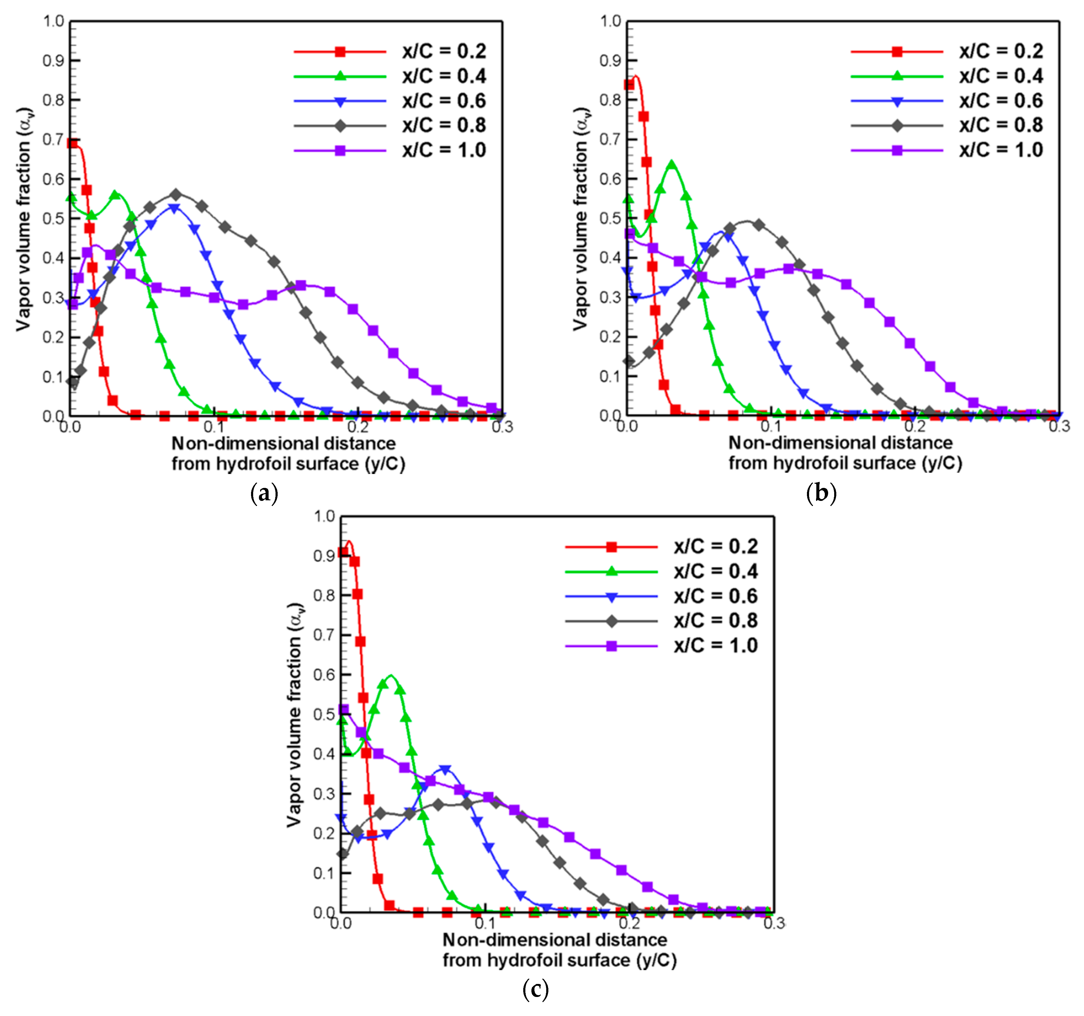
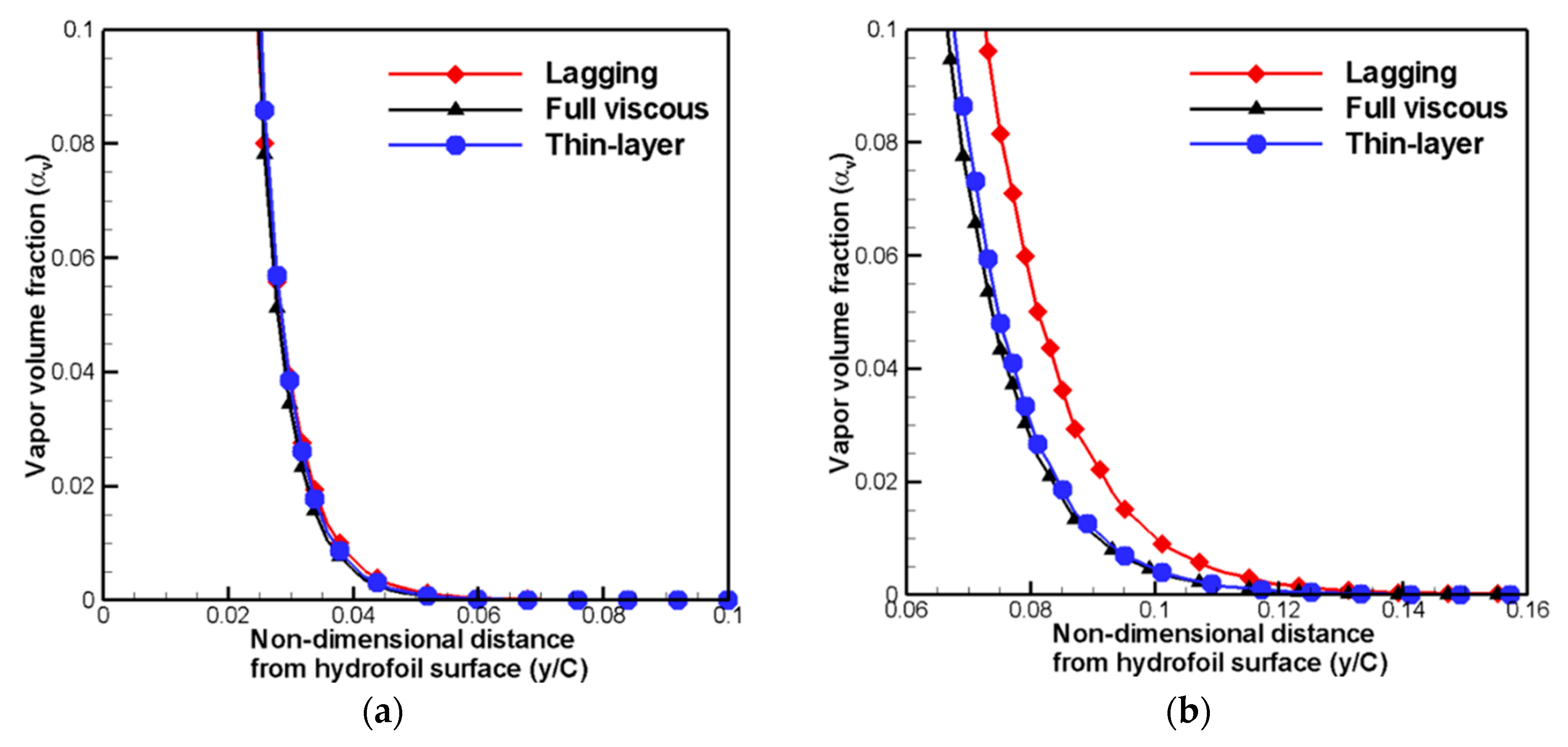
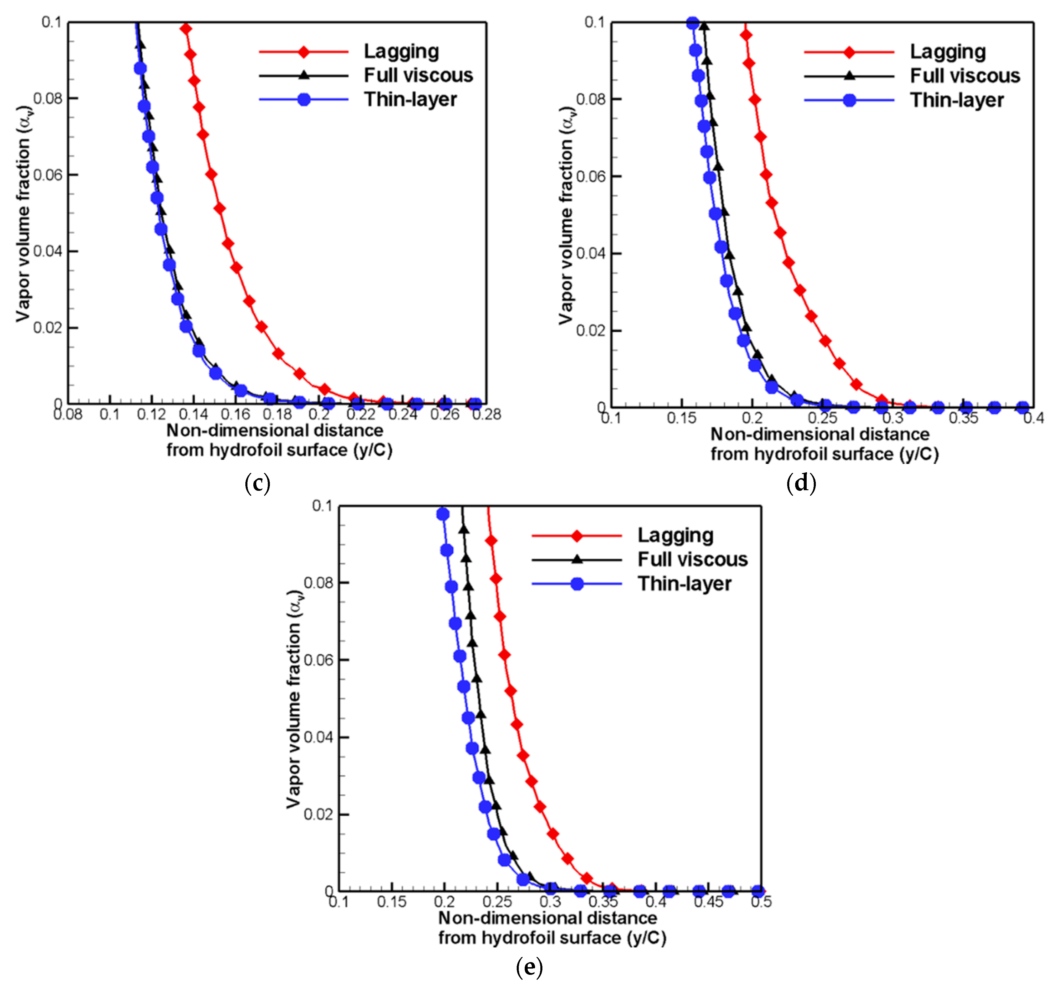
Figure 10 represent the comparison of time-averaged vapor volume fraction distribution at five different stream-wise locations for three different viscous flux vector treatment methods. As shown in Figure 10, most of cavity structures are developed near the hydrofoil surfaces, and above the there exist no cavities. When the homogeneous mixture approach is applied, the fluid existed in mixture phase. Therefore, it is hard to distinguish the boundary between liquid water and water vapor. Usually, the range of vapor volume fraction of is considered as water vapor phase. Therefore, the locations where the vapor volume fraction, , is equal to 0.05 can be as the boundary of developed cavity. Furthermore, the corresponding values of distance from the hydrofoil surface to the values of can be as the developed cavity thickness. Based on these points of view, to examine the effects of viscous flux vector treatment methods on developed cavity distributions and thickness in detail, zoomed vapor volume fraction distribution is compared as shown in Figure 11. The viscous lagging approach shows different results of vapor volume fraction distributions compared to the full viscous method and thin-layer approximation, except for the location of x/C = 0.2. Because complex flow phenomena such as separation did not occur at the leading edge, the effects of viscous flux vectors are relatively weak in this location. On the other hand, the full viscous method and thin-layer approximation show almost the same results for the location below the x/C = 0.6. For the locations of x/C = 0.8 and x/C = 1.0, thin-layer approximation shows a little lower values of cavity thickness.
Table 2 represents the predicted time-averaged cavity thickness of three viscous flux vector treatment methods at the different stream-wise locations with experimental results by Wang et al. [3]. Note that, in these results, the cavity thickness is nondimensionalized by chord length. As shown in Table 2, the viscous lagging approach shows the largest differences compared to experimental results at all of five different locations. On the other hand, the full viscous method and thin-layer approximation show good agreement with experimental results, except for the location of x/C = 0.2. Both of these methods show a little over-predicted result at x/C = 0.4 and x/C = 0.6, whereas a little under-predicted result at the locations of x/C = 0.8 and x/C = 1.0.
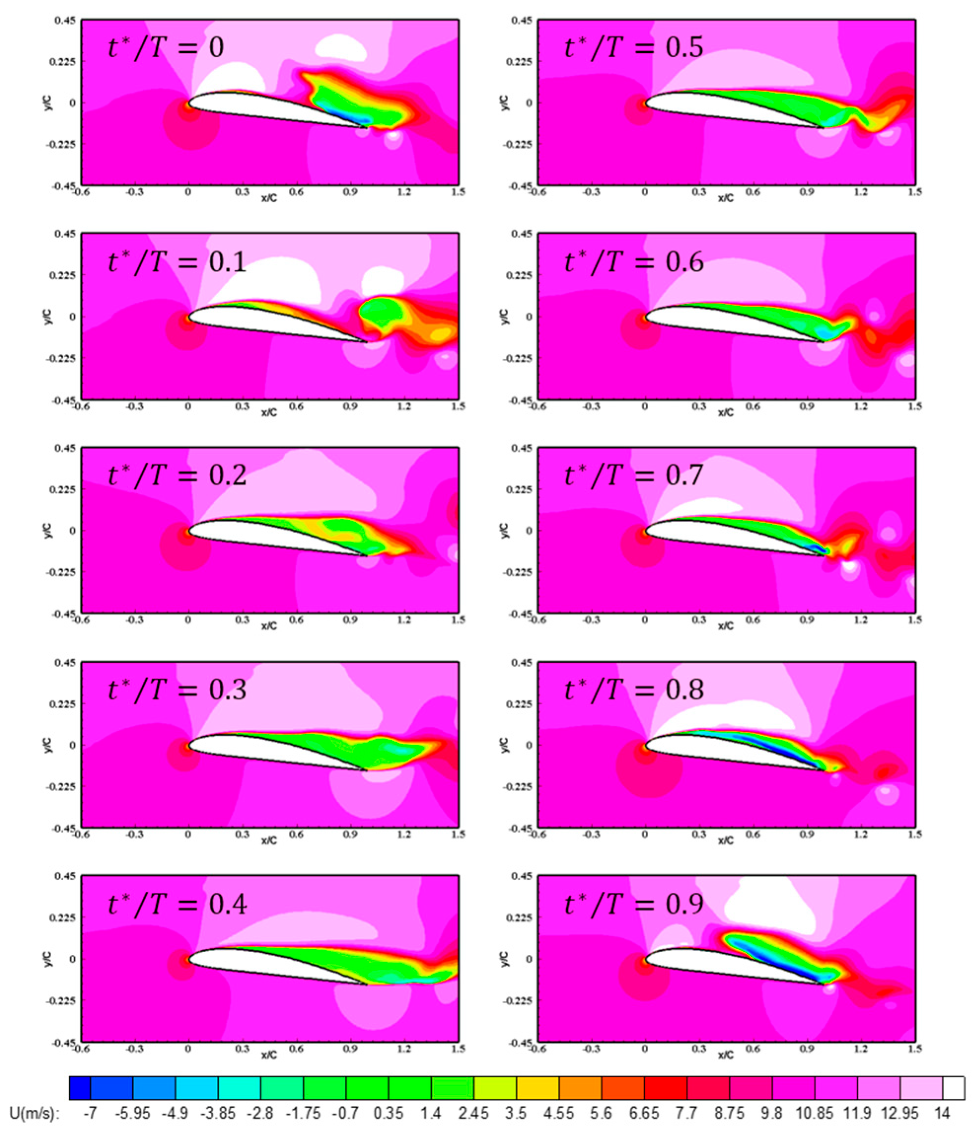
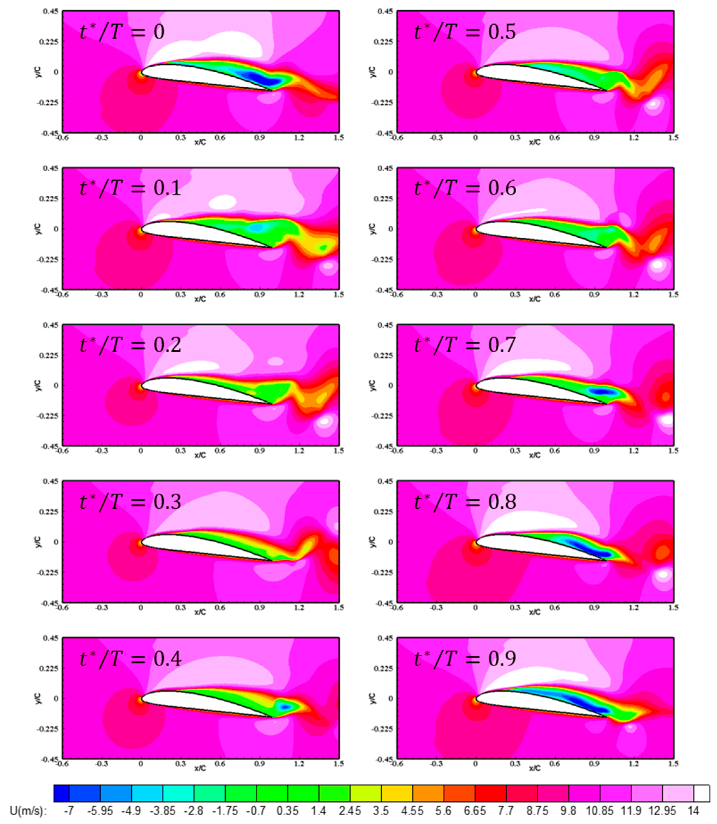
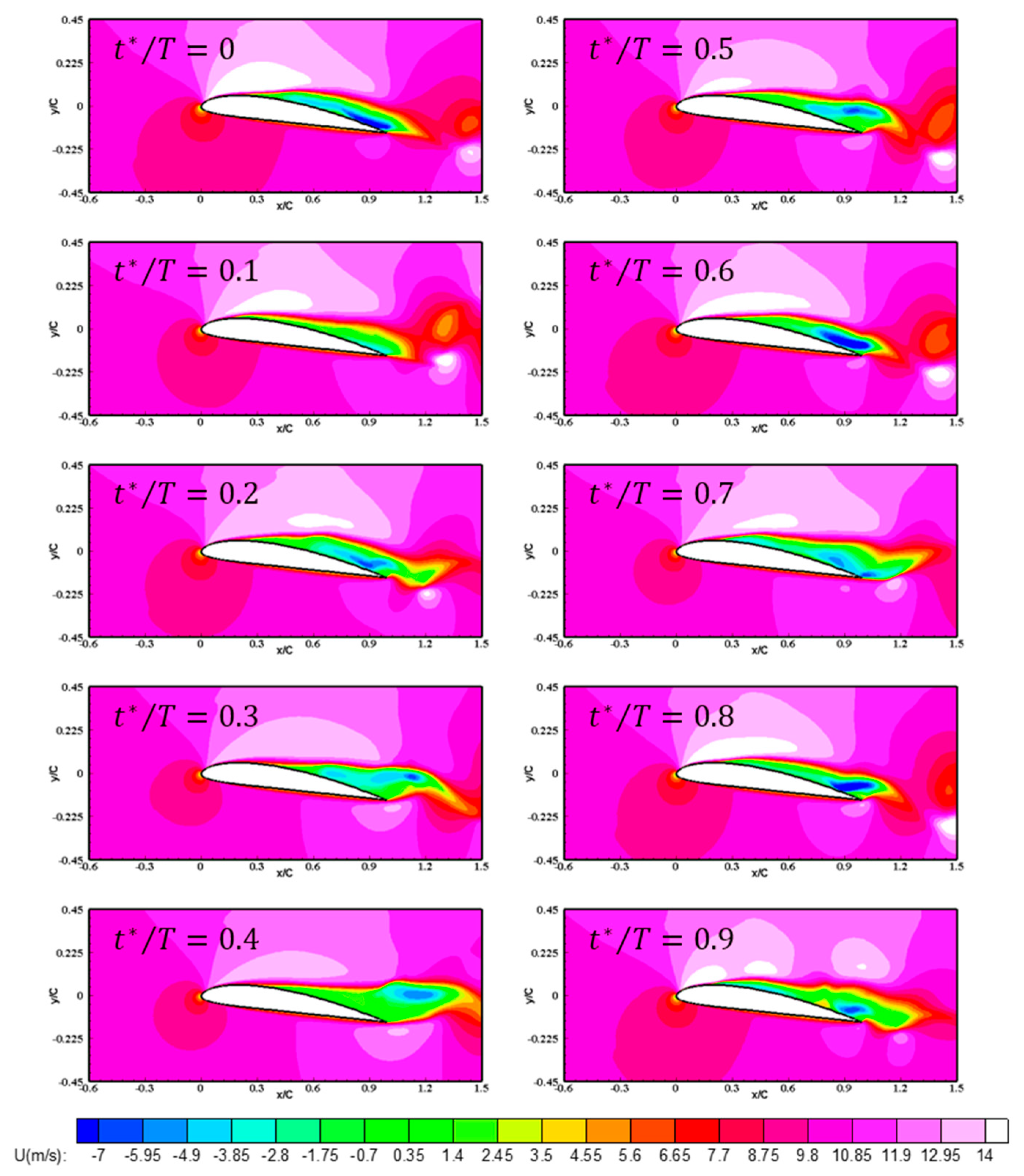
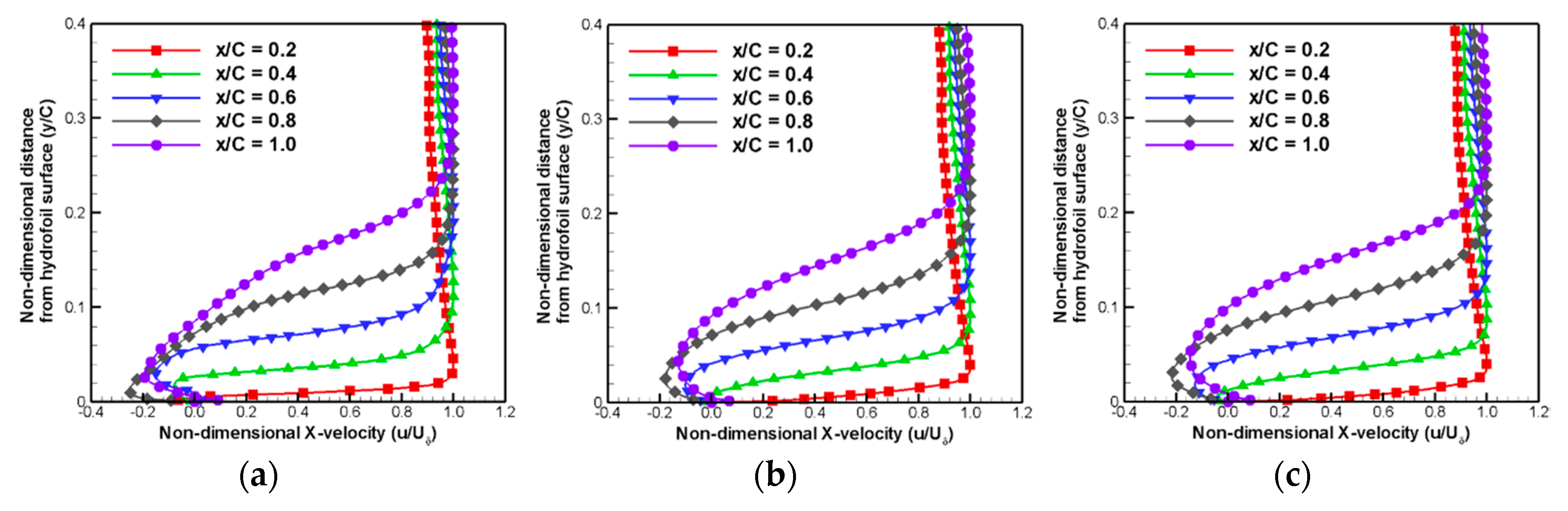
The reason why these predicted results among three different viscous flux treatment methods show quite different cavity structures can be identified from the velocity field around the hydrofoil. Figure 12, Figure 13 and Figure 14 compare the iso-contours of the predicted distributions of the stream-wise (x-direction) velocities, of the three different viscous models, during a single cycle. As reported in several previous studies [3,42,43,44], the re-entrant jet is the most critical mechanism causing unstable cavitation behavior. The re-entrant jet causes adverse velocity gradients on hydrofoil surfaces in a stream-wise direction, and then back-flow toward the leading edge occurs. This back-flow eventually breaks the cavity structures such that the most developed cavity structure is split into two, and the trailing edge cavities are shed downstream. As shown in the Figure 12, Figure 13 and Figure 14, re-entrant jet phenomena can be seen in the suction side of hydrofoil. In order to compare the strength of re-entrant jet for three viscous cases, the time-averaged x-directional velocity profile is examined. Figure 15 shows the distribution of time-averaged x-direction velocities at different locations for the three viscous cases. As can be seen in Figure 15, all three cases exhibit similar velocity profiles, and velocity values, at the outer cavity region. However, in the inner cavity region, the profiles differ significantly.
Figure 16 shows zoomed-in plots of the x-direction velocity profiles at x/C = 0.4 and x/C = 0.6. The viscous lagging approach exhibits a stronger re-entrant jet phenomenon than the thin-layer and full viscous cases. The over-predicted re-entrant jet results in larger shed cavity structures than the other two cases. Consequently, the viscous lagging approach exhibits significantly different results from the experimental result, in terms of the cavity distribution.
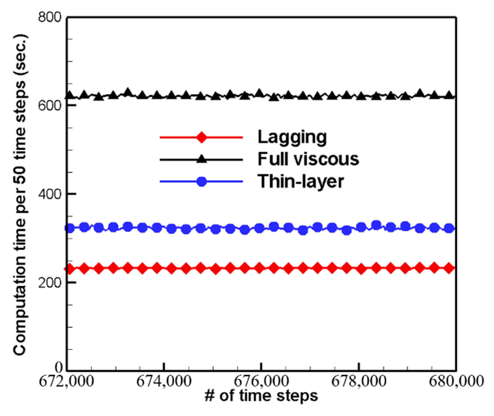
In Figure 17, the required computation times per 50 time steps are compared for the three different viscous cases. As can be seen, the viscous lagging approach requires less computation time than the other approaches, and the thin-layer approach requires approximately half that of the full viscous approach. Based on the above results, it can be concluded that the thin-layer approach can be used as an alternative for the full viscous approach in terms of accuracy and efficiency.
4.3. Viscous Effects on Hydro-Acoustic Field Prediction
Hydro-acoustic fields due to the cavitation flow of the Clark-Y hydrofoil are predicted using the integral from of the FW-H equation, with an input from the results of the predicted flow fields discussed in the previous section. The predicted hydro-acoustic fields are compared in terms of noise directivity and spectrum between the three viscous models used for the flow simulation.
The time variation of cavity volume changes is used to model the monopole source term that is the first term in the right-hand side of Equation (19). The volume integration is conducted over the volume containing all the developed cavity structure. For the dipole source that is the second term in the right-hand side of Equation (19), hydrodynamic forces on the hydrofoil surfaces are used directly in terms of lift and drag forces. Therefore, the surface integration is conducted over the hydrofoil surfaces. The variation in the retarded time is neglected because the Helmholtz number based on the chord length of the hydrofoil is around 0.47 at 10 kHz. For the extraction of source data, the flow field results are saved every 50-time steps (2.6 × 10⁻⁵ s.) and total three-cycle data are used. The predicted acoustic wave directivity for each case is presented in Figure 15.
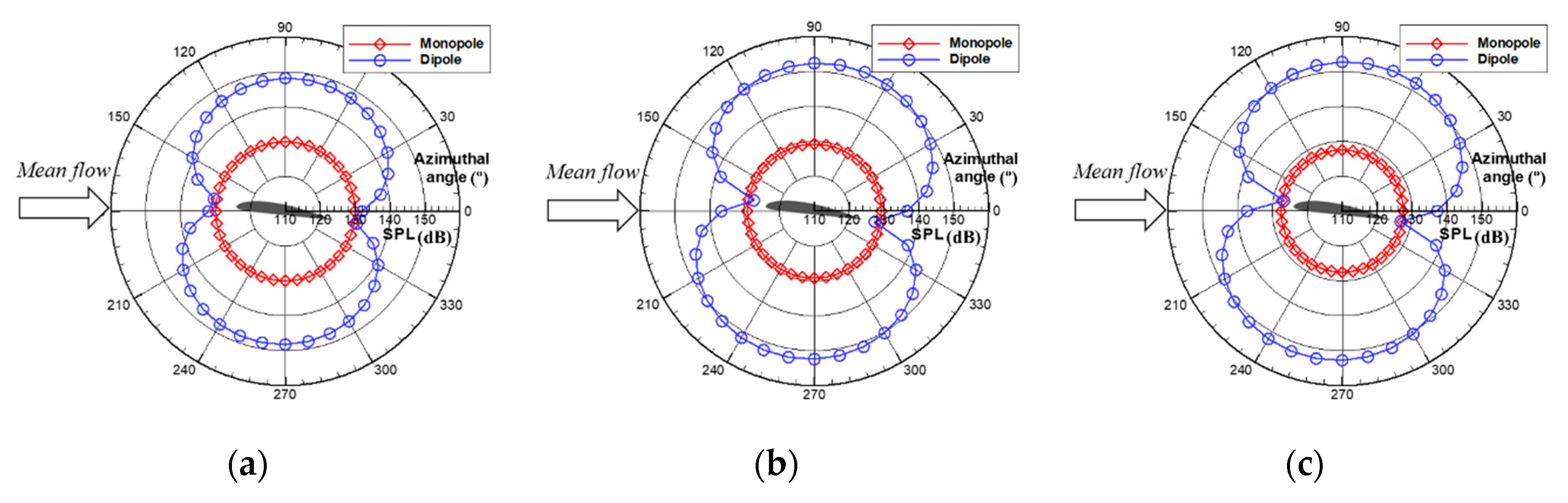
As can be seen in Figure 18, the three cases exhibit similar propagation patterns where the lift dipole is dominant. In the case of the dipole source term, the radiating pattern has two lobes with a 180° phase difference. The main direction of the lobes depends on the dominance of the lift or drag dipole forces. As shown in Figure 3, the lift time-variation is significantly greater than that of drag, therefore, hydro-acoustic waves due to dipole sources are affected primarily by the lift force, and thus exhibit the lift-dipolar pattern. Here, the directivity is inclined with respect to the mean flow due to the angle of attack. However, the directivity due to the monopole source exhibits an omni-directional radiation pattern, as it depends on the time derivative.
The predicted sound pressure levels (SPL) of each noise source for the three viscous cases are compared in Figure 19 and Figure 20. For the monopole source component, the viscous lagging approach has the largest SPLs, whereas the thin-layer approach presents the smallest SPLs. These results can be explained qualitatively by comparing the observed cavity sizes. With the viscous lagging approach, the largest cavity structures are predicted. This leads to the largest SPLs of the monopole sources, as shown in Figure 5, Figure 6, Figure 7, Figure 8 and Figure 9, as the monopole source strength is typically proportional to the time variation of cavity volume changes. Note that, because a monopole has an omni-directional radiation pattern, the predicted acoustic pressure spectrum due to monopole sources at different azimuth angles has the same values.
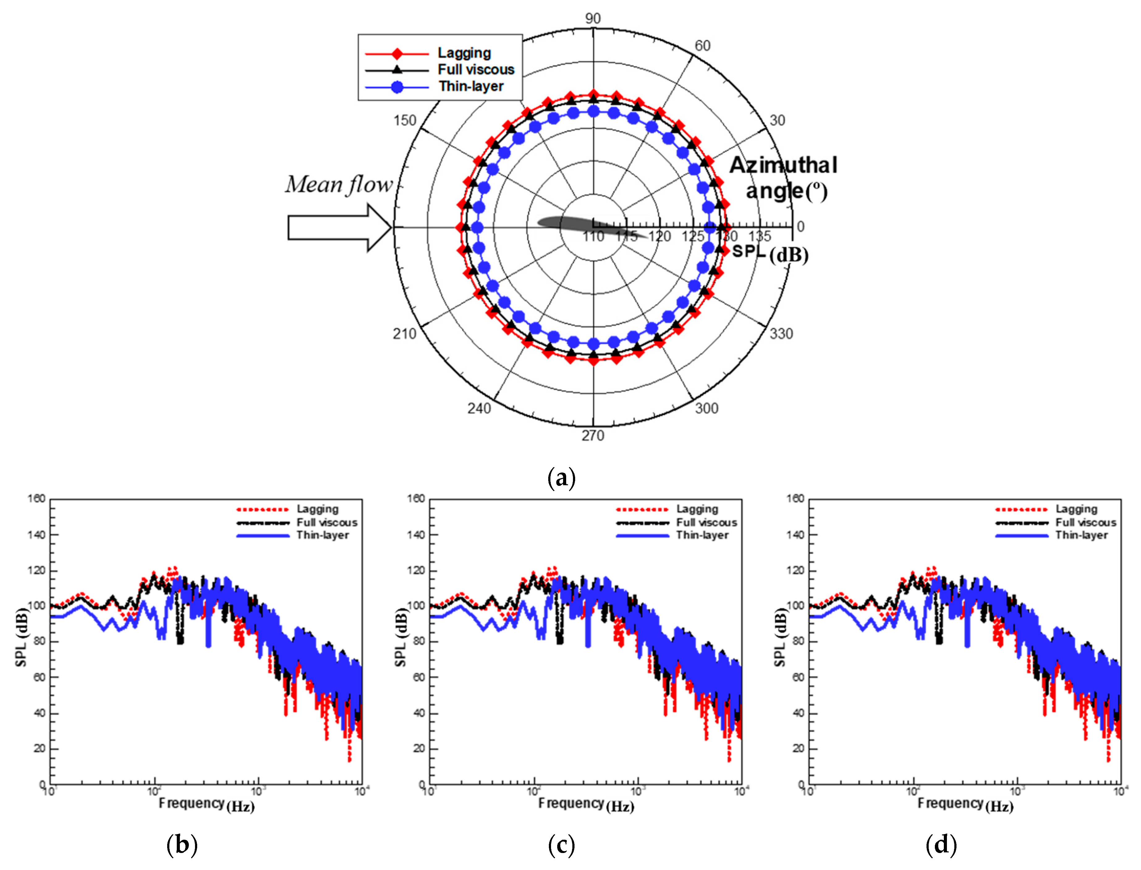
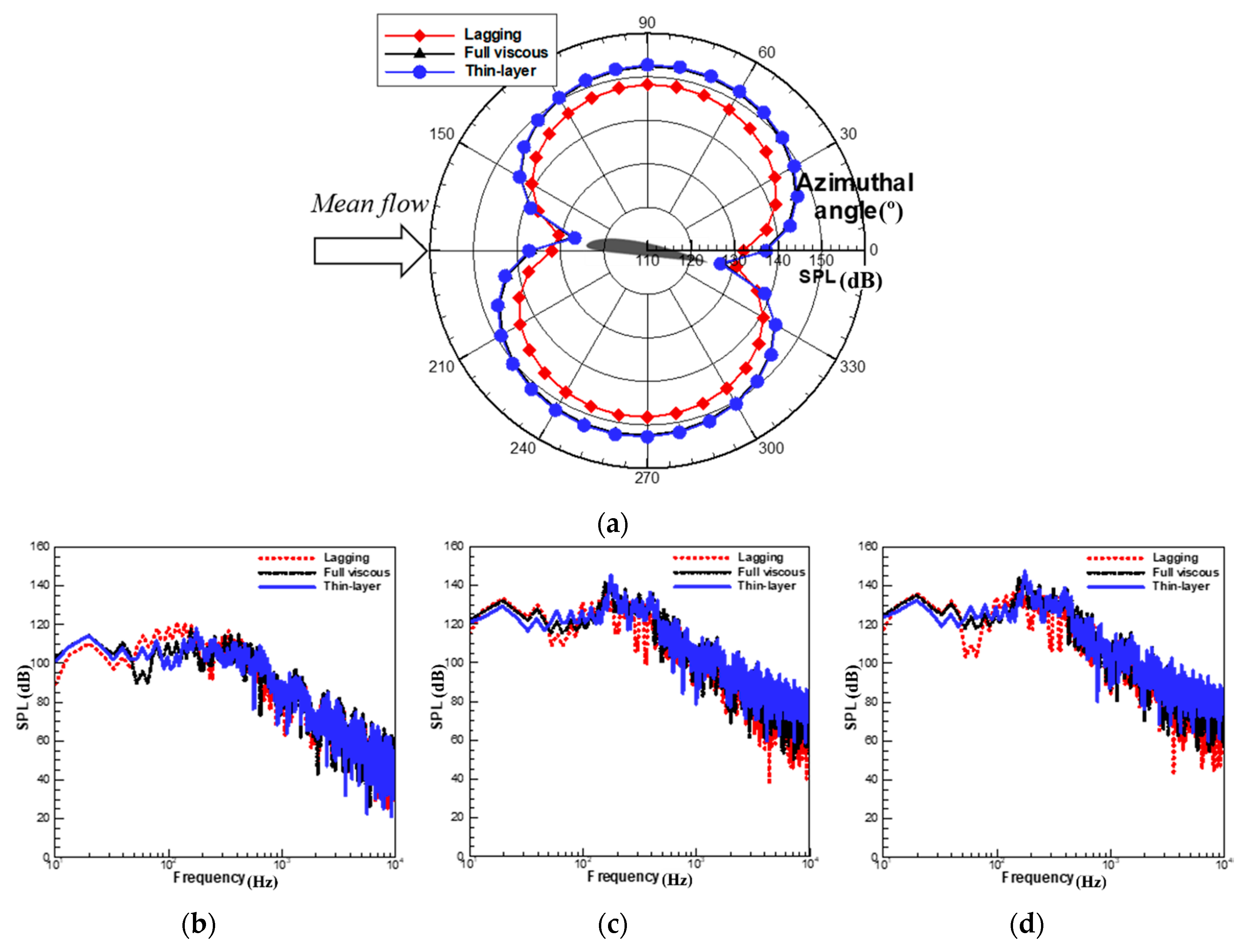
In the case of dipolar noise source components, the thin-layer and full viscous cases exhibit approximately the same SPLs, but the viscous lagging approach has the lowest SPLs, except at azimuth angles of 350° and 170°. These results are related to the variation of hydro-dynamic forces. As shown in Figure 4, the viscous lagging approach exhibits lower spectral magnitudes across the entire frequency range for the lift force, and f ≥200 Hz for the drag force. Therefore, compared to the thin layer and full viscous methods, smaller SPLs are observed at the locations where the lift forces are dominant, whereas larger SPLs are predicted at the locations where the drag forces are dominant (azimuth angles of 350° and 170°). However, the overall SPL directivity, and the predicted spectrum, of the thin layer approach closely follow those of the full viscous method.
Table 3 compares the predicted acoustic power levels (PWLs) of the cavitating hydrofoil. It is again seen that the thin-layer model presents almost the same acoustic power levels as the full viscous model.
5. Conclusions
In this study, the effects of viscous flux vectors on cavitation flow, and its radiated flow noise, of the Clark Y hydrofoil were numerically examined using computational fluid dynamics techniques and the Ffowcs Williams–Hawkings acoustic analogy. For the flow field analysis, the full 3D unsteady compressible RANS equations, coupled with the homogeneous mixture model, was applied. The hydro-acoustic field was predicted by solving the FW-H equation based on the information of monopole and dipole sources from the predicted flow field results, under the assumption of compact sources. The time-variation of cavity volume changes, and the hydro-dynamic forces on the hydrofoil surfaces, were used to determine the monopole and dipole source strength. The effects of viscous flux were examined by modeling the viscous flux terms in three different approximation approaches: the viscous lagging, the thin-layer, and the full viscous approaches. All three models exhibited similar periodic behaviors of generation, development, and extinction of cavitation, at the same 20 Hz fundamental frequency. However, the detailed unsteady behaviors differed significantly, especially between the viscous lagging method and the other two methods. The viscous lagging approach exhibited a tendency to over-predict the cavity structure and re-entrant jet, and to predict lower fluctuating hydro-dynamic forces. This resulted in larger SPLs for the monopolar noise components, but smaller SPLs for the dipolar noise components, than the other two cases. However, the thin-layer approach results were the closest to those of the full viscous model, in terms of the time-variation of hydro-dynamic loading and liquid volume fraction as characteristics of the predicted flow field, and the directivities and spectrum of the radiated acoustic field. However, it marginally under-predicted the leading-edge cavitation, and over-predicted the dissipation of shed cavities, and thus exhibited smaller SPLs because of monopolar noise. Based on these results, the thin layer approach can be proposed as an effective and efficient method for investigating the two-phase flow noise of hydrofoils as an alternative to the full viscous approach.
Acknowledgments
This work was supported by the Ministry of Trade, Industry and Energy, MOTIE (project code: 10045337).
Author Contributions
Warn-Gyu Park developed the original CFD code. Cheolung Cheong proposed the original idea motivating the present research. Sanghyeon Kim upgraded the original code by adding the filter-based turbulence models and additional viscous flux treatments (full viscous and thin-layer models), carried out the numerical simulations and prepared all of data. The relevant numerical analysis was carried out by both of Sanhyeon Kim and Cheolung Cheong.
Conflicts of Interest
The authors declare no conflict of interest.
References
- Shen, Y.T.; Dimotakis, P.E. The influence of surface cavitation on hydrodynamic forces. In Proceedings of the 22nd American Towing Tank Conference, St. John’s, NL, Canada, 8–11 August 1989. [Google Scholar]
- Kawanami, H.; Kato, H.; Yamaguchi, H.; Tanimura, M.; Tagaya, Y. Mechanism and control of cloud cavitation. J. Fluids Eng. 1997, 119, 788–794. [Google Scholar] [CrossRef]
- Wang, G.; Senocak, I.; Shyy, W.; Ikohagi, T.; Cao, S. Dynamics of attached turbulent cavitating flows. Prog. Aerosp. Sci. 2001, 37, 551–581. [Google Scholar] [CrossRef]
- Park, C.; Seol, H.; Kim, K.; Seong, W. A study on propeller noise source localization in a cavitation tunnel. Ocean Eng. 2009, 36, 754–762. [Google Scholar] [CrossRef]
- Kopriva, J.; Arndt, R.E.A.; Amromin, E.L. Improvement of hydrofoil performance by partial ventilated cavitation in steady flow and periodic gusts. J. Fluids Eng. 2008, 130, 031301. [Google Scholar] [CrossRef]
- Karn, A.; Arndt, R.E.A.; Hong, J. Dependence of supercavity closure upon flow unsteadiness. Exp. Therm. Fluid Sci. 2015, 68, 493–498. [Google Scholar] [CrossRef]
- Merkle, C.L.; Feng, J.H.; Buelow, P.E.O. Computational modeling of the dynamics of sheet cavitation. In Proceedings of the 3rd International Symposium on Cavitation, Grenoble, France, 7–10 April 1998. [Google Scholar]
- Singhal, A.K.; Athavale, M.M.; Li, H.; Jiang, Y. Mathematical basis and validation of the full cavitation model. J. Fluids Eng. 2002, 124, 617–624. [Google Scholar] [CrossRef]
- Kunz, R.F.; Boger, D.A.; Stinebrin, D.R.; Chyczewsky, T.S.; Lindau, J.W.; Gilbeling, H.J.; Venkateswaran, S.; Govindan, T.R. A preconditioned Navier-Stokes method for two-phase flows with application to cavitation prediction. Comput. Fluids 2000, 29, 849–875. [Google Scholar] [CrossRef]
- Huang, D.G. Preconditioned dual-time procedures and its application to simulating the flow with cavitations. J. Comput. Phys. 2007, 223, 685–689. [Google Scholar] [CrossRef]
- Esfahanian, V.; Akbarzadeh, P. Numerical investigation on a new local preconditioning method for solving the incompressible inviscid, non-cavitating and cavitating flows. J. Frankl. Inst. 2011, 348, 1208–1230. [Google Scholar] [CrossRef]
- Ha, C.T.; Park, W.G. Evaluation of a new scaling term in preconditioning schemes for computations of compressible cavitating and ventilated flows. Ocean Eng. 2016, 126, 432–466. [Google Scholar] [CrossRef]
- Johansen, S.T.; Wu, J.; Shyy, W. Filter-based unsteady RANS computations. Int. J. Heat Fluid Flow 2004, 25, 10–21. [Google Scholar] [CrossRef]
- Tseng, C.; Wang, L. Investigation of empirical coefficients of cavitation and turbulence model through steady and unsteady turbulent cavitating flows. Comput. Fluids 2014, 103, 262–274. [Google Scholar] [CrossRef]
- Zhang, D.; Wang, H.; Shi, W.; Zhang, G.; Van Esch, B.B. Numerical analysis of the unsteady behavior of cloud cavitation around a hydrofoil based on an improved filter-based model. J. Hydrodyn. 2015, 27, 795–808. [Google Scholar] [CrossRef]
- Kim, S.; Cheong, C.; Park, W.G. Numerical investigation on cavitation flow of hydrofoil and its flow noise with emphasis on turbulence models. AIP Adv. 2017, 7, 065114. [Google Scholar] [CrossRef]
- Venkateswaran, S.; Merkle, C.L. Dual time stepping and preconditioning for unsteady computations. In Proceedings of the 33rd Aerospace Sciences Meeting and Exhibit, Reno, NV, USA, 9–12 January 1995. [Google Scholar]
- Venkateswaran, S.; Lindau, J.W.; Kunz, R.F.; Merkle, C.L. Preconditioning algorithms for the computation of multi-phase mixture flows. In Proceedings of the 39th Aerospace Sciences Meeting and Exhibit, Reno, NV, USA, 8–11 January 2001. [Google Scholar]
- Owis, F.M.; Nayfeh, A.H. Numerical simulation of 3-D incompressible, multi-phase flows over cavitating projectiles. Eur. J. Mech. B Fluids 2004, 23, 339–351. [Google Scholar] [CrossRef]
- Wagner, W.; Kretzschmar, H. International Steam Tables: Properties of Water and Steam Based on the Industrial Formulation IAPWS0IF97, 2nd ed.; Springer Science & Business Media: Berlin/Heidelberg, Germany, 2007; ISBN 978-3-540-21419-9. [Google Scholar]
- Jones, W.P.; Launder, B.E. The prediction of laminarization with a two-equation model of turbulence. Int. J. Heat Mass Transf. 1972, 15, 301–314. [Google Scholar] [CrossRef]
- Jones, W.P.; Launder, B.E. The calculation of low-Reynolds-number phenomena with a two-equation model of turbulence. Int. J. Heat Mass Transf. 1973, 16, 1119–1130. [Google Scholar] [CrossRef]
- Hoffmann, K.A. Chiang, S.T. Computational Fluid Dynamics, 4th ed.; Engineering Education System: Wichita, KS, USA, 2000; ISBN 978-0962373107. [Google Scholar]
- Beam, R.M.; Warming, R.F. An implicit factored scheme for the compressible Navier-Stokes equations. AIAA J. 1978, 16, 393–402. [Google Scholar] [CrossRef]
- Steger, J.L. Implicit finite-difference simulation of flow about arbitrary two-dimensional geometries. AIAA J. 1978, 16, 679–686. [Google Scholar] [CrossRef]
- Pletcher, R.; Chen, K. On solving the compressible Navier-Stokes equations for unsteady flows at very low Mach number. In Proceedings of the 11th Computational Fluid Dynamics Conference, Orlando, FL, USA, 6–9 July 1993. [Google Scholar]
- Wang, Y.; Sun, X.J.; Zhu, B.; Zhang, H.J.; Huang, D.G. Effect of blade vortex interaction on performance of Darrieus-type cross flow marine current turbine. Renew. Energy 2016, 86, 316–323. [Google Scholar] [CrossRef]
- Granier, B.; Lerat, A.; Wu, Z. An implicit centered scheme for steady and unsteady incompressible one and two-phase flows. Comput. Fluids 1997, 26, 373–393. [Google Scholar] [CrossRef]
- Senocak, I.; Shyy, W. A pressure-based method for turbulent cavitating flow computations. J. Comput. Phys. 2001, 176, 363–383. [Google Scholar] [CrossRef]
- Pulliam, T.H.; Steger, J.L. Implicit finite-difference simulations of three-dimensional compressible flow. AIAA J. 1980, 18, 159–167. [Google Scholar] [CrossRef]
- Tysinger, T.L.; Caughey, D.A. Implicit multigrid algorithm for the Navier-Stokes equations. In Proceedings of the 29th Aerospace Sciences Meeting, Reno, NV, USA, 7–10 January 1991. [Google Scholar]
- Ffowcs Williams, J.E.; Hawkings, D.L. Sound generation by turbulence and surfaces in arbitrary motion. Philos. Trans. R. Soc. A 1969, 264, 321–342. [Google Scholar] [CrossRef]
- Singer, B.A.; Lockard, D.P.; Lilley, G.M. Hybrid acoustic preditions. Comput. Math. Appl. 2003, 46, 647–669. [Google Scholar] [CrossRef]
- Khorrami, M.R.; Singer, B.A.; Berkman, M.E. Time-accurate simulations and acoustic analysis of slat free shear layer. AIAA J. 2002, 40, 1284–1291. [Google Scholar] [CrossRef]
- Wang, M.; Freund, J.B.; Lele, S.K. Computational prediction of flow-generated sound. Annu. Rev. Fluid Mech. 2006, 38, 483–512. [Google Scholar] [CrossRef]
- Farassat, F.; Casper, J.H. Toward an airframe noise prediction methodology: Survey of current approaches. In Proceedings of the 44th Aerospace Sciences Meeting and Exhibit, Reno, NV, USA, 9–12 January 2006. [Google Scholar]
- Lighthill, M.J. On sound generated aerodynamically. I. General theory. Proc. R. Soc. Lond. A Math. Phys. Sci. 1952, 211, 564–587. [Google Scholar] [CrossRef]
- Lighthill, M.J. On sound generated aerodynamically. II. Turbulence as a source of sound. Proc. R. Soc. Lond. A Math. Phys. Sci. 1954, 222, 1–32. [Google Scholar] [CrossRef]
- Curle, N. The influence of solid boundaries upon aerodynamic sound. Proc. R. Soc. Lond. A Math. Phys. Eng. Sci. 1955, 231, 505–514. [Google Scholar] [CrossRef]
- Roohi, E.; Zahiri, A.P.; Passandideh-Fard, M. Numerical simulation of cavitation around a two-dimensional hydrofoil using VOF method and LES turbulence model. Appl. Math. Model. 2013, 37, 6469–6488. [Google Scholar] [CrossRef]
- Huang, B.; Young, Y.L.; Wang, G.; Shyy, W. Combined experimental and computational investigation of unsteady structure of sheet/cloud cavitation. J. Fluids Eng. 2013, 135, 071301. [Google Scholar] [CrossRef]
- Watanabe, S.; Tsujimoto, Y.; Furukawa, A. Theoretical analysis of transitional and partial cavity instabilities. J. Fluids Eng. 2001, 123, 692–697. [Google Scholar] [CrossRef]
- Leroux, J.B.; Coutier-Delgosha, O.; Astolfi, J.A. A joint experimental and numerical study of mechanisms associated to instability of partial cavitation on two-dimensional hydrofoil. Phys. Fluids 2005, 17, 052101. [Google Scholar] [CrossRef]
- Coutier-Delgosha, O.; Stutz, B.; Vabre, A.; Legoupil, S. Analysis of cavitating flow structure by experimental and numerical investigations. J. Fluid Mech. 2007, 578, 171–222. [Google Scholar] [CrossRef]
Figure 1.
(a) Computational domain and (b) zoomed grid system.

Figure 2.
Comparison of predicted pressure coefficient distribution with large eddy simulation (LES) data by Roohi et al. [40].
Figure 2.
Comparison of predicted pressure coefficient distribution with large eddy simulation (LES) data by Roohi et al. [40].

Figure 3.
Comparison of time-averaged x-directional velocity distribution with experimental results by Huang et al. [41]: (a) ; (b) ; (c) ; (d) ; and (e) .
Figure 3.
Comparison of time-averaged x-directional velocity distribution with experimental results by Huang et al. [41]: (a) ; (b) ; (c) ; (d) ; and (e) .


Figure 4.
Predicted time-variation and power spectral density of non-dimensional hydrodynamic forces: (a) lift force; (b) drag force.
Figure 4.
Predicted time-variation and power spectral density of non-dimensional hydrodynamic forces: (a) lift force; (b) drag force.


Figure 5.
Time-variations of predicted cavity volume of three different viscous flux vector treatment methods.
Figure 5.
Time-variations of predicted cavity volume of three different viscous flux vector treatment methods.

Figure 6.
Time-variation of predicted liquid volume fraction in viscous lagging case.

Figure 7.
Time-variation of predicted liquid volume fraction in full viscous case.

Figure 8.
Time-variation of predicted liquid volume fraction in thin-layer case.

Figure 9.
Comparison of instantaneous cavitation structures in the trailing edge region.

Figure 10.
Time-averaged vapor volume fraction distribution at five stream-wise locations: (a) viscous lagging; (b) full viscous; and (c) thin-layer cases.
Figure 10.
Time-averaged vapor volume fraction distribution at five stream-wise locations: (a) viscous lagging; (b) full viscous; and (c) thin-layer cases.

Figure 11.
Comparison of zoomed time-averaged vapor volume fraction distribution for three different viscous flux treatment methods at five stream-wise locations: (a) ; (b) ; (c) ; (d) ; and (e) .
Figure 11.
Comparison of zoomed time-averaged vapor volume fraction distribution for three different viscous flux treatment methods at five stream-wise locations: (a) ; (b) ; (c) ; (d) ; and (e) .


Figure 12.
Time-variation of predicted x-directional velocity: viscous lagging case.

Figure 13.
Time-variation of predicted x-directional velocity: full viscous case.

Figure 14.
Time-variation of predicted x-directional velocity: thin-layer case.

Figure 15.
Time-averaged x-directional velocity distribution at five stream-wise locations: (a) viscous lagging; (b) full viscous; and (c) thin-layer cases.
Figure 15.
Time-averaged x-directional velocity distribution at five stream-wise locations: (a) viscous lagging; (b) full viscous; and (c) thin-layer cases.

Figure 16.
Comparison of zoomed time-averaged x-directional velocity distribution with experimental results by Huang et al. [40]: (a) x/C = 0.4; and (b) x/C = 0.6.
Figure 16.
Comparison of zoomed time-averaged x-directional velocity distribution with experimental results by Huang et al. [40]: (a) x/C = 0.4; and (b) x/C = 0.6.

Figure 17.
Comparison of required computational time per 50 time steps for three viscous cases.

Figure 18.
Predicted directivity of radiated hydro-acoustic noise: (a) viscous lagging; (b) fill viscous; and (c) thin-layer cases.
Figure 18.
Predicted directivity of radiated hydro-acoustic noise: (a) viscous lagging; (b) fill viscous; and (c) thin-layer cases.

Figure 19.
Predicted hydro-acoustic pressure due to monopole source: (a) directivity, spectrum at three azimuth angles of (b) 350°; (c) 40°; and (d) 80°.
Figure 19.
Predicted hydro-acoustic pressure due to monopole source: (a) directivity, spectrum at three azimuth angles of (b) 350°; (c) 40°; and (d) 80°.

Figure 20.
Predicted hydro-acoustic pressure due to dipole source: (a) directivity, spectrum at three azimuth angles of (b) 350°; (c) 40°; and (d) 80°.
Figure 20.
Predicted hydro-acoustic pressure due to dipole source: (a) directivity, spectrum at three azimuth angles of (b) 350°; (c) 40°; and (d) 80°.


Table 1.
Computational conditions.
| Parameters | (m/s) | (m) | Angle of Attack (°) | ||
|---|---|---|---|---|---|
| Values | 0.8 | 10 | 0.07 | 8 |
Table 2.
Comparison of time-averaged non-dimensional cavity thickness with experimental results by Wang et al. [3].
Table 2.
Comparison of time-averaged non-dimensional cavity thickness with experimental results by Wang et al. [3].
| Location | Experiments | Viscous Lagging | Full Viscous | Thin-Layer |
|---|---|---|---|---|
| 0.0195 | 0.0285 | 0.0280 | 0.0286 | |
| 0.0658 | 0.0811 | 0.0738 | 0.0748 | |
| 0.1166 | 0.1529 | 0.1245 | 0.1234 | |
| 0.1834 | 0.2161 | 0.1798 | 0.1737 | |
| 0.2339 | 0.2637 | 0.2324 | 0.2198 |
Table 3.
Estimated acoustic power levels (dB) for three different viscous flux models according to source types. PWL: predicted acoustic power level.
Table 3.
Estimated acoustic power levels (dB) for three different viscous flux models according to source types. PWL: predicted acoustic power level.
| Viscous Flux Treatment | Viscous Lagging | Full Viscous | Thin-Layer |
|---|---|---|---|
| PWL (dB) | 168.8 | 177.1 | 177.4 |
© 2018 by the authors. Licensee MDPI, Basel, Switzerland. This article is an open access article distributed under the terms and conditions of the Creative Commons Attribution (CC BY) license (http://creativecommons.org/licenses/by/4.0/).
Share and Cite
MDPI and ACS Style
Kim, S.; Cheong, C.; Park, W.-G. Numerical Investigation into Effects of Viscous Flux Vectors on Hydrofoil Cavitation Flow and Its Radiated Flow Noise. Appl. Sci. 2018, 8, 289. https://0-doi-org.brum.beds.ac.uk/10.3390/app8020289
AMA Style
Kim S, Cheong C, Park W-G. Numerical Investigation into Effects of Viscous Flux Vectors on Hydrofoil Cavitation Flow and Its Radiated Flow Noise. Applied Sciences. 2018; 8(2):289. https://0-doi-org.brum.beds.ac.uk/10.3390/app8020289
Chicago/Turabian StyleKim, Sanghyeon, Cheolung Cheong, and Warn-Gyu Park. 2018. "Numerical Investigation into Effects of Viscous Flux Vectors on Hydrofoil Cavitation Flow and Its Radiated Flow Noise" Applied Sciences 8, no. 2: 289. https://0-doi-org.brum.beds.ac.uk/10.3390/app8020289
Note that from the first issue of 2016, this journal uses article numbers instead of page numbers. See further details here.