Bias Impact Analysis and Calibration of UAV-Based Mobile LiDAR System with Spinning Multi-Beam Laser Scanner

Abstract

Light Detection and Ranging (LiDAR) is a technology that uses laser beams to measure ranges and generates precise 3D information about the scanned area. It is rapidly gaining popularity due to its contribution to a variety of applications such as Digital Building Model (DBM) generation, telecommunications, infrastructure monitoring, transportation corridor asset management and crash/accident scene reconstruction. To derive point clouds with high positional accuracy, estimation of mounting parameters relating the laser scanners to the onboard Global Navigation Satellite System/Inertial Navigation System (GNSS/INS) unit, i.e., the lever-arm and boresight angles, is the foremost and necessary step. This paper proposes a LiDAR system calibration strategy for a Unmanned Aerial Vehicle (UAV)-based mobile mapping system that can directly estimate the mounting parameters for spinning multi-beam laser scanners through an outdoor calibration procedure. This approach is based on the use of conjugate planar/linear features in overlapping point clouds derived from different flight lines. Designing an optimal configuration for calibration is the first and foremost step in order to ensure the most accurate estimates of mounting parameters. This is achieved by conducting a rigorous theoretical analysis of the potential impact of bias in mounting parameters of a LiDAR unit on the resultant point cloud. The dependency of the impact on the orientation of target primitives and relative flight line configuration would help in deducing the configuration that would maximize as well as decouple the impact of bias in each mounting parameter so as to ensure their accurate estimation. Finally, the proposed analysis and calibration strategy are validated by calibrating a UAV-based LiDAR system using two different datasets—one acquired with flight lines at a single flying height and the other with flight lines at two different flying heights. The calibration performance is evaluated by analyzing correlation between the estimated system parameters, the a-posteriori variance factor of the Least Squares Adjustment (LSA) procedure and the quality of fit of the adjusted point cloud to planar/linear features before and after the calibration process.

1. Introduction

LiDAR-based data acquisition is gaining widespread recognition as an efficient and cost-effective technique for rapid collection of 3D geospatial data. The main factors behind the widespread use of LiDAR systems include the continuous improvement in GNSS/INS direct geo-referencing technology as well as enhanced performance and reduced size and cost of laser scanning units. Currently, there are commercially available LiDAR units that are capable of emitting more than a quarter million pulses per second at a cost of less than $10 k. Such availability, together with the increasing range of applications—such as digital building model generation, transportation corridor monitoring, telecommunications, precision agriculture, infrastructure monitoring, seamless outdoor-indoor mapping, power line clearance evaluation and crash scene reconstruction [1,2,3,4,5]—have led to the development of multi-unit mobile LiDAR systems onboard airborne and terrestrial platforms that are either manned or unmanned. However, the attainment of the full positioning potential of such systems is contingent on an accurate calibration of the mobile mapping unit as a whole, wherein we need to estimate the mounting parameters relating the onboard units and the internal characteristics of the sensor.

Some of the applications mentioned above can be effectively met using UAV platforms [5,6,7,8]. The sensors onboard a UAV platform need to be commensurate with the payload restrictions as well as their effectiveness for the desired mapping and monitoring application. The cost-effective Velodyne laser scanner (a spinning multi-beam laser unit) can rapidly capture a high volume of data and has been used in many mobile mapping systems and robotics applications [9,10,11]. Over the past few years, a great deal of research has been devoted to modeling the inherent systematic errors in Velodyne laser scanners as well as the calibration of LiDAR systems to estimate the internal sensor characteristics and mounting parameters [12,13]. Glennie et al. (2016) [14] performed a geometric calibration with stationary VLP-16 to marginally improve the accuracy of the point clouds by approximately 20%. Moreover, they also investigated the range accuracy of VLP-16, which is quoted to have a Root Mean Square Error (RMSE) value between 22 and 27 mm in the factory supplied calibration certificate. But, it was observed that some of the laser beams have worse range accuracy than others. Although many LiDAR system calibration procedures have been developed in the past, outdoor calibration of integrated GNSS/INS and multi-unit 3D laser scanners is still an active area of research.

The major contribution of this work is to develop an optimal/minimal flight and feature configuration for a reliable estimation of mounting parameters. In this regard, minimal refers to the minimal number of flight lines and feature configuration that are required for reliable calibration. On the other hand, optimal denotes decoupling (removing any significant correlation between) various components of the mounting parameters. This can be achieved through a bias impact analysis that evaluates the effect of biases in the mounting on features with different configurations. Before proceeding with the bias impact analysis, we first introduce the components involved in the UAV-based LiDAR system used in this research and discuss the details regarding the synchronization of the hardware units (LiDAR and GNSS/INS units). Then, we focus on developing a calibration strategy for a UAV-based LiDAR system with a spinning multi-beam laser scanner by conducting an in-depth analysis of the impact of biases in the system parameters on the resultant 3D point cloud. The purpose of system calibration is to simultaneously estimate the mounting parameters relating the different system components by minimizing the discrepancy between conjugate linear and/or planar features in overlapping point clouds derived from different flight lines. In this regard, a detailed bias impact analysis facilitates the design of an optimal configuration of target primitives and flight lines for ensuring accurate calibration results. Habib et al. (2010) [15] discussed the bias impact analysis in detail for airborne linear scanners while describing the simplified and quasi-rigorous approaches for calibration, whereas in this research, the bias impact analysis is conducted for a spinning multi-beam laser scanner starting from the 3D point-positioning equation. The optimal target primitive configuration is devised by studying the impact of biases on planes oriented in different directions and the optimal flight line configuration is determined based on the effect of biases arising from flight lines with different directions and lateral separation on planes with varying orientation. It is worth mentioning that the bias impact analysis conducted in this regard is independent of the calibration procedure as the analysis only depends on the mathematical model for 3D LiDAR point positioning. To the best of the authors’ knowledge, none of the previous works have addressed the proposal of an optimal/minimal calibration configuration that is independent of the calibration strategy for airborne mobile mapping systems. Finally, based on the results obtained from the bias impact analysis, a feature-based calibration strategy is applied to show the effectiveness of the proposed optimal configuration by comparing the results obtained using three different configurations for calibration—two with a sub-optimal target primitive and flight line configuration and another with the optimal configuration for calibration as derived according to the bias impact analysis. The results are quantified by analyzing correlation between the estimated system parameters (lever arm and boresight angles), the a-posteriori variance factor of the Least Squares Adjustment (LSA) procedure and the quality of fit of the adjusted point cloud to planar/linear features before and after the calibration process.

2. System Description

To ensure that the UAV system will be capable of satisfying the needs of mapping and monitoring activities, the specifications of each individual component should be investigated, i.e., whether they are commensurate with payload restrictions as well as the extent of the area to be mapped and required accuracy. The mobile mapping system used in this research includes a direct georeferencing (DG) or navigation unit based on an integrated Inertial Measurement Unit (IMU) and GNSS receiver board and one active remote sensing unit. All these components are rigidly fixed within the UAV platform as shown in Figure 1.

For applications relying on LiDAR-based 3D point clouds, we want to maximize the flight duration and minimize the payload. Based on these requirements, in this study, the DJI M600 UAV platform is used, which is designed for professional aerial mapping applications and provides additional advantages such as safety, stability and ease of use. Its total weight with batteries is 9.6 kg and maximum take-off weight is 15.5 kg, thus allowing around 6 kg payload of sensors/equipment to be installed onboard.

Generally, the processing of the collected LiDAR data to obtain 3D mapping frame coordinates of the scanned points requires the direct georeferencing of the mapping platform, which can be established by deriving the platform’s position and orientation using an integrated GNSS/INS system. For this investigation, the Applanix APX-15 UAV is considered due to its low weight, compact size and precise positioning and orientation information. The POSPac Mobile Mapping Suite (MMS) Differential GNSS Inertial post-processing software from Applanix was used for post processing of the raw GNSS/IMU data. The accuracy attained after post-processing is 0.025° for pitch/roll and 0.08° for heading (yaw) and the position accuracy is 0.02–0.05 m [16]. The LiDAR unit used in this research is a Velodyne VLP-16 Puck HI-RES. It is a small LiDAR unit, which has 16 lasers beams that are aligned over the range of +10.00° to −10.00° that provides a total vertical field of view of 20° and it delivers a 360° horizontal field of view. It can scan up to 300,000 points per second with a range of 100 m and typical accuracy of ±0.03 m [17]. The APX unit is fitted in a housing to accommodate a wiring harness and attached to the LiDAR unit via threaded fasteners. For storing the collected data, a Raspberry Pi 3 (weighing about 50 gm) with 1.2 GHz 64-bit quad-core ARMv8 CPU is used. Its small size and light weight eases its installation on the UAV. In order to derive direct georeferencing data, the APX-15 supplies sequentially precise time pulses, known as pulse-per-second (PPS) signals, which gives the ability to generate a time-tagged point cloud. Furthermore, the APX-15 provides a navigation message, also known as GPRMC (GPS Recommended Minimum Specific) message (including information regarding position, rotation and GPS time), which is recorded over a dedicated RS-232 serial port and received by the LiDAR unit via the interface box in the form of serial data. The block diagram of the M600 UAV-based MMS, indicating triggering signals, feedback signals and communication wires/ports between sensors and power connections is shown in Figure 2.

3. Bias Impact Analysis

3.1. Mathematical Model for a UAV-Based LiDAR Point Positioning

For conducting the impact analysis of biases in the mounting parameters on the 3D mapping frame coordinates, the first and foremost step is to establish the mathematical relation between these entities, which can further be used to derive the partial derivatives of 3D coordinates with respect to the mounting parameters, thus quantifying the impact of biases in the mounting parameters. A UAV-based LiDAR system consisting of a spinning multi-beam laser scanner involves three coordinate systems—mapping frame, IMU body frame and laser unit frame—as shown in Figure 3. A point, I, acquired from the system can be reconstructed in the mapping coordinate system using Equation (1). For the laser unit frame, the origin is defined at the laser beams firing point and the Z-axis is along the axis of rotation of the laser unit. For a spinning multi-beam laser unit, each laser beam is fired at a fixed vertical angle, $\beta$; the horizontal angle, $\alpha$ is determined based on the rotation of the unit; and the range, $\rho$ is defined by the distance between firing point and its footprint, as shown in Figure 4. So, the coordinates of a 3D point relative to the laser unit coordinate system, $r_I^{lu}\left(t\right)$, is defined by Equation (2). The laser unit $\left(lu\right)$ is related to the IMU body frame by a rigidly defined lever arm, $r_{lu}^b$ and boresight matrix, $R_{lu}^b$. The GNSS/INS integration provides the time dependent position, $r_b^m\left(t\right)$ and rotation, $R_b^m\left(t\right)$, relating the mapping frame and IMU body frame coordinate systems, according to the optimized solution from the available GNSS and inertial measurements.

$$r_I^m=r_b^m\left(t\right)+R_b^m\left(t\right) r_{lu}^b+R_b^m\left(t\right) R_{lu}^b r_I^{lu}\left(t\right)$$

(1)

$$r_I^{lu}\left(t\right)= \left(\begin{array}{c}x\\ y\\ z\end{array}\right)=\left(\begin{array}{c}\rho \left(t\right)\cos \beta \left(t\right)\cos \alpha \left(t\right)\\ \rho \left(t\right)\cos \beta \left(t\right)\sin \alpha \left(t\right)\\ \rho \left(t\right)\sin \beta \left(t\right)\end{array}\right)$$

(2)

3.2. Bias Impact Analysis for a Spinning Multi-Beam Laser Scanner

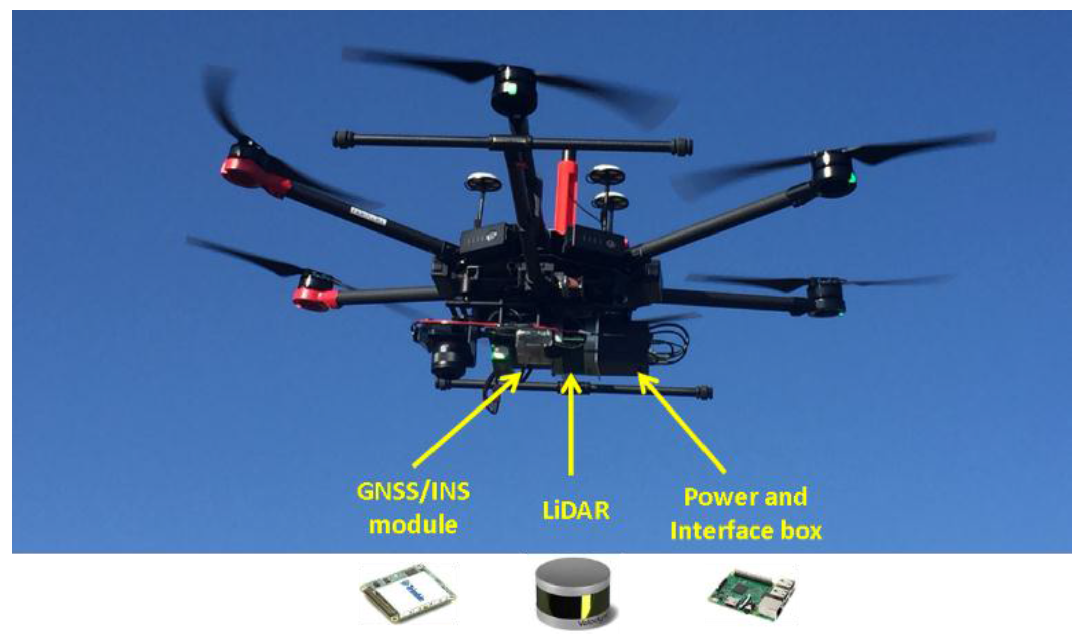
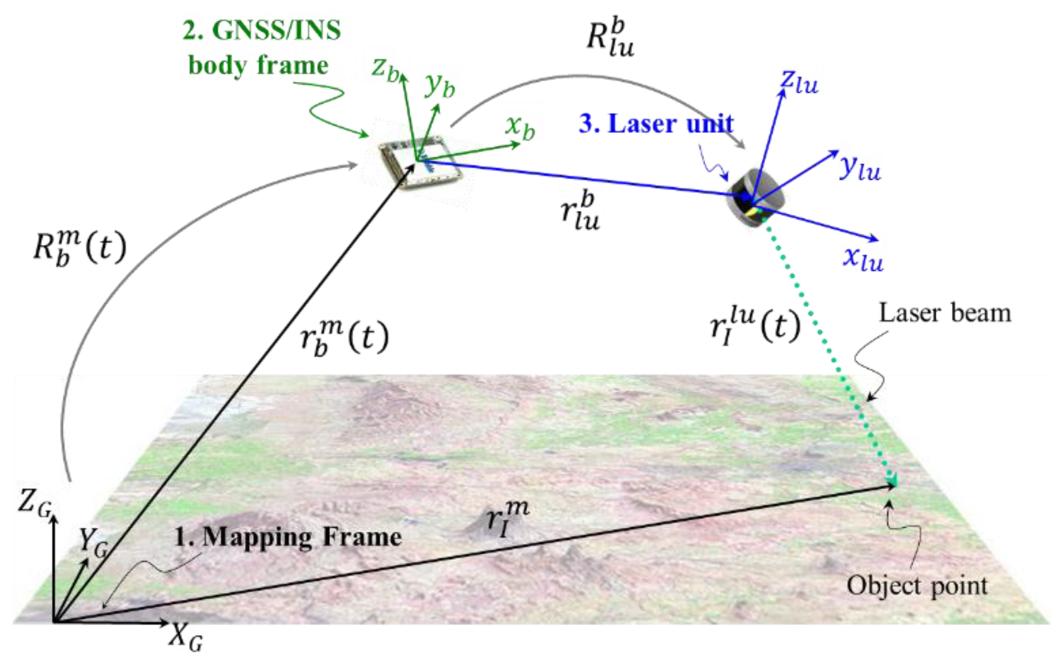
The objective of this section is to derive a mathematical formulation that shows the impact of biases in the mounting parameters on the coordinates of points along planar features with different orientations. This analysis can further aid the development of an optimal/minimal flight and target configuration for calibration. Note that planar features are used specifically for this analysis as they facilitate the observation of positional deformations in one direction at a time, i.e., the effect in the direction normal to the plane. For simplifying the bias impact analysis without any loss of generality, we make several assumptions. Firstly, the IMU is mounted on the UAV with its X- and Y-axes aligned along the starboard and flight line directions, respectively. The IMU is assumed to be perfectly vertical, i.e., the Z-axis of the IMU body frame is assumed to be perfectly aligned with the vertical direction of the mapping frame. Also, we assume that the flight line directions are either from South-to-North ($\kappa =0°$) or from North-to-South ($\kappa =180°$). These assumptions facilitate the decision as to whether the impact is along/across the flight line and vertical directions. As a result, the rotation matrix $R_b^m\left(t\right)$ would be given by Equation (3), where the top and bottom signs are for S-N and N-S flight line directions, respectively. 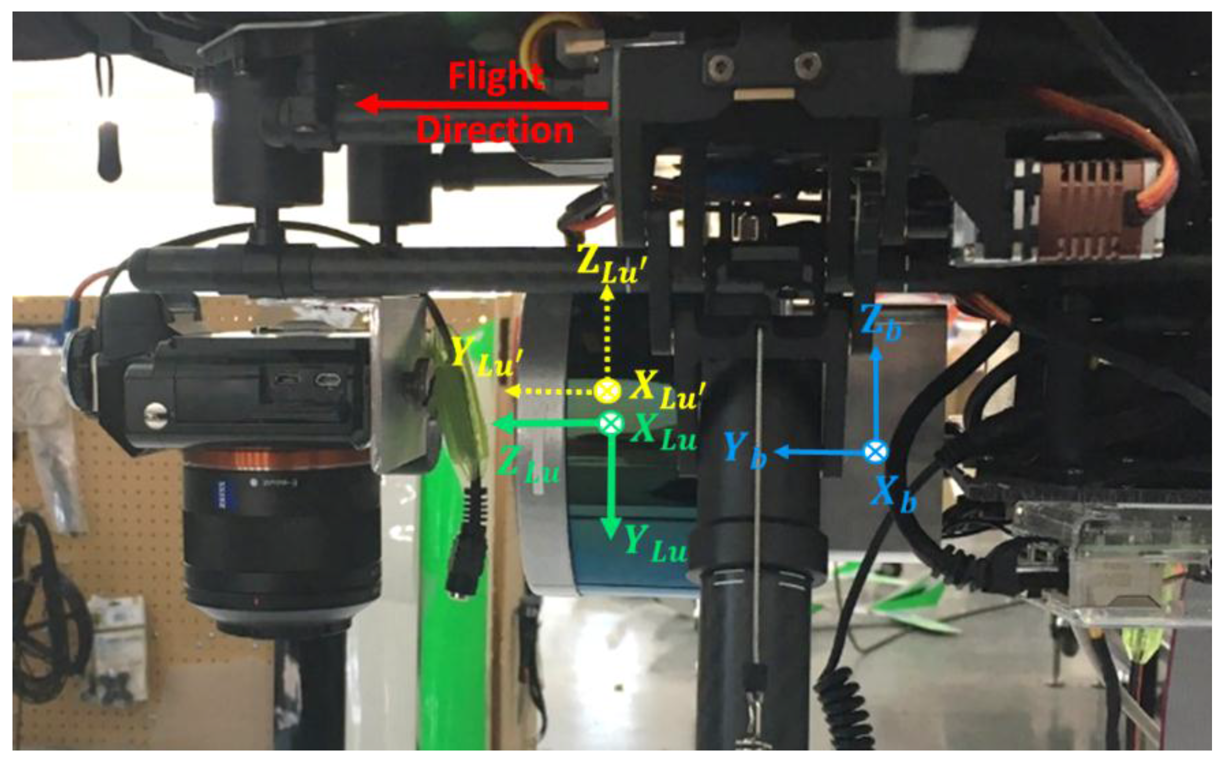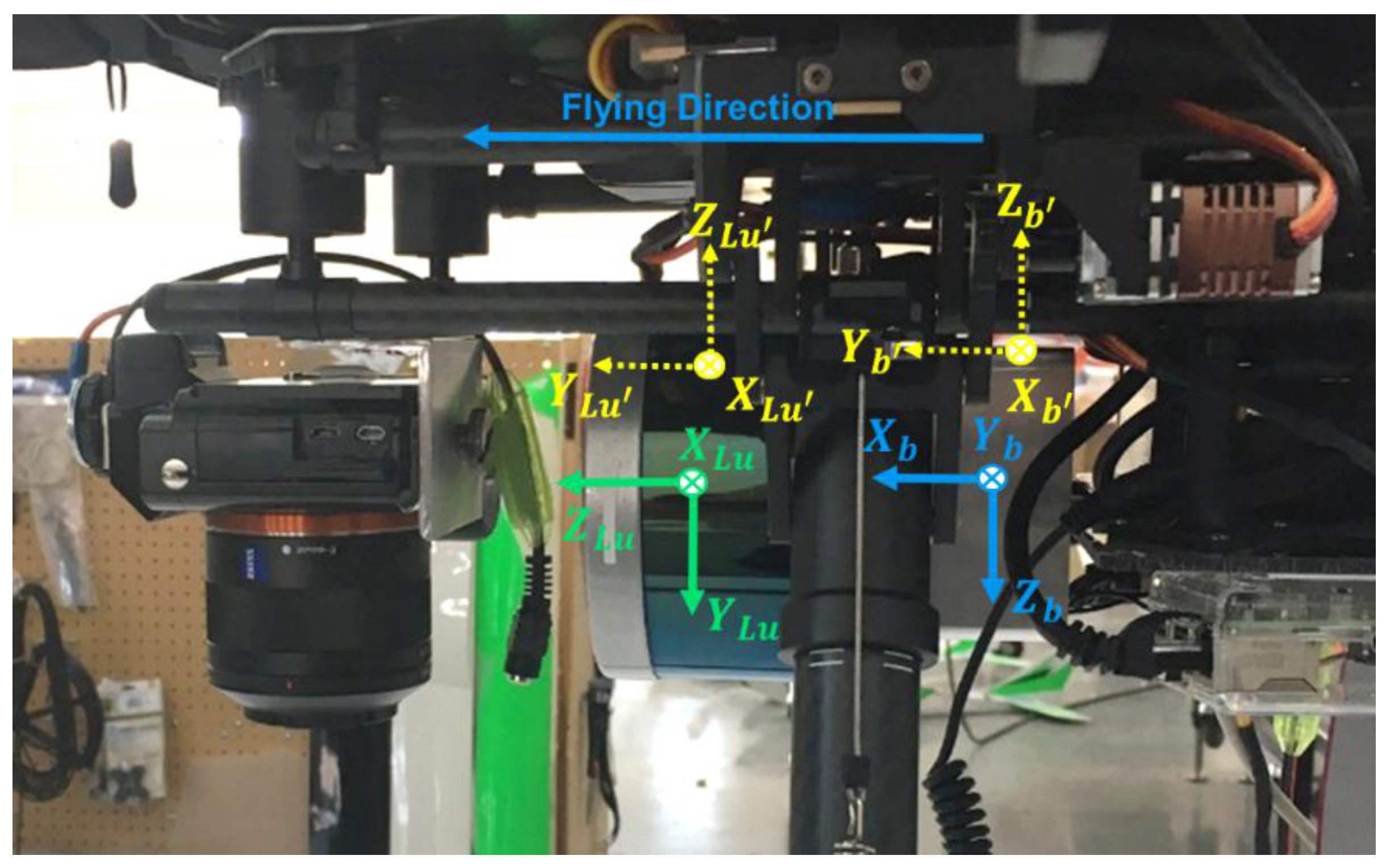In order to generalize the analysis regardless of the orientation of the LiDAR unit relative to the IMU body frame, Equation (1) is slightly modified by introducing a virtual LiDAR unit frame, $L{u}^{\prime }$, which is almost aligned with the IMU body frame. This facilitates the decision as to whether the impact is along/across the flight line and vertical directions. Moreover, the use of a virtual LiDAR unit frame also prevents gimbal lock in the mounting parameter estimation. This modification is implemented by expressing the term $R_{Lu}^b$ in Equation (1) as: $R_{Lu}^b=R_{L{u}^{\prime }}^b R_{Lu}^{L{u}^{\prime }}$, where $R_{Lu}^{L{u}^{\prime }}$ is defined according to the laser scanner unit alignment relative to the IMU. The modified LiDAR point positioning is given by Equation (4). The laser unit coordinate system for the LiDAR unit alignment on the UAV platform used in this system and the assumed IMU body frame coordinate system (with X, Y, Z-axes along starboard, forward and up directions, respectively) are shown in Figure 5.

$$R_b^m\left(t\right)=\left[\begin{array}{ccc}\pm 1& 0& 0\\ 0& \pm 1& 0\\ 0& 0& 1\end{array}\right]$$

(3)

$$r_I^m=r_b^m\left(t\right)+R_b^m\left(t\right) r_{Lu}^b+R_b^m\left(t\right) R_{L{u}^{\prime }}^b R_{Lu}^{L{u}^{\prime }} r_I^{Lu}\left(t\right)$$

(4)

Since the virtual LiDAR unit frame is almost aligned with the IMU body frame, it results in small values for the differential angular boresight parameters ($\Delta \omega$, $\Delta \varphi$, $\Delta \kappa$) relating the two frames. So, the matrix, $R_{L{u}^{\prime }}^b$ can be written as shown in Equation (5), using the small angle approximations. 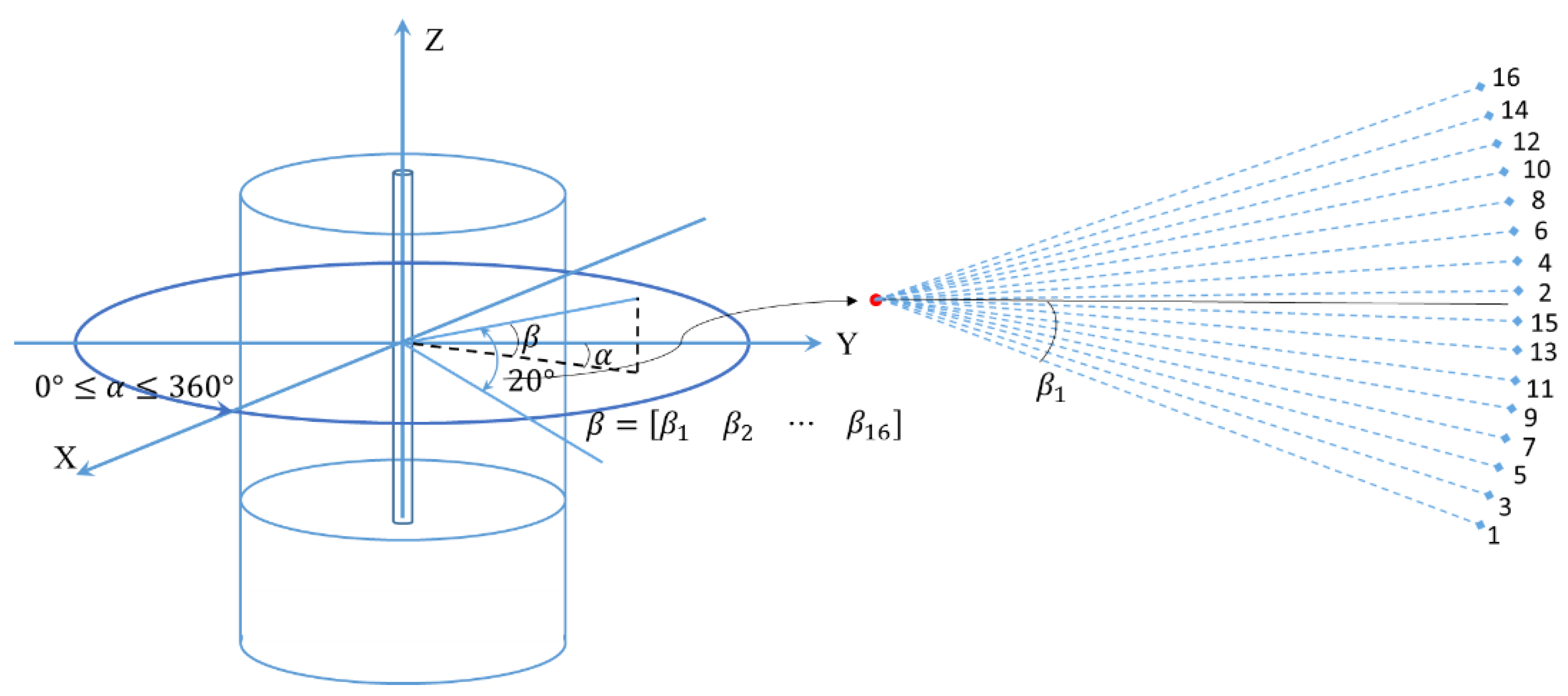Here, $\Delta \omega$, $\Delta \varphi$, $\Delta \kappa$ denote the rotation around the X, Y, Z-axes of the IMU body frame (i.e., across flight, along flight and vertical directions), respectively. Hence, these parameters denote the boresight pitch, roll and heading angles, respectively. The point coordinates relative to the virtual LiDAR unit frame, as derived using the nominal value for $R_{Lu}^{L{u}^{\prime }}=R_{\omega }\left(90°\right) R_{\varphi }\left(0°\right) R_{\kappa }\left(0°\right)$ according to Figure 5, are given by Equations (6a) and (6b) in terms of the flying height, $H\pm \Delta h$ and scan angles $\left(\alpha \mathrm{and}\beta \right)$. 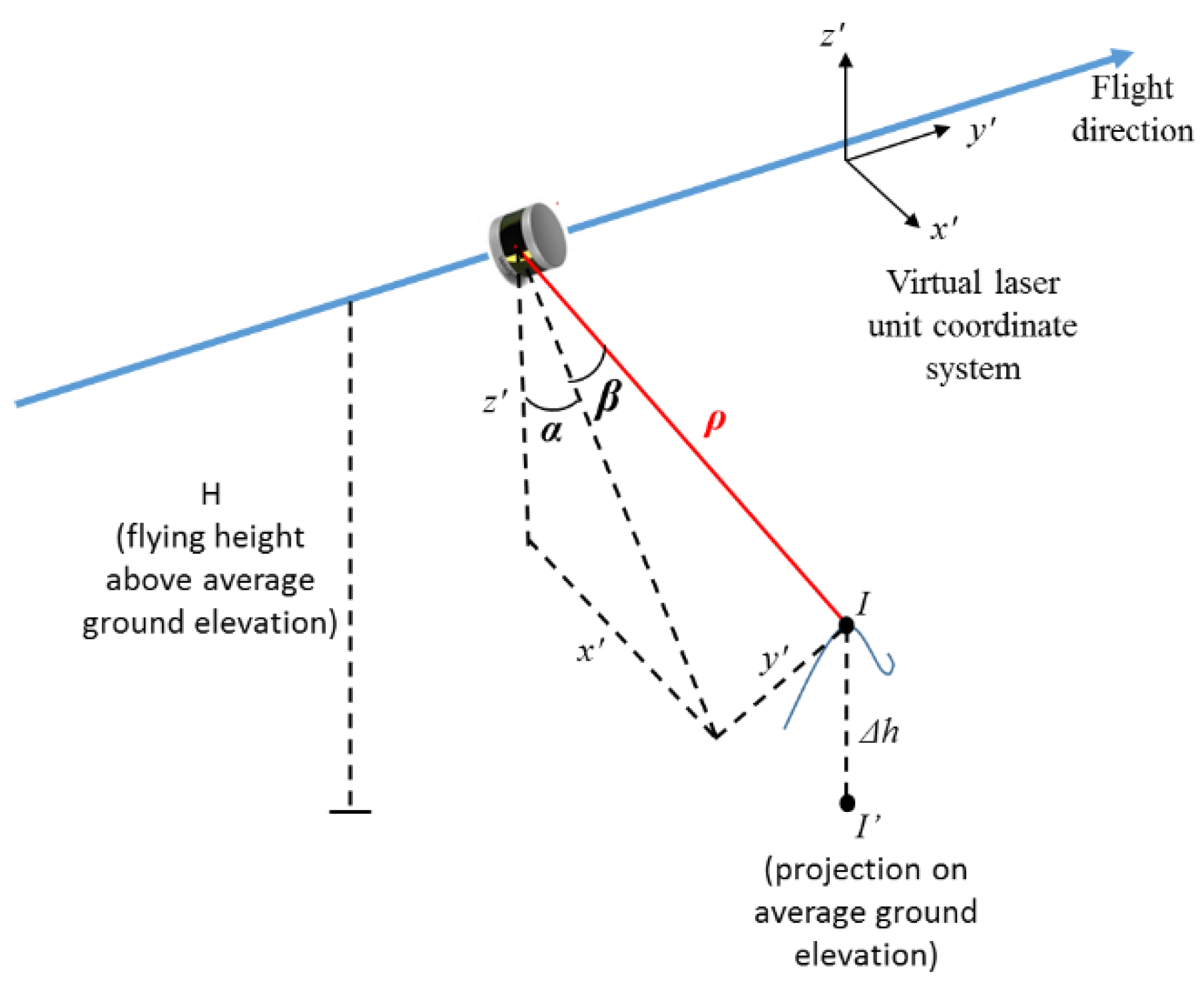These coordinates ($x^{\prime }, y^{\prime }, z^{\prime })$ also denote the location of a point with respect to the virtual LiDAR unit frame, which is almost parallel to the IMU body frame. The schematic illustration of these symbolic notations are depicted in Figure 6 for a UAV-based LiDAR system. Substituting Equations (5) and (6) in Equation (4), we get the revised form of the LiDAR point positioning equation, as given in Equation (7), where $\Delta X$, $\Delta Y$, $\Delta Z$ are the lever-arm offset parameters of the LiDAR unit frame relative to the IMU body frame. Now, the impact of the presence of bias in the system mounting parameters can be analyzed by differentiating Equation (7) with respect to the system mounting parameters. This is given by Equation (8).

$$R_{L{u}^{\prime }}^b=\left[\begin{array}{ccc}1& -\Delta \kappa & \Delta \varphi \\ \Delta \kappa & 1& -\Delta \omega \\ -\Delta \varphi & \Delta \omega & 1\end{array}\right]$$

(5)

$$r_I^{L{u}^{\prime }}\left(t\right)=R_{Lu}^{L{u}^{\prime }}{r}_I^{Lu}\left(t\right)=\left[\begin{array}{c}{x}^{\prime }\\ y^{\prime }\\ z^{\prime }\end{array}\right]=R_{Lu}^{L{u}^{\prime }}\left[\begin{array}{c}\rho \cos \beta \sin \alpha \\ \rho \cos \beta \cos \alpha \\ \rho \sin \beta \end{array}\right]=\left[\begin{array}{c}\rho \cos \beta \sin \alpha \\ \rho \sin \beta \\ -\rho \cos \beta \cos \alpha \end{array}\right]$$

(6a)

$$\left[\begin{array}{c}{x}^{\prime }\\ y^{\prime }\\ z^{\prime }\end{array}\right]=\left(H\pm \Delta h\right)\left[\begin{array}{c}\tan \alpha \\ \frac{\tan \beta }{\cos \alpha }\\ -1\end{array}\right]\left(\mathrm{since}{z}^{\prime }=-\rho \cos \beta \cos \alpha =-\left(H\pm \Delta h\right)\right)$$

(6b)

$$r_I^m=r_b^m\left(t\right)+R_b^m\left(t\right)\left[\begin{array}{c}\Delta X\\ \Delta Y\\ \Delta Z\end{array}\right]+R_b^m\left(t\right)\left[\begin{array}{ccc}1& -\Delta \kappa & \Delta \varphi \\ \Delta \kappa & 1& -\Delta \omega \\ -\Delta \varphi & \Delta \omega & 1\end{array}\right]\left[\begin{array}{c}{x}^{\prime }\\ y^{\prime }\\ z^{\prime }\end{array}\right]$$

(7)

$$\delta r_I^m\left(\delta \Delta X, \delta \Delta Y, \delta \Delta Z, \delta \Delta \omega , \delta \Delta \varphi , \delta \Delta \kappa \right)=\left[\begin{array}{c}\pm \delta \Delta X\\ \pm \delta \Delta Y\\ \delta \Delta Z\end{array}\right]+\left[\begin{array}{c}\pm z^{\prime } \delta \Delta \varphi \mp y^{\prime } \delta \Delta \kappa \\ \mp z^{\prime } \delta \Delta \omega \pm x^{\prime } \delta \Delta \kappa \\ y^{\prime } \delta \Delta \omega -x^{\prime } \delta \Delta \varphi \end{array}\right]$$

(8)

The bias impact can be analyzed thoroughly by isolating the terms in Equation (8) corresponding to the impact of bias in each of the mounting parameters for each of the mapping frame coordinates—$X_m$, $Y_m$ and $Z_m$, representing the coordinates across flying direction, along flying direction and vertical direction, respectively—as given in

Table 1. Impact of bias in each of the mounting parameters on 3D point coordinates.

Bias in System Parameters	$\mathit{\delta }{\mathit{X}}_{\mathit{m}}$	$\mathit{\delta }{\mathit{Y}}_{\mathit{m}}$	$\mathit{\delta }{\mathit{Z}}_{\mathit{m}}$
$\mathit{\delta }\mathbf{\Delta }\mathit{X}$	$\pm \delta \Delta X$	$0$	$0$
$\mathit{\delta }\mathbf{\Delta }\mathit{Y}$	$0$	$\pm \delta \Delta Y$	$0$
$\mathit{\delta }\mathbf{\Delta }\mathit{Z}$	$0$	$0$	$\delta \Delta Z$
$\mathit{\delta }\mathbf{\Delta }\mathit{\omega }$	$0$	$\mp z^{\prime } \delta \Delta \omega$	$y^{\prime } \delta \Delta \omega$
$\mathit{\delta }\mathbf{\Delta }\mathit{\varphi }$	$\pm z^{\prime } \delta \Delta \varphi$	$0$	$-x^{\prime } \delta \Delta \varphi$
$\mathit{\delta }\mathbf{\Delta }\mathit{\kappa }$	$\mp y^{\prime } \delta \Delta \kappa$	$\pm x^{\prime } \delta \Delta \kappa$	$0$

.

Table 1 can now be used to assess the impact of each bias for planar surfaces in different orientations—vertical planes parallel to flight direction, vertical planes perpendicular to flight direction and horizontal planes)—thus indicating the impact across flight direction, along flight direction and vertical direction, respectively.

Impact of Bias in Lever-arm component across the flying direction $\left(\mathbf{\Delta }\mathit{X}\right)$:

The introduced shift across the flying direction $\left(\pm \mathsf{\delta }\Delta X\right)$ is flying direction dependent and does not depend on the location of the point in question relative to the virtual laser unit coordinate system. As a result, its impact will be visible in case of having vertical planes parallel to the flying direction scanned from two flight lines in opposite directions.

Impact of Bias in Lever-arm component along the flying direction $\left(\mathbf{\Delta }\mathit{Y}\right)$:

The introduced shift along the flying direction $\left(\pm \mathsf{\delta }\Delta Y\right)$ is flying direction dependent and does not depend on the location of the point in question relative to the virtual laser unit coordinate system. Again, it would impact vertical planes perpendicular to the flying direction scanned from two flight lines in opposite directions.

Impact of Bias in Lever-arm component in the vertical direction $\left(\mathbf{\Delta }\mathit{Z}\right)$:

The introduced shift in the vertical direction $\left(\mathsf{\delta }\Delta Z\right)$ is flying direction independent and does not depend on the location of the point in question relative to the virtual laser unit coordinate system. As a result, the entire point cloud would be shifted in the vertical direction by the same amount. So, this bias would not affect planes at any orientation for any flight line configuration.

Impact of Bias in Boresight Pitch $\left(\mathbf{\Delta }\mathit{\omega }\right)$:

A bias in this component $\left(\mathsf{\delta }\Delta \omega \right)$ will cause shifts along the flying direction as well as in the vertical direction. The impact of boresight pitch bias along the flying direction $\left(\mp z^{\prime } \delta \Delta \omega =\pm \left(H\pm \Delta h\right) \delta \Delta \omega \right)$ is flying direction dependent and its magnitude depends on the height ($z^{\prime }$) of the point in question relative to the virtual laser unit coordinate system. This impact would be visible in case of a planar feature perpendicular to the flying direction being scanned by flight lines in opposite directions. The impact of boresight pitch bias in the vertical direction $\left(y^{\prime } \delta \Delta \omega \right)$ would be manifested in horizontal planes. The magnitude of this impact depends on the $y^{\prime }$-coordinate of the point in question. So, this impact would be visible even in case of a single flight line capturing a horizontal planar feature as long as there is a significant variation in the $y^{\prime }$-coordinate at a given location within such a plane, i.e., if the same portion of the plane is scanned by the laser unit while being at different locations.

Since a bias in lever arm $\Delta Y$ also causes shifts along the flying direction, there is a need to decouple the impacts so as to estimate both these biases accurately. Due to the impact of boresight pitch bias in the vertical direction in addition to the impact along flying direction, it would aid in naturally decoupling $\delta \Delta \omega$ and $\delta \Delta Y$, provided there is a significant $y^{\prime }$-coordinate variability. But, the $y^{\prime }$-coordinate variation could be reduced depending on the nature of the targets used or the sensor configuration. In this case, the $y^{\prime }$-coordinate variability is limited by the relatively narrow vertical FOV of the LiDAR unit (±10°), thus making it insufficient to eliminate the correlation. In such cases, there is a need to have a significant variation in the value of $\left(H\pm \Delta h\right)$ in order to decouple the impacts of $\delta \Delta Y$ and $\delta \Delta \omega$ so as to estimate both these biases accurately. This can be achieved by one of the following ways:

• Two different flying heights: The shift caused along the flight direction by the bias $\delta \Delta \omega$ will vary depending on the flying height, whereas the shift due to the bias $\delta \Delta Y$ will be constant for any flying height. Thus, the two biases can be derived accurately using flight lines at different flying heights.
• Variation in target height w.r.t. flying height: In case of flight lines at the same flying height, a variation in the height of points along a target primitive would result in varying shifts. The amount of variation required depends on the flying height, i.e., $H\pm \Delta h=H\left(1\pm \frac{\Delta h}{H}\right)$. So, the higher the value of $\frac{\Delta h}{H}$ for a given flying height, the better the estimation accuracy of $\Delta Y$ and $\Delta \omega$ will be. A high variation in $\frac{\Delta h}{H}$ can be achieved either by having vertical planes at different heights or with a significant variation in the heights along given targets.

Impact of Bias in Boresight Roll $\left(\mathbf{\Delta }\mathit{\varphi }\right)$:

A bias in this component ($\delta \Delta \varphi$) will cause shifts across the flying direction as well as in the vertical direction. The impact of this bias across the flying direction $\left(\pm z^{\prime } \delta \Delta \varphi =\mp \left(H\pm \Delta h\right) \delta \Delta \varphi \right)$ is flying direction dependent and its magnitude depends on the height ($z^{\prime }$) of the point in question relative to the virtual laser unit coordinate system. This bias would impact vertical planes parallel to the flying direction scanned from two flight lines in opposite directions. 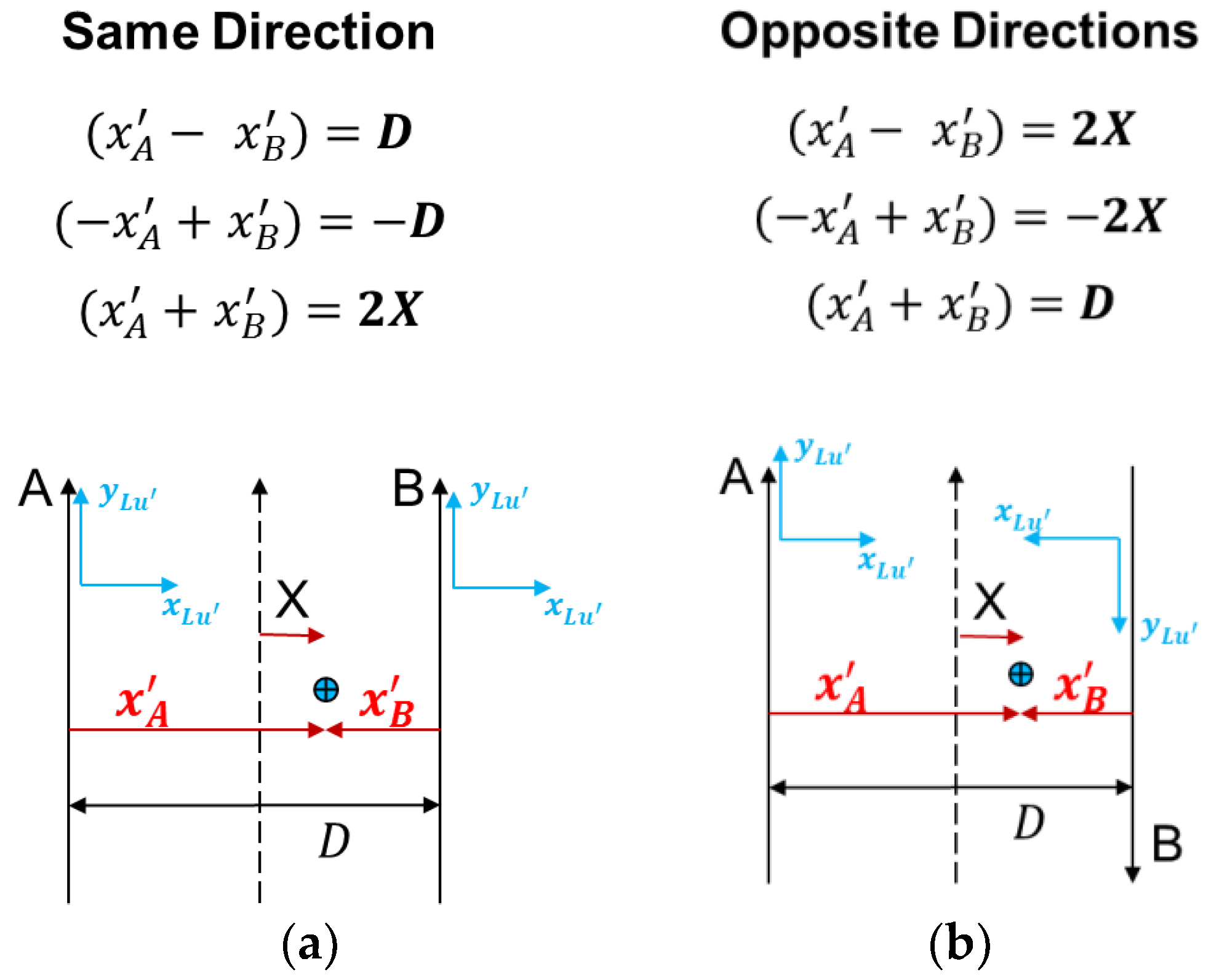The impact of this bias in the vertical direction $\left(-x^{\prime }\delta \Delta \varphi \right)$ is flying direction dependent (since $x^{\prime }$-coordinates will change signs depending on the flying direction, as shown in Figure 6) and its magnitude depends on the $x^{\prime }$-coordinate of the point in question. The resultant discrepancy in the Z-coordinate on combining two tracks in the same and opposite directions are given by Equations (9) and (10), respectively, according to Figure 7. Here, $D_{AB}$ denotes the lateral distance between the two tracks and $X$ denotes the distance of the point in question from the line bisecting the lateral distance between the two flight lines. The analysis reveals that this bias would cause a discrepancy for horizontal planes scanned from two flight lines in the same direction depending on the lateral distance between the tracks. On the other hand, for two tracks in opposite directions, the discrepancy would depend on the lateral location of the planar patch of interest relative to the bisecting direction between the tracks.

$$\mathrm{Same} \mathrm{direction}: \delta Z_{m_A}-\delta {Z_m}_B=\left(-x_A^{\prime }+x_B^{\prime }\right) \delta \Delta \varphi =-D_{AB}\delta \Delta \varphi$$

(9)

$$\mathrm{Opposite} \mathrm{directions}: \delta {Z_m}_A-\delta {Z_m}_B=\left(-x_A^{\prime }+x_B^{\prime }\right) \delta \Delta \varphi =-2X\delta \Delta \varphi$$

(10)

Since a bias in lever arm $\Delta X$ also causes shifts across the flying direction, there is a need to decouple the impacts of $\delta \Delta X$ and $\delta \Delta \varphi$ so as to estimate both these biases accurately. Due to the impact of boresight roll bias in the vertical direction in addition to the impact across flying direction, it would aid in naturally decoupling $\delta \Delta \varphi$ and $\delta \Delta X$, provided there are planar patches scanned from flight lines in the same direction with sufficient lateral separation and also, some planar patches located at a significantly high lateral distance from the flight lines. However, in the case of the unavailability of such planar patches located at a high lateral distance, the decoupling of the two parameters can be achieved by ensuring a significant variation in the value of $\left(H\pm \Delta h\right)$. This can be achieved by one of the following ways:

• Two different flying heights: The shift caused along the flying direction by the bias $\delta \Delta \varphi$ will vary depending on the flying height, whereas the shift due to the bias $\delta \Delta X$ will be constant for any flying height. Thus, the two biases can be derived accurately using flight lines at different flying heights.
• Variation in target height w.r.t. flying height: In case of flight lines at the same flying height, a variation in the height of points along a target primitive would result in varying shifts. The amount of variation required depends on the flying height, i.e., $H\pm \Delta h=H\left(1\pm \frac{\Delta h}{H}\right)$. So, the higher the value of $\frac{\Delta h}{H}$ for a given flying height, the better the estimation accuracy of $\Delta X$ and $\Delta \varphi$ will be.

Impact of Bias in Boresight Heading $\left(\mathbf{\Delta }\mathit{\kappa }\right)$:

A bias in this component $\left(\delta \Delta \kappa \right)$ will cause shifts across and along the flying direction. The impact of this bias across the flying direction $\left(\mp y^{\prime } \delta \Delta \kappa \right)$ is dependent on the $y^{\prime }$-coordinate variability. So, this would cause a discrepancy for vertical planes parallel to the flying direction for a single track. Moreover, the discrepancy on combining two tracks in same or opposite directions would depend on the $\pm y^{\prime }$ variability within the points comprising the planes.

The impact of this bias along the flying direction $\left(\pm x^{\prime } \delta \Delta \kappa \right)$ is flying direction independent since the sign change of $x\prime$-coordinate on flight direction change is nullified by the presence of dual sign in the term. Also, the magnitude of this impact is $x\prime$-coordinate dependent. This bias would induce a discrepancy in case of vertical planes perpendicular to the flying direction scanned from two flight lines in the same/opposite directions depending on the lateral distance between the tracks, as given by Equations (11) and (12). For the UAV system used in this study, the impact along flying direction will be more pronounced than the impact across flying direction since the LiDAR unit is scanning with the laser beams rotating 360° around the $y^{\prime }$-axis, thus resulting in a high $x^{\prime }$-coordinate variability. However, the $y^{\prime }$-coordinate variability is limited by the total vertical FOV of ±10° of the Velodyne VLP-16 Puck Hi-Res unit.

$$\mathrm{Same} \mathrm{direction}: \delta {Y_m}_A-\delta {Y_m}_B=\left(x_A^{\prime }-x_B^{\prime }\right)\delta \Delta \kappa =D_{AB}\delta \Delta \kappa$$

(11)

$$\mathrm{Opposite} \mathrm{directions}: \delta {Y_m}_A-\delta {Y_m}_B=\left(x_A^{\prime }+x_B^{\prime }\right)\delta \Delta \kappa =D_{AB}\delta \Delta \kappa$$

(12)

Throughout the previous discussion, we dealt with a system where the LiDAR unit coordinate system is not aligned with IMU body frame but it was dealt with by using a virtual laser unit frame. However, the X, Y, Z-axes of the IMU body frame were assumed to be aligned along the starboard, forward and up directions. For other generic situations where the IMU body frame is not aligned in such a manner, we can also account for that by introducing a virtual IMU body frame. For such cases, the LiDAR equation will be modified to result in Equation (13). Here, $R_{b^{\prime }}^b$ is a fixed rotation depending on the alignment of the actual IMU body frame relative to the UAV vehicle frame. Hence, this modification renders the current bias impact analysis indifferent to the LiDAR unit and IMU body frame alignment within the platform.

$$r_I^m=r_b^m\left(t\right)+R_b^m\left(t\right) R_{b^{\prime }}^b r_{Lu}^{b^{\prime }}+R_b^m\left(t\right) R_{b^{\prime }}^b R_{L{u}^{\prime }}^{b^{\prime }} R_{Lu}^{L{u}^{\prime }} r_I^{Lu}\left(t\right)$$

(13)

3.3. Optimal Flight Line Configuration for Calibration

Based on the above discussion, the following comments can be made regarding an optimal flight configuration for calibration:

• The lever arm $\Delta X$ can be estimated using opposite flight lines while scanning vertical planar features parallel to the flight direction.
• The lever arm $\Delta Y$ can be estimated using opposite flight lines while scanning vertical planar features perpendicular to the flight direction.
• The lever arm $\Delta Z$ for a given spinning multi-beam laser scanner can be estimated only using vertical control, which can be in the form of horizontal planar patches.
• The boresight pitch $\Delta \omega$ can be estimated using opposite flight lines along with another flight line at a different height while scanning horizontal planar features and vertical planar features perpendicular to the flight direction. Another alternative for having a flight line at different flying height is to have vertical planar features whose extent in the vertical direction is significant w.r.t. the flying height or having vertical planar patches at different heights.
• The boresight roll $\Delta \varphi$ can be estimated using opposite flight lines along with another flight line at a different height while scanning horizontal planar features and vertical planar features parallel to the flight direction. Another alternative for having a flight line at different flying height is to have vertical planar features with significant height w.r.t. the flying height or having vertical planar patches at different heights. Additionally, increasing the lateral distance between the tracks and between horizontal patches and the tracks would improve the boresight roll estimation.
• The boresight heading $\Delta \kappa$ can be estimated by scanning vertical planes from two flight lines in the same direction with a significant lateral separation between them. This configuration would eliminate any discrepancies caused by lever-arm components.

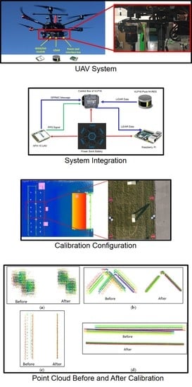
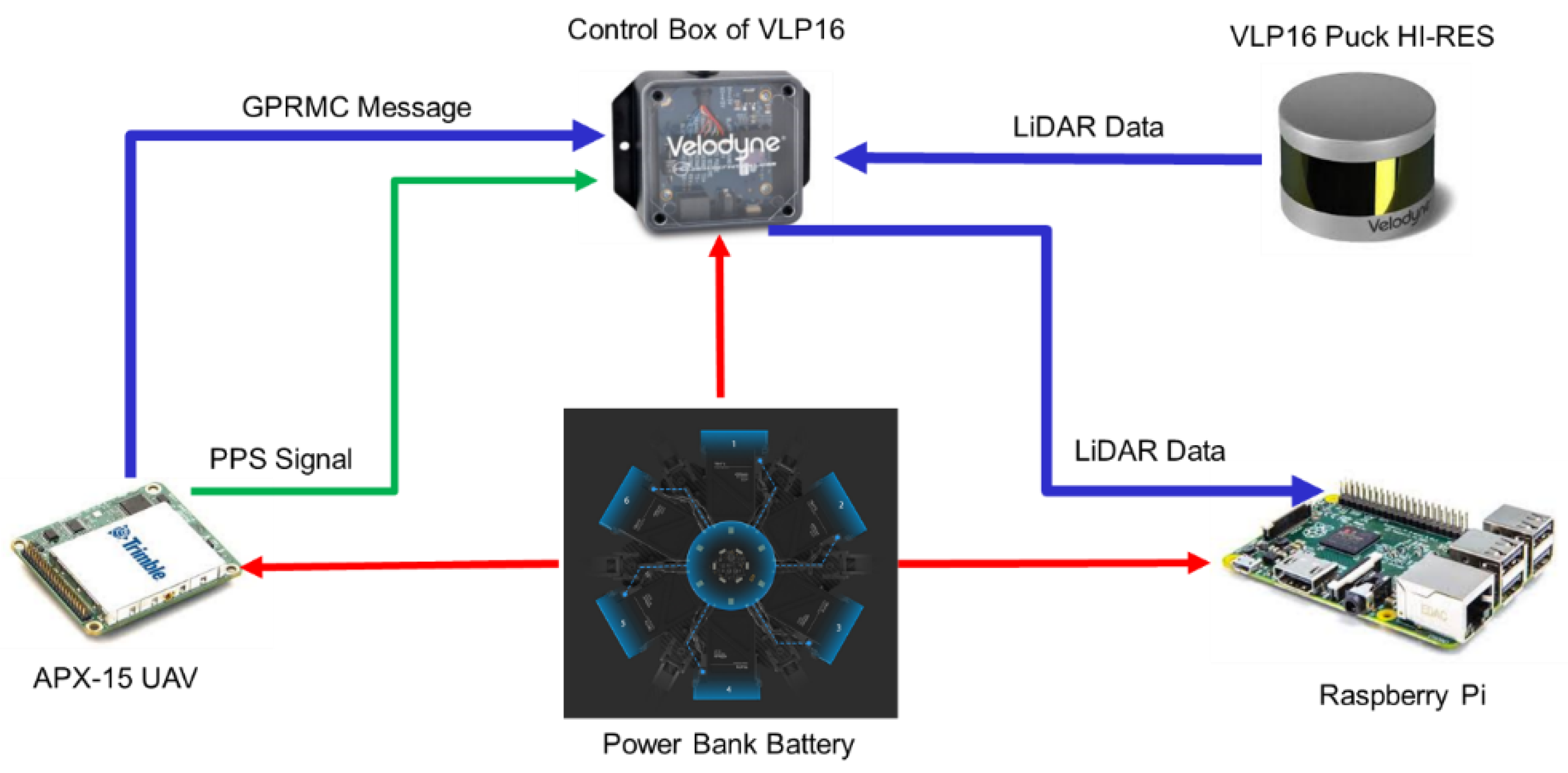
3.4. Calibration Strategy for UAV-Based LiDAR System

In this section, we propose a strategy to calibrate the mounting parameters of the LiDAR unit with respect to the onboard GNSS/INS unit using geometric tie features (e.g., planar and linear/cylindrical features). The conceptual basis for LiDAR system calibration is to minimize the discrepancies among conjugate linear and/or planar features obtained from different flight lines. Owing to the irregular distribution of LiDAR points, conjugate point pairs cannot be used since there is no accurate point-to-point correspondence. So, conjugate linear/cylindrical and planar features, such as building façades, ground patches, light poles and lane markers, are used and these can be directly extracted from overlapping areas within the flight lines. After collecting data from several flight lines, a 3D point cloud relative to a global reference frame will be derived using the GNSS/INS unit position and orientation and initial estimates for the mounting parameters. Then, conjugate features are identified and extracted from the reconstructed point cloud. 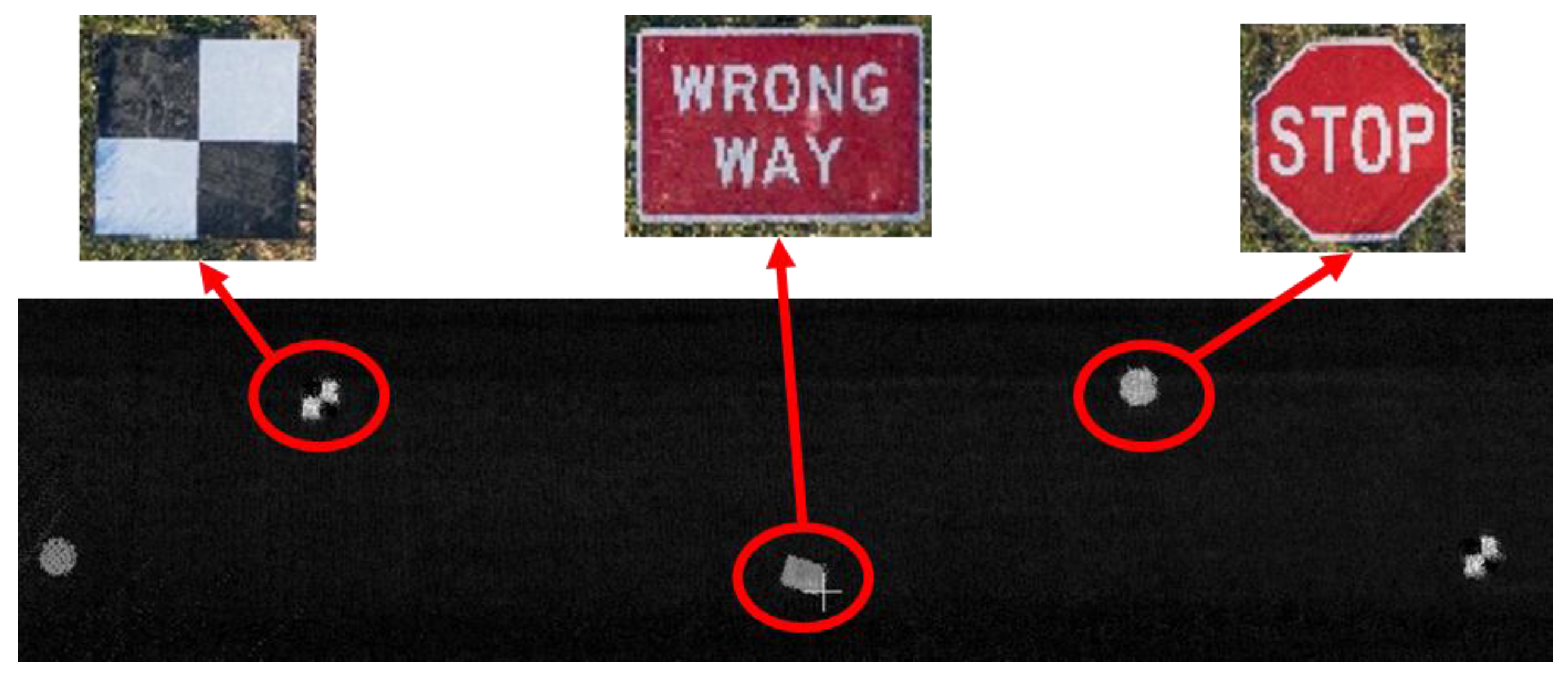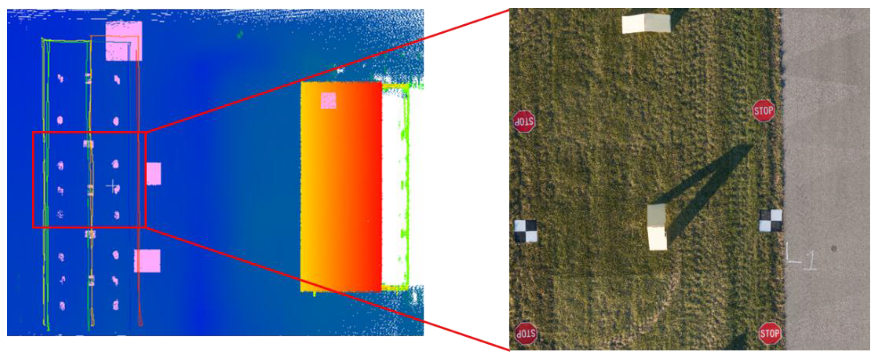Finally, an iterative LiDAR system calibration with weight modification [18] is proposed to derive the mounting parameters based on the minimization of normal distance between conjugate features. However, conjugate feature extraction from several flight lines could be time-consuming and inefficient, especially when the initial estimates for mounting parameters used to reconstruct the 3D point cloud are considerably inaccurate. To facilitate automated identification of conjugate features in such cases, specifically designed calibration boards covered by highly reflective surfaces, that could be easily deployed and set up in outdoor environments, are used in this study. More specifically, various traffic signs (75 cm wide Stop signs, 90 cm × 60 cm Wrong Way signs and 60 cm × 60 cm checkerboard targets) are used as highly reflective boards. The highly reflective boards can be easily identified from intensity data, as shown in Figure 8, where the points belonging to these boards exhibit higher intensity values compared to other LiDAR points. First, a pre-defined threshold is set to extract high-intensity points. To avoid the extraction of high-intensity points belonging to objects other than these boards, an approximate pre-set region is set as seed points for each board. Then, a distance-based region growing technique is adopted to group the high intensity board returns. Finally, a plane-fitting is done for these points and the points lying within a normal distance threshold from the best-fitting plane are extracted. Other planar features, such as ground patches or wall patches, can be extracted by defining two diagonally opposite corners and selecting the points lying within a buffer bounding box. The bounding box is constructed around the planar feature of interest by adding a buffer value (in X, Y and Z directions) to the coordinates of diagonally opposite corners. Again, a plane-fitting is done for the points contained inside the box and the ones lying within a normal distance threshold from the best-fitting plane are extracted. Linear/cylindrical features can also be used for calibration and they are extracted by specifying the two end points for each feature. A buffer radius is set to define a cylinder around the linear feature of interest. Then, a line-fitting is done for the points lying within this cylindrical buffer and finally, the points that lie within a normal distance threshold from the best-fitting line are extracted. Note that the buffer values for linear/planar feature extraction are determined based on the accuracy of initial estimates of the mounting parameters.

The mounting parameters that are derived from calibration are the lever arm $\left(\Delta X, \Delta Y\right)$ and boresight angles $\left(\Delta \omega , \Delta \varphi , \Delta \kappa \right)$ for the LiDAR unit. The lever arm $\Delta Z$ for the LiDAR unit cannot be estimated in the calibration procedure since any change in $\Delta Z$ will not introduce discrepancies among the different versions of the same feature captured from different flight lines. It would only result in a shift of the point cloud in the vertical direction as a whole. It is either manually measured or determined using vertical control (such as, horizontal planar patches with known elevation) and fixed during the calibration procedure.

Finally, the mounting parameters of each sensor are derived by minimizing the discrepancies between non-conjugate point pairings among conjugate features in overlapping flight lines. In case of a planar feature, the discrepancy arising from each non-conjugate point pair would consist of a non-random component lying along the planar surface. Hence, a modified weight is applied to the point pair so as to retain only the component of the discrepancy lying along the direction normal to the planar surface. Similarly, in case of a linear/cylindrical feature, a modified weight is applied so as to nullify the component of discrepancy along the direction of the feature. The modified weight is determined according to the direction of the planar/linear feature as obtained from the feature parameters derived by a plane/line fitting conducted on the points from the flight line that captures the most number of points belonging to the corresponding feature. A more detailed discussion regarding the theoretical basis for weight modification while using non-conjugate points along corresponding features can be found in Renaudin et al. (2011) [18]. Finally, the mounting parameters for the laser unit can be derived by minimizing the discrepancies among the conjugate features arising from the above-mentioned pairs.

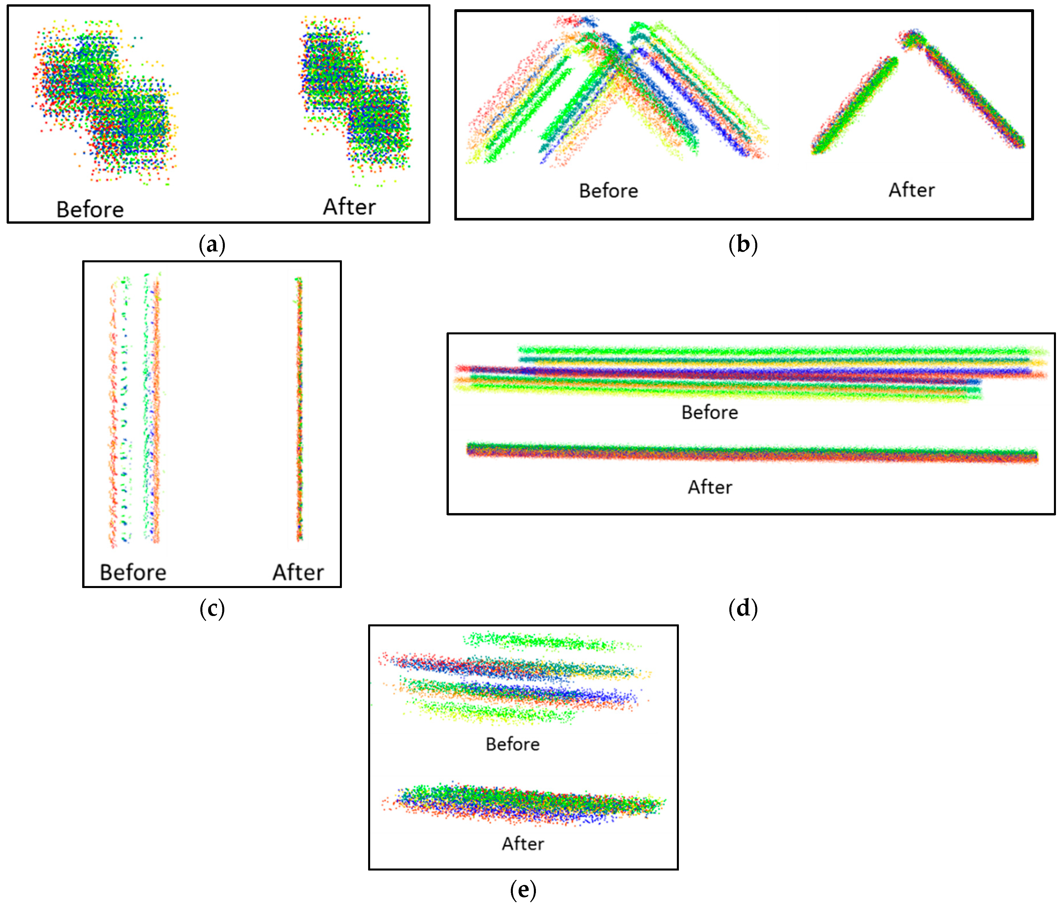
However, when the initial estimate of the mounting parameters is inaccurate, the estimated modified weight matrix would be imprecise which would affect the accuracy of the derived mounting parameters. Hence, this research proposes an iterative calibration procedure. Firstly, the discrepancy among extracted features is minimized to derive mounting parameters through the weight modification process. Then, the points along the extracted features are re-generated using the newly estimated mounting parameters and the discrepancy among conjugate features is minimized again using a newly defined modified weight matrix. The above steps are repeated until the change in the estimates of the mounting parameters is below a predefined threshold. In this study, these stopping criteria are enforced by monitoring the difference between the a-posteriori variance factors after two consecutive iterations of LSA and when the difference is less than 10⁻⁸, the adjustment is deemed complete. Since the a-posteriori variance factor indicates the average accuracy of calibration by quantifying the normal distance of points from best-fitting plane/line for all the extracted features, the threshold of 10⁻⁸ indicates a change of less than 0.01 µm in the overall normal distance, which can be definitely regarded as insignificant.

4. Experimental Results

Having conducted a thorough analysis of the impact of biases in the different mounting parameters of a UAV-based LiDAR system to devise an optimal flight and target configuration and proposed a calibration strategy, we now conduct several experiments to validate the feasibility of the proposed strategy and quality of calibration, followed by an evaluation of the devised optimal configuration based on the standard deviation and correlation matrix for the mounting parameters for various test cases. For the UAV system consisting of a Velodyne VLP-16 Puck Hi-Res LiDAR unit and an APX-15 GNSS/INS unit, we use the LiDAR Error Propagation Calculator developed by Habib et al. (2006) [19] to compute the expected accuracy of point positioning for this system. The calculator suggests an accuracy of 5–6 cm for a flying height of 15–25 m. In this study, the UAV-based LiDAR system is flown with six tracks each at a flying height of 15 m and 25 m with a speed of 1.5 m/s over sixteen specially designed highly reflective boards (75 cm wide Stop signs, 90 cm × 60 cm Wrong Way signs and 60 cm × 60 cm checkerboard targets) and five hut-shaped targets (with two 60 cm × 120 cm planar boards) with their ridges oriented parallel and perpendicular to the flying direction. The average lateral separation between the tracks is 6 m. The two surfaces corresponding to each of these huts are used as planar features for calibration and their ridges are used as conjugate linear features. Additional planar features, such as ground patches, rooftops and building facades, are also used for calibration. The configuration of the tracks and the target primitives (in pink) are shown in Figure 9. For the UAV system used in this study, the X, Y, Z-axes of the IMU body frame are not aligned along the starboard, forward and up directions. Instead the coordinate frames are aligned as shown in Figure 10. So, a virtual IMU body frame defined as per Equation (13) is used. Therefore, we are estimating the mounting parameters relating the virtual IMU and virtual laser unit coordinate systems.

4.1. Single Flying Height

First, a sub-optimal configuration is used to evaluate the theoretical bias impact analysis for the estimation of system parameters. In this case, six flight lines at a single flying height of 15 m are used along with the target primitives lying exactly below the flight lines (the sixteen boards and five hut-shaped targets) and with no significant x’ and z’-coordinate variation. The initial approximations of these mounting parameters and the final results (along with their standard deviations) from the proposed calibration procedure are listed in

Table 2. Mounting parameters of VLP-16 before and after calibration test 1 (the parameter fixed during calibration is shown in red).

VLP-16 LiDAR Unit Mounting Parameters $\left({\mathit{r}}_{\mathit{L}{\mathit{u}}^{\prime }}^{{\mathit{b}}^{\prime }}\right)$ $\left({\mathit{R}}_{\mathit{L}{\mathit{u}}^{\prime }}^{{\mathit{b}}^{\prime }}\right)$
System Parameters	$\Delta \mathit{X}$ (m)	$\mathbf{\Delta }\mathit{Y}$ (m)	$\mathbf{\Delta }\mathit{Z}$ (m)	$\mathbf{\Delta }\mathit{\omega }$ (°)	$\mathbf{\Delta }\mathit{\varphi }$ (°)	$\mathbf{\Delta }\mathit{\kappa }$ (°)
Initial	0	0.02	0	0	0	0
Final	0.0084	−0.0037	0	0.1676	−0.7666	−0.2825
Standard Deviation	0.0168	0.0381	Fixed	0.0797	0.0323	0.0542

. Here, the lever arm $\Delta Z$ for the laser unit is fixed during the calibration procedure. One should note that the magnitude of lever-arm components depend on the physical location of the LiDAR unit with respect to the GNSS/INS unit. In this case, the very close positioning of LiDAR and GNSS/INS units results in the small values for lever-arm components. On the other hand, the standard deviation obtained for these parameters after LSA is a function of the geometry of the flight lines (flight/primitive configuration) and the accuracy of the involved hardware components (GNSS/INS unit and laser scanner and ranging unit). Hence the standard deviation should decrease as the configuration of the flight lines is improved (as clear from the results of other forthcoming tests). As stated before, according to the accuracies of the involved hardware components, the LiDAR Error Propagation Calculator [19] suggests an accuracy of 5–6 cm in point positioning for a flying height of 15–25 m. Hence, the standard deviations of the lever-arm and boresight parameters, as expected, are observed to lie within the accuracy expected according to the hardware components, thus proving the feasibility of the proposed strategy. The correlation matrix for the estimated mounting parameters of the laser unit is also listed in

Table 3. Correlation matrix of mounting parameter estimates from calibration test 1 (the potential high correlation values are shown in red).

System Parameters	$\mathbf{\Delta }\mathit{X}$	$\mathbf{\Delta }\mathit{Y}$	$\mathbf{\Delta }\mathit{Z}$	$\mathbf{\Delta }\mathit{\omega }$	$\mathbf{\Delta }\mathit{\varphi }$	$\mathbf{\Delta }\mathit{\kappa }$
$\mathbf{\Delta }\mathit{X}$	1.0000	0.1258	0.0000	0.1303	$\mathbf{0.6647}$	0.0231
$\mathbf{\Delta }\mathit{Y}$	0.1258	1.0000	0.0000	$\mathbf{0.9905}$	0.0922	0.0296
$\mathbf{\Delta }\mathit{Z}$	0.0000	0.0000	0.0000	0.0000	0.0000	0.0000
$\mathbf{\Delta }\mathit{\omega }$	0.1303	$\mathbf{0.9905}$	0.0000	1.0000	0.0916	0.0263
$\mathbf{\Delta }\mathit{\varphi }$	$\mathbf{0.6647}$	0.0922	0.0000	0.0916	1.0000	0.0351
$\mathbf{\Delta }\mathit{\kappa }$	0.0231	0.0296	0.0000	0.0263	0.0351	1.0000

, which indicates that $\Delta Y$ is highly correlated with $\Delta \omega$ (0.9905). The average accuracy after calibration can be quantified by the square root of the a-posteriori variance factor $({\hat{\sigma }}_o)$, which is 3.12 cm in this case. This is better than the expected accuracy of around 5–6 cm according to the accuracies of the hardware involved and an error propagation calculation.

The high correlation between the system parameters ($\Delta Y$ and $\Delta \omega$) renders the calibration results unreliable. So, we incorporate planar features located at a high lateral separation from the flight lines (ground patches, rooftops and building façade) while still considering flight lines at a single flying height of 15 m. The corresponding mounting parameters and correlation matrix are listed in

Table 4. Mounting parameters of VLP-16 before and after calibration test 2 (the parameter fixed during calibration is shown in red).

VLP-16 LiDAR Unit Mounting Parameters $\left({\mathit{r}}_{\mathit{L}{\mathit{u}}^{\prime }}^{{\mathit{b}}^{\prime }}\right)$ $\left({\mathit{R}}_{\mathit{L}{\mathit{u}}^{\prime }}^{{\mathit{b}}^{\prime }}\right)$
System Parameters	$\mathbf{\Delta }\mathit{X}$ (m)	$\mathbf{\Delta }\mathit{Y}$ (m)	$\mathbf{\Delta }\mathit{Z}$ (m)	$\mathbf{\Delta }\mathit{\omega }$ (°)	$\mathbf{\Delta }\mathit{\varphi }$ (°)	$\mathbf{\Delta }\mathit{\kappa }$ (°)
Initial	0	0.02	$0$	0	0	0
Final	0.0180	−0.0067	$0$	0.1598	−0.6942	−0.2538
Standard Deviation	0.0118	0.0181	$\mathrm{Fixed}$	0.0361	0.0139	0.0438

and

Table 5. Correlation matrix of mounting parameter estimates from calibration test 2 (the potential high correlation values are shown in red).

System Parameters	$\mathbf{\Delta }\mathit{X}$	$\mathbf{\Delta }\mathit{Y}$	$\mathbf{\Delta }\mathit{Z}$	$\mathbf{\Delta }\mathit{\omega }$	$\mathbf{\Delta }\mathit{\varphi }$	$\mathbf{\Delta }\mathit{\kappa }$
$\mathbf{\Delta }\mathit{X}$	1.0000	0.0240	0.0000	0.0141	$\mathbf{0.1025}$	0.0298
$\mathbf{\Delta }\mathit{Y}$	0.0240	1.0000	0.0000	$\mathbf{0.9032}$	0.1390	0.0171
$\mathbf{\Delta }\mathit{Z}$	0.0000	0.0000	0.0000	0.0000	0.0000	0.0000
$\mathbf{\Delta }\mathit{\omega }$	0.0141	$\mathbf{0.9032}$	0.0000	1.0000	0.1775	0.0221
$\mathbf{\Delta }\mathit{\varphi }$	$\mathbf{0.1025}$	0.1390	0.0000	0.1775	1.0000	0.2456
$\mathbf{\Delta }\mathit{\kappa }$	0.0298	0.0171	0.0000	0.0221	0.2456	1.0000

, respectively. The standard deviation of all the estimated parameters can be seen to have reduced as compared to the previous case. Moreover, the correlation matrix indicates a reduction in the correlation between $\Delta Y$ and $\Delta \omega$ from 0.9905 to 0.9032 and the correlation between $\Delta X$ and $\Delta \varphi$ is also reduced from 0.6647 to 0.1025. These reductions can be attributed to the variation in z’ and x’-coordinates, as derived in the theoretical bias impact analysis. The correlation between all the other parameters has also decreased, thus proving the improvement in calibration results. The average accuracy after calibration as quantified by the square root of the a-posteriori variance factor $({\hat{\sigma }}_o)$ is 2.22 cm in this case, which is also less than the previous case of 3.12 cm.

4.2. Multiple Flying Heights

Finally, all the flight lines of this experiment (six at a height of 15 m and six at a height of 25 m) are used with all the target primitives described previously. As suggested by the theoretical analysis, this is the most optimal configuration for calibration. The mounting parameters obtained in this case and the corresponding correlation matrix are given in

Table 6. Mounting parameters of VLP-16 before and after calibration test 3 (the parameter fixed during calibration is shown in red).

VLP-16 LiDAR Unit Mounting Parameters $\left({\mathit{r}}_{\mathit{L}{\mathit{u}}^{\prime }}^{{\mathit{b}}^{\prime }}\right)$ $\left({\mathit{R}}_{\mathit{L}{\mathit{u}}^{\prime }}^{{\mathit{b}}^{\prime }}\right)$
System Parameters	$\Delta \mathit{X}$ (m)	$\Delta \mathit{Y}$ (m)	$\Delta \mathit{Z}$ (m)	$\Delta \mathit{\omega }$ (°)	$\Delta \mathit{\varphi }$ (°)	$\Delta \mathit{\kappa }$ (°)
Initial	0	0.02	$0$	0	0	0
Final	0.0189	0.0086	$0$	0.0427	−0.7051	−0.3381
Standard Deviation	0.0103	0.0145	$\mathrm{Fixed}$	0.0263	0.0118	0.0377

and

Table 7. Correlation matrix of mounting parameter estimates from calibration test 3 (the potential high correlation values are shown in red).

System Parameters	$\Delta \mathit{X}$	$\Delta \mathit{Y}$	$\Delta \mathit{Z}$	$\Delta \mathit{\omega }$	$\Delta \mathit{\varphi }$	$\Delta \mathit{\kappa }$
$\mathbf{\Delta }\mathit{X}$	1.0000	0.0215	0.0000	0.0187	$\mathbf{0.0908}$	0.0778
$\mathbf{\Delta }\mathit{Y}$	0.0215	1.0000	0.0000	$\mathbf{0.8438}$	0.0794	0.0022
$\mathbf{\Delta }\mathit{Z}$	0.0000	0.0000	0.0000	0.0000	0.0000	0.0000
$\mathbf{\Delta }\mathit{\omega }$	0.0187	$\mathbf{0.8438}$	0.0000	1.0000	0.1414	0.0133
$\mathbf{\Delta }\mathit{\varphi }$	$\mathbf{0.0908}$	0.0794	0.0000	0.1414	1.0000	0.2458
$\mathbf{\Delta }\mathit{\kappa }$	0.0778	0.0022	0.0000	0.0133	0.2458	1.0000

, respectively. The average accuracy after calibration as quantified by the square root of the a-posteriori variance factor $({\hat{\sigma }}_o)$ is 2.24 cm in this case, which is 0.2 mm worse than the second case (where ${\hat{\sigma }}_o$ was 2.22 cm). This perceived deterioration is a result of the higher error propagation in the case of points captured using flight lines at an altitude of 25 m (as compared to 15 m in the second case). The qualitative analysis of some of the target primitives (a checkerboard target, a hut-shaped target, a building façade and a ground patch) is shown in Figure 11, which indicates a major improvement in the alignment for each of the calibration targets. The number of LiDAR points along each feature and the RMSE of normal distance of points from best-fitting plane/line for all the extracted features before calibration and after each of the three cases of calibration are listed in

Table 8. Calibration of the UAV system: Square root of the a-posteriori variance factor (${\hat{\sigma }}_o$) and RMSE of plane/line fitting for different configurations.

Calibration Results	Before Calibration	After Calibration: Case 1		After Calibration: Case 2		After Calibration: Case 3
H (m)		15 m		15 m		15 m & 25 m
${\widehat{\mathit{\sigma }}}_{\mathit{o}}$ (m)		0.0312		0.0222		0.0224
Feature ID	RMSE (m)	No. of Points	RMSE (m)	No. of Points	RMSE (m)	No. of Points	RMSE (m)
Reflective Boards
Board 0	0.0813	3006	0.0202	3006	0.0232	4568	0.0252
Board 1	0.0676	2987	0.0215	2987	0.0198	4596	0.0217
Board 2	0.0928	4683	0.0188	4683	0.0221	7397	0.0244
Board 3	0.0762	4735	0.0198	4735	0.0189	7462	0.0211
Board 4	0.0923	4851	0.0169	4851	0.0205	7578	0.0229
Board 5	0.0791	4456	0.0196	4456	0.0193	7062	0.0205
Board 6	0.0794	2736	0.0167	2736	0.0199	4320	0.0208
Board 7	0.0712	2736	0.0196	2736	0.0189	4361	0.0204
Board 8	0.0842	4566	0.0190	4566	0.0221	7140	0.0231
Board 9	0.0759	4492	0.0187	4492	0.0183	7045	0.0194
Board 10	0.0872	4934	0.0186	4934	0.0217	7829	0.0230
Board 11	0.0740	4976	0.0206	4976	0.0198	8031	0.0210
Board 12	0.0791	2996	0.0170	2996	0.0193	4628	0.0213
Board 13	0.0694	3198	0.0199	3198	0.0193	4999	0.0208
Board 14	0.0823	4420	0.0170	4420	0.0196	6562	0.0228
Board 15	0.0763	4907	0.0173	4907	0.0175	7304	0.0197
Hut Surfaces
Surface 0	0.1097	3359	0.0734	3359	0.0736	5292	0.0895
Surface 1	0.1019	3613	0.0708	3613	0.0720	5610	0.0880
Surface 2	0.1488	3879	0.0146	3879	0.0173	6181	0.0259
Surface 3	0.1305	4576	0.0184	4576	0.0176	7586	0.0210
Surface 4	0.1082	3139	0.0710	3139	0.0713	5179	0.0880
Surface 5	0.1071	3918	0.0738	3918	0.0749	6461	0.0924
Surface 6	0.1469	4149	0.0164	4149	0.0186	6543	0.0237
Surface 7	0.1365	4654	0.0190	4654	0.0181	7689	0.0208
Surface 8	0.1018	4158	0.0708	4158	0.0722	6567	0.0868
Surface 9	0.1123	3356	0.0733	3356	0.0736	5457	0.0906
Hut Ridges
Ridge 0	0.0568	817	0.0255	817	0.0270	1006	0.0434
Ridge 1	0.1120	1044	0.0167	1044	0.0176	1723	0.0212
Ridge 2	0.0523	722	0.0298	722	0.0313	937	0.0417
Ridge 3	0.1129	1034	0.0179	1034	0.0186	1694	0.0212
Ridge 4	0.0614	813	0.0262	813	0.0270	1071	0.0461
Ground Patches, Rooftop, Building Façade
Ground 0	0.1178	0	NA	123011	0.0192	218355	0.0207
Ground 1	0.0940	0	NA	135840	0.0233	230256	0.0233
Ground 2	0.1220	0	NA	63474	0.0190	113103	0.0198
Rooftop 0	0.1466	0	NA	1173	0.0117	3055	0.0131
Building Façade 0	0.3461	0	NA	9035	0.0274	22470	0.0257

, which indicates a significant improvement of point clouds after calibration and also that the best results are yielded in the third case, which consists of an optimal target primitive and flight line configuration where there are multiple flight lines at different flying heights and planar/linear features oriented in different directions with sufficient variation in lateral distance from the flight lines. Note that for the Velodyne scanners, the highly reflective traffic signs result in false objects (or, ghosting) but they are found to lie well within the noise level of the data. So, this effect is visible in the qualitative evaluation (Figure 11e) but not necessarily manifested in the quantitative evaluation (Table 8) for the experimental results reported in this study. However, recent advances in our work with systems consisting of higher end laser scanner and GNSS/INS units providing a higher measurement accuracy indicate a negative impact of using such highly reflective boards for calibration since the ghosting effect exceeds the noise level of the data. In such cases, the highly reflective boards can be used as calibration targets to obtain precise initial estimates of mounting parameters (especially when the initial estimates are highly inaccurate) since these boards are easier to extract using just the intensity data. However, with relatively good initial approximations of the parameters, the target boards that result in ghosting can be excluded during calibration.

5. Conclusions and Recommendations for Future Research

In this paper, we conducted a thorough bias impact analysis for UAV-based LiDAR systems consisting of a spinning multi-beam laser scanner. Based on this analysis, an optimal target primitive setup and flight line configuration was devised for calibrating a UAV LiDAR system. Finally, an iterative calibration strategy is proposed for deriving the system parameters using different types of conjugate features (i.e., planar, linear/cylindrical) at the same time. The analysis is validated using three different experimental setups which indicate that the most accurate and reliable results are obtained when the established optimal configuration of target primitives and flight lines is used. The UAV LiDAR system calibration attained an accuracy of about 2 cm, which is better than the expected accuracy of around 5–6 cm, keeping in mind the accuracies of the hardware involved. This indicates that the proposed calibration strategy is efficient and accurate. Future work will focus on combining the mounting parameters (i.e., extrinsic parameters) and sensor parameters (i.e., intrinsic parameters) to obtain a comprehensive calibration leading to even more accurate point clouds. Furthermore, although the proposed model is capable of incorporating horizontal ground patches to estimate the lever-arm $\Delta Z$ component, no ground control points had been observed for the experimental datasets due to which these results could not be addressed in this work. This ability would be demonstrated in our future works aimed at simultaneous calibration of mounting parameters and intrinsic sensor parameters. The obtained LiDAR-based 3D point cloud can be combined with information from other sensors, such as RGB cameras and hyperspectral sensors, to extract more valuable information related to different applications. Furthermore, we strive to develop a fully automated procedure for the extraction of calibration primitives.

References

1. Lin, H.; Gao, J.; Zhou, Y.; Lu, G.; Ye, M.; Zhang, C.; Liu, L.; Yang, R. Semantic decomposition and reconstruction of residential scenes from LiDAR data. ACM Trans. Graph. 2013, 32, 66. [Google Scholar] [CrossRef]
2. Williams, K.; Olsen, M.J.; Roe, G.V.; Glennie, C. Synthesis of transportation applications of mobile LiDAR. Remote Sens. 2013, 5, 4652–4692. [Google Scholar] [CrossRef]
3. Weiss, U.; Biber, P. Plant detection and mapping for agricultural robots using a 3D LIDAR sensor. Robot. Auton. Syst. 2011, 59, 265–273. [Google Scholar] [CrossRef]
4. Puente, I.; González-Jorge, H.; Martínez-Sánchez, J.; Arias, P. Review of mobile mapping and surveying technologies. Measurement 2013, 46, 2127–2145. [Google Scholar] [CrossRef]
5. Mekker, M.; He, F.; Bullock, J.; Habib, A.; Bullock, D. Evaluation of Consumer Grade Unmanned Aircraft Systems for Photogrammetric Crash Scene Documentation. In Proceedings of the Transportation Research Board (TRB) 97th Annual Meeting, Washington, WA, USA, 7–11 January 2018; Available online: http://amonline.trb.org/2017trb-1.3983622/t006-1.4000109/311-1.4000433/18-00491-1.3992075/18-00491-1.4000444?qr=1 (accessed on 13 February 2018).
6. Niethammer, U.; James, M.R.; Rothmund, S.; Travelletti, J.; Joswig, M. UAV-based remote sensing of the Super-Sauze landslide: Evaluation and results. Eng. Geol. 2012, 128, 2–11. [Google Scholar] [CrossRef]
7. Puri, A.; Valavanis, K.P.; Kontitsis, M. Statistical profile generation for traffic monitoring using real-time UAV based video data. In Proceedings of the MED’07, Mediterranean Conference on Control & Automation, Athens, Greece, 27–29 June 2007; pp. 1–6. [Google Scholar]
8. Bendig, J.; Yu, K.; Aasen, H.; Bolten, A.; Bennertz, S.; Broscheit, J.; Gnyp, M.L.; Bareth, G. Combining UAV-based plant height from crop surface models, visible and near infrared vegetation indices for biomass monitoring in barley. Int. J. Appl. Earth Obs. Geoinf. 2015, 39, 79–87. [Google Scholar] [CrossRef]
9. Schwarz, B. LIDAR: Mapping the world in 3D. Nat. Photonics 2010, 4, 429–430. [Google Scholar] [CrossRef]
10. Choi, J. Hybrid map-based SLAM using a Velodyne laser scanner. In Proceedings of the 2014 IEEE 17th International Conference on Intelligent Transportation Systems (ITSC), Qingdao, China, 8–11 October 2014. [Google Scholar]
11. Vallet, B.; Xiao, W.; Brédif, M. Extracting mobile objects in images using a velodyne lidar point cloud. ISPRS Ann. Photogramm. Remote Sens. Spat. Inf. Sci. 2015, 2, 247–253. [Google Scholar] [CrossRef]
12. Atanacio-Jiménez, G.; González-Barbosa, J.J.; Hurtado-Ramos, J.B.; Ornelas-Rodríguez, F.J.; Jiménez-Hernández, H.; García-Ramirez, T.; González-Barbosa, R. Lidar velodyne HDL-64E calibration using pattern planes. Int. J. Adv. Robot. Syst. 2011, 8, 59. [Google Scholar] [CrossRef]
13. Glennie, C.; Brooks, B.; Ericksen, T.; Hauser, D.; Hudnut, K.; Foster, J.; Avery, J. Compact multipurpose mobile laser scanning system—Initial tests and results. Remote Sens. 2013, 5, 521–538. [Google Scholar] [CrossRef]
14. Glennie, C.L.; Kusari, A.; Facchin, A. Calibration and stability analysis of the VLP-16 laser scanner. Int. Arch. Photogramm. Remote Sens. Spat. Inf. Sci. 2016, 40, 55–60. [Google Scholar] [CrossRef]
15. Habib, A.; Kersting, A.P.; Bang, K.I.; Lee, D.-C. Alternative methodologies for the internal quality control of parallel LiDAR strips. IEEE Trans. Geosci. Remote Sens. 2010, 48, 221–236. [Google Scholar] [CrossRef]
16. Applanix, APX-15 UAV Version 2, Single Board GNSS-Inertial Solution. 2016. Available online: https://www.applanix.com/downloads/products/specs/APX15_DS_NEW_0408_YW.pdf (accessed on 8 October 2017).
17. Velodyne. Velodyne VLP-16 User Manual. 2016. Available online: http://velodynelidar.com/docs/manuals/63-9243%20Rev%20B%20User%20Manual%20and%20Programming%20Guide,VLP-16.pdf (accessed on 20 February 2017).
18. Renaudin, E.; Habib, A.; Kersting, A.P. Featured-based registration of terrestrial laser scans with minimum overlap using photogrammetric data. ETRI J. 2011, 33, 517–527. [Google Scholar] [CrossRef]
19. Habib, A.; Lay, J.; Wong, C. Specifications for the Quality Assurance and Quality Control of LIDAR Systems. Submitted to the Base Mapping and Geomatic Services of British Columbia. 2016. Available online: https://engineering.purdue.edu/CE/Academics/Groups/Geomatics/DPRG/files/LIDARErrorPropagation.zip (accessed on 13 February 2018).
Figure 1. UAV-based mapping system configuration.
Applsci 08 00297 g001
Figure 2. Integration scheme for the M600 UAV-based system.
Applsci 08 00297 g002
Figure 3. Illustration of point positioning of a UAV-based Light Detection and Ranging (LiDAR) system.
Applsci 08 00297 g003
Figure 4. Illustration of a multi-beam spinning LiDAR unit (VLP-16 Puck Hi-Res).
Applsci 08 00297 g004
Figure 5. Coordinate Systems for UAV-based LiDAR System.
Applsci 08 00297 g005
Figure 6. Schematic diagram illustrating the symbolic notations used for a UAV-based LiDAR system calibration.
Applsci 08 00297 g006
Figure 7. Relationship between x -coordinates for: (a) two tracks in same direction; and (b) two tracks in opposite directions.
Applsci 08 00297 g007
Figure 8. Intensity data from a point cloud that includes highly reflective boards highlighted by the zoomed-in areas.
Applsci 08 00297 g008
Figure 9. Configuration of flight lines and target primitives used for calibration as visible in 3D point clouds and Red, Green, Blue (RGB) orthophoto.
Applsci 08 00297 g009
Figure 10. Actual alignment of coordinate systems for the UAV LiDAR system used in this study.
Applsci 08 00297 g010
Figure 11. Qualitative evaluation of calibration targets before and after calibration: (a) Checkerboard target; (b) hut-shaped target; (c) building façade; (d) ground patch; and (e) highly reflective sign board.
Applsci 08 00297 g011