1. Introduction
Increased pressure within the society to use hydrogen technologies in the transport segment necessitates the search for solutions to partial problems regarding hydrogen production, as well as reduction of the energy consumption in the hydrogen production process. Along with these requirements, it is also necessary to solve hydrogen purification from undesired impurities [
1] and the transformation of the chemical energy of the gas into electrical energy, for example, in fuel elements [
2]. An important part of hydrogen technologies is also the efficient storage thereof at acceptable pressures [
3].
For the purpose of hydrogen storage in the form of metal hydrides, the absorption pressure is decreased below 1 MPa. Compression of pure hydrogen or a hydrogen-containing mixture is carried out using positive-displacement compressors or centrifugal compressors.
Compressor failures frequently occur in the real operation of compressors. Such failures are usually caused by insufficient cooling or by a fabrication-related fault of any of the compressor’s components. For several reasons, it is necessary to know the limits of a particular compressor in terms of its cooling capacity. The first reason is the manufacturer’s reputation with regard to marketing high-quality products that meet all of the operator’s requirements. The second reason is the financial loss that is incurred by the manufacturer if the device is faulty.
The diagnostics of these machines and their parts is carried out using various apparatuses and technology. Currently, non-destructive measuring techniques are predominantly used; they are based on ultrasound waves [
4] and vibrations [
5,
6]. Compressors are usually subjected to simplified tests with a shorter duration [
7]. The examination of flow conditions, heat transfer, and the effect thereof on a compressor’s efficiency is carried out while applying, to a large extent, numerical methods that are based on the Finite Element Method or the Finite Volume Method [
8,
9,
10]. Attention is also paid to oil retention in the compressor pipes, depending on the thickness of the oil film on the compressor surface [
11]. The methods applied when dealing with non-equilibrium compressor states and while using the equation of the Lagrangian velocity-gradient correlation are discussed in [
12]. With regard to the stable compressor operation, the issues regarding the hydrogen embrittlement on the surface of individual steel parts that is caused by hydrogenation are very important [
13].
Following chapters describe the compression of a mixture of H2 and N2 by a two-stage compressor with the aim to quantify real heat transfer necessity for maintaining the stable operation of the device.
2. Measurement Methodology and Used Devices
The Mehrer TZW 60/S6 (Mehrer Compression GmbH, Balingen, Germany) piston compressor is used for the compression of the mixture of 75% H
2 and 25% N
2 gases, from a relative pressure (overpressure) of 3 kPa to the max. relative pressure of 900 kPa. The two-stage compressor with an intercooler and an aftercooler of the gas mixture uses a central cooling system (
Figure 1).
The water is also used to cool the compressor cylinders. Thermostatic regulation of the cooling water temperature ensures that the maximum temperature of the water at the outlet from the cylinders is maintained at the maximum value of 50 °C. The cooling of the intercooler must be adjusted manually, using a regulating valve, so that the gas temperature at the inlet to Stage 2 is ≤45 °C. The cooling water inlet to the aftercooler must be adjusted, using a regulating valve, so that the output gas temperature is as much as 5–20 °C higher than the cooling water temperature. Specification of the used compressor of the TZW 60/S6 type, including the description of its borderline parameters, is contained in
Table 1.
During the measurement, the rate of the cooling water flow through the intercooler and the aftercooler was set so that the gas temperature at the inlet to Stage 2 of the compressor did not exceed 32 °C, and so that the maximum difference between the gas temperatures at the outlet from the aftercooler and the temperature of the cooling water was 7.2 °C. Date of measurement: 19 July 2017.
Measurements of the thermal and energy parameters were based on the calorimetric principle, as no phase transition of the liquid medium occurs while it is being transported through the individual compressor parts.
The temperatures were measured using SMT160-30 smart temperature sensors (with the measurement accuracy of ±0.4%) connected to the B-Pi microcomputer, with a pre-set measurement interval of 10 s at the following device points:
TR1—cooling water temperature at the inlet pipe behind the filter;
TR2—cooling water temperature at the outlet pipe (total cooling water temperature at the discharged from the compressor);
TR3—cooling water temperature at the outlet pipe from the cylinders;
TR4—cooling water temperature at the outlet pipe from the intercooler;
TR5—gas temperature at the inlet to Stage 1 of the compressor;
TR6—gas temperature at the outlet from Stage 1 of the compressor;
TR7—gas temperature at the inlet to Stage 2 of the compressor; and,
TR8—gas temperature at the outlet from Stage 2 of the compressor.
During the measurement, the compressor was running in a regular operation (
Figure 2), and the cooling water flow rate measurement was carried out using the ultrasonic flow meter (without any intervention in the cooling circuit). The type of the used flow meter: GE Transport PT878, UTXDR measuring probe (2 MHz) (GE, Waltham, MA, USA), measurement accuracy of ±2%; pipe thickness measuring probe—Panametrics D868 (5 MHz) (GE, Waltham, MA, USA), and measurement accuracy of ±5%. The connection of the UTXDR measuring probe of the flow meter to the cooling water inlet pipe is depicted in
Figure 3.
The measured parameters included (in addition to the water flow rate QVw and temperatures t1 to t8): the electric motor rotation speed n; difference in pressures at the cooling water inlet and outlet Δp; relative gas pressure at the inlet, after Stages 1 and 2 of the compressor p; atmospheric pressure pat, electric current I entering the three-phase SIEMENS 1MJ61864CA60 electric motor (Siemens AG, Mönch, Germany), connected in the delta connection, with the nominal power of 22 kW.
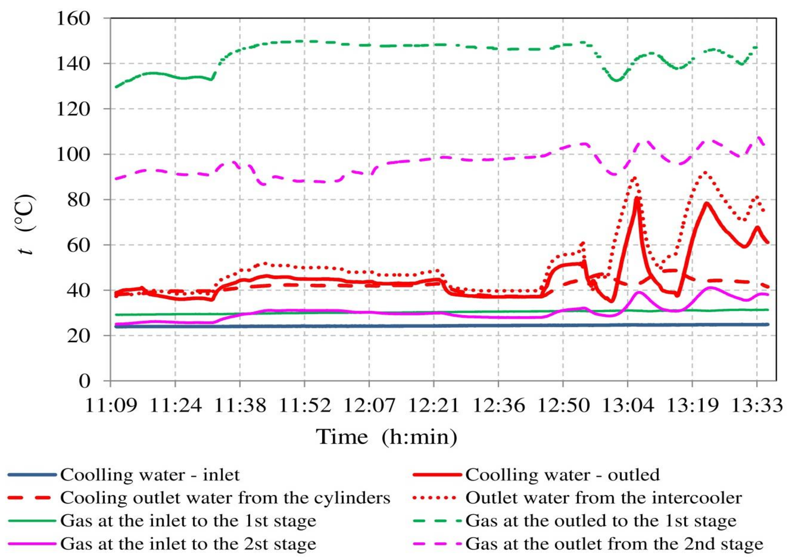
During the measurement, the atmospheric pressure did not change and its value was 99.9 kPa. Curves of all the water and gas temperatures are shown in
Figure 4. The temperature fluctuations in the terminal section of the graph are caused by adjusting the rate of flow into the intercooler and the terminal aftercooler using the regulating valves.
The measurement was carried out using the compressor running in a stable operation. When the operating parameters were changed, it was necessary to maintain and stabilise the gas and the cooling water temperatures within a period of 3 to 36 min (depending on the severity of the change in the operating parameters).
During the measurements, the operating conditions (inlet gas pressure, compressor revolutions, and cooling water flow rate) were deliberately changed to avoid the need for the long-term monitoring of individual compressor parameters. After the stabilisation of the changed operating conditions, the monitored parameters were found to be of almost constant values. Such a procedure facilitated the shortening of the time interval that was necessary for the system diagnostics. All of the data presented in
Figure 5 and in the following figures represent the average values of ten consecutive measurements with the 10 s increments.
The water flow rate (
QVw) and the values of differences in the pressures of the inlet water and heated water (Δ
p), recorded at selected times, are shown in
Figure 5. The increase in the pressure difference at the times 12:33 and 12:41 is caused by closing the water flow into the neighbouring compressors that were not running during the measurement, while the cooling water from the central cooling system was still flowing through them. This increase in the pressure difference was also reflected in an increased rate of the cooling water flow through the measured compressor. The pressure difference, as well as the total cooling water flow rate, is thus significantly dependent on the number of compressors connected to the cooling circuit, which can cause failures during the device operations.
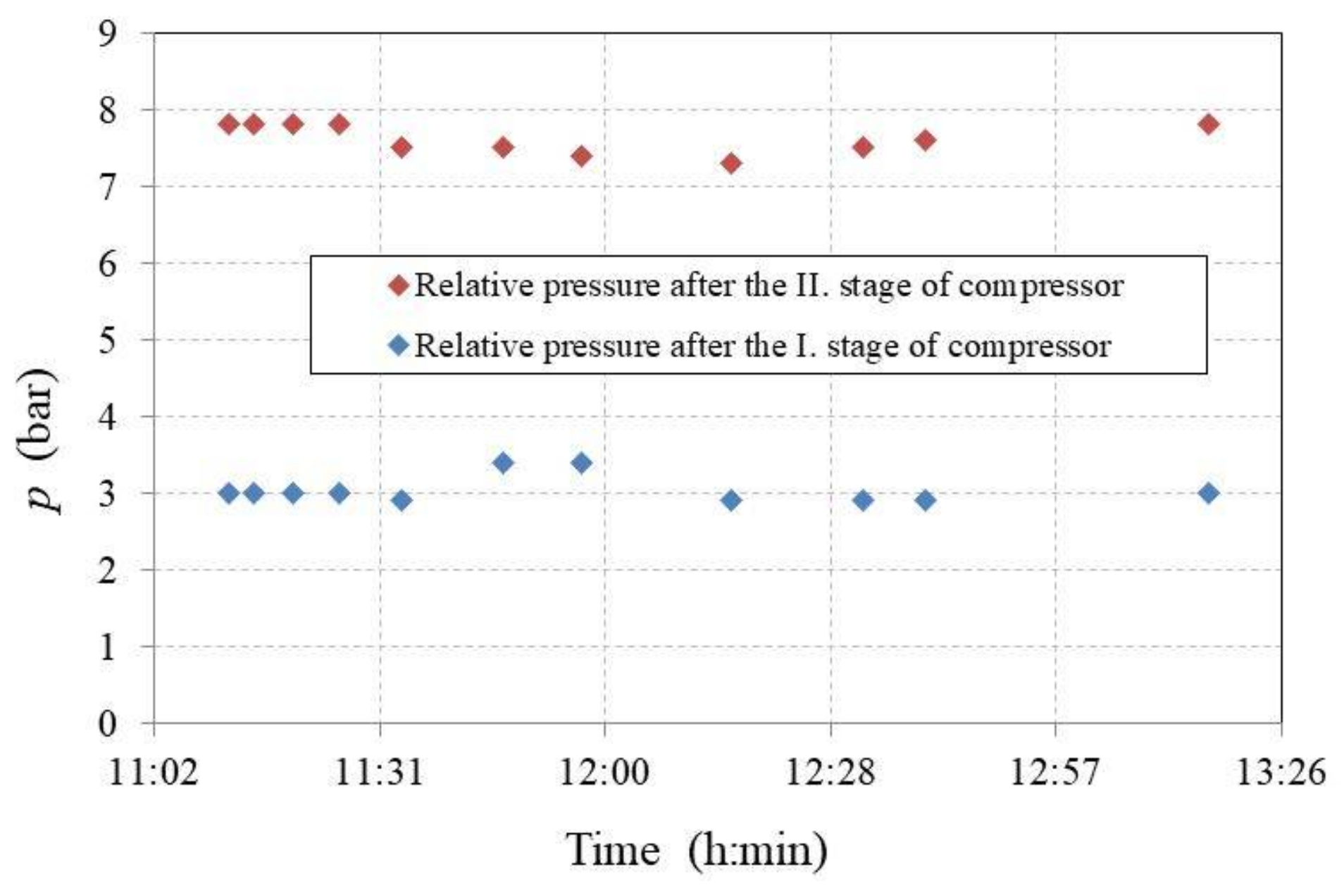
The measured relative gas pressure at the inlet to the compressor is shown in
Figure 6. At 1:47 and 11:57, it was raised to the maximum allowable value for the purpose of an analysis of its impact on the compressor’s operating parameters.
Figure 7 depicts the development of the relative pressure after the first and the second stages of the compressor.
Figure 8 represents the measured average electric current that was flowing through the first stage into the electric motor. A comparison of
Figure 6 and
Figure 8 clearly shows that the increase in the electric current becomes substantial mainly when the inlet gas pressure is elevated, which leads to an increase in the amount of compressed gas and thus also to an increase in the compression work.
The rated current for the used electric motor is 41 A, while the current protection device switches off the motor at a current of 43 A. This indicates that it is necessary to maintain the relative gas pressure at the inlet to the compressor at a maximum value of 10 kPa. The nominal relative output pressure is, according to the compressor technical data, 3 kPa.
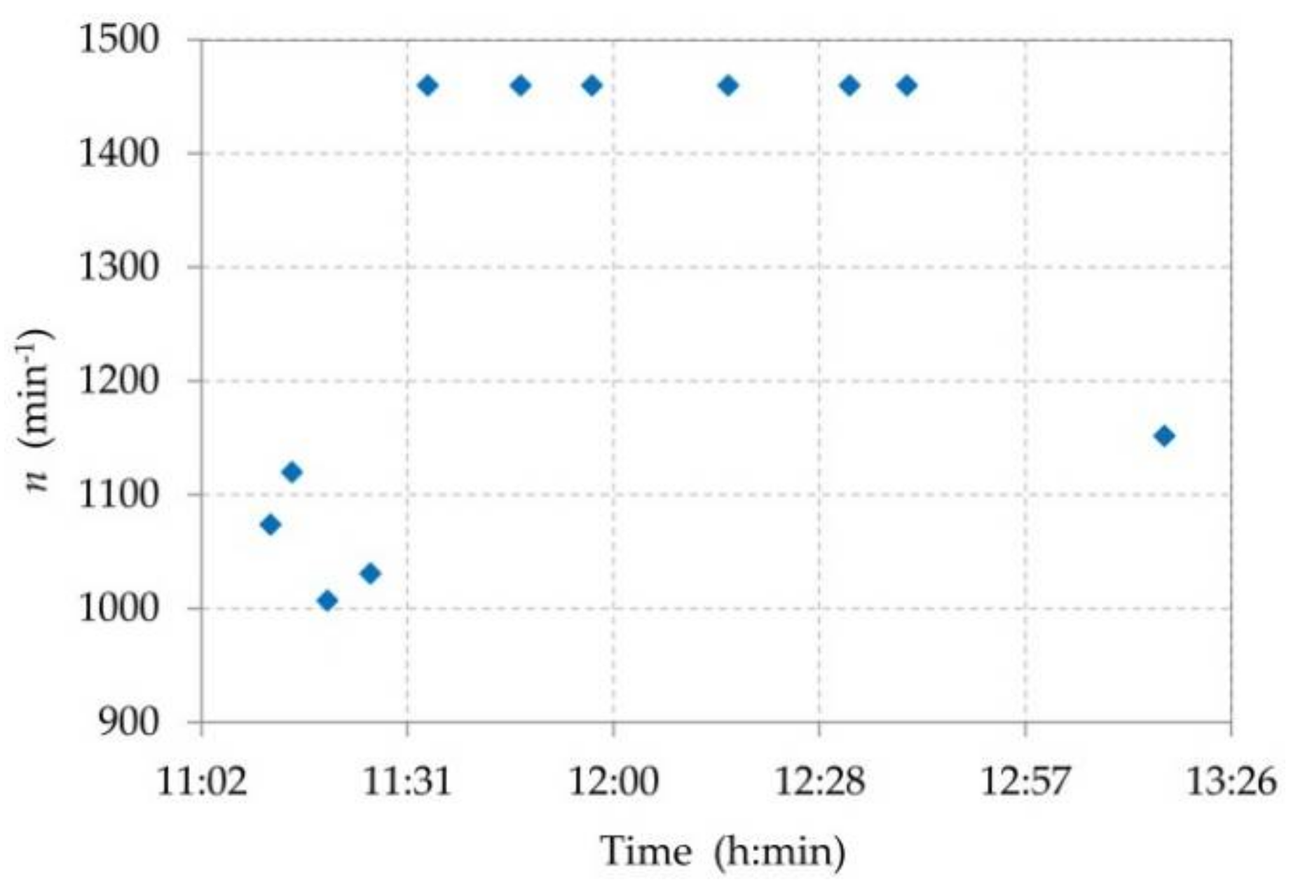
The motor rotation speed during the measured values ranged between the value of 1007 and the nominal value of 1460 min
−1 (
Figure 9). By increasing the revolutions up to the nominal value of 1460 min
−1, the electric current was increased. A correlation between the revolutions and the motor current cannot be identified, as the electric current depends on the mechanical power of the electric motor. A rapid increase of the input relative pressure (
Figure 6) changes the parameters of technical output, as defined by Formulas (5) and (6). Concurrently, there is a change in the thermal power due to the changing temperatures and flow rates of cooling water, affecting thus output parameters in Formula (1).
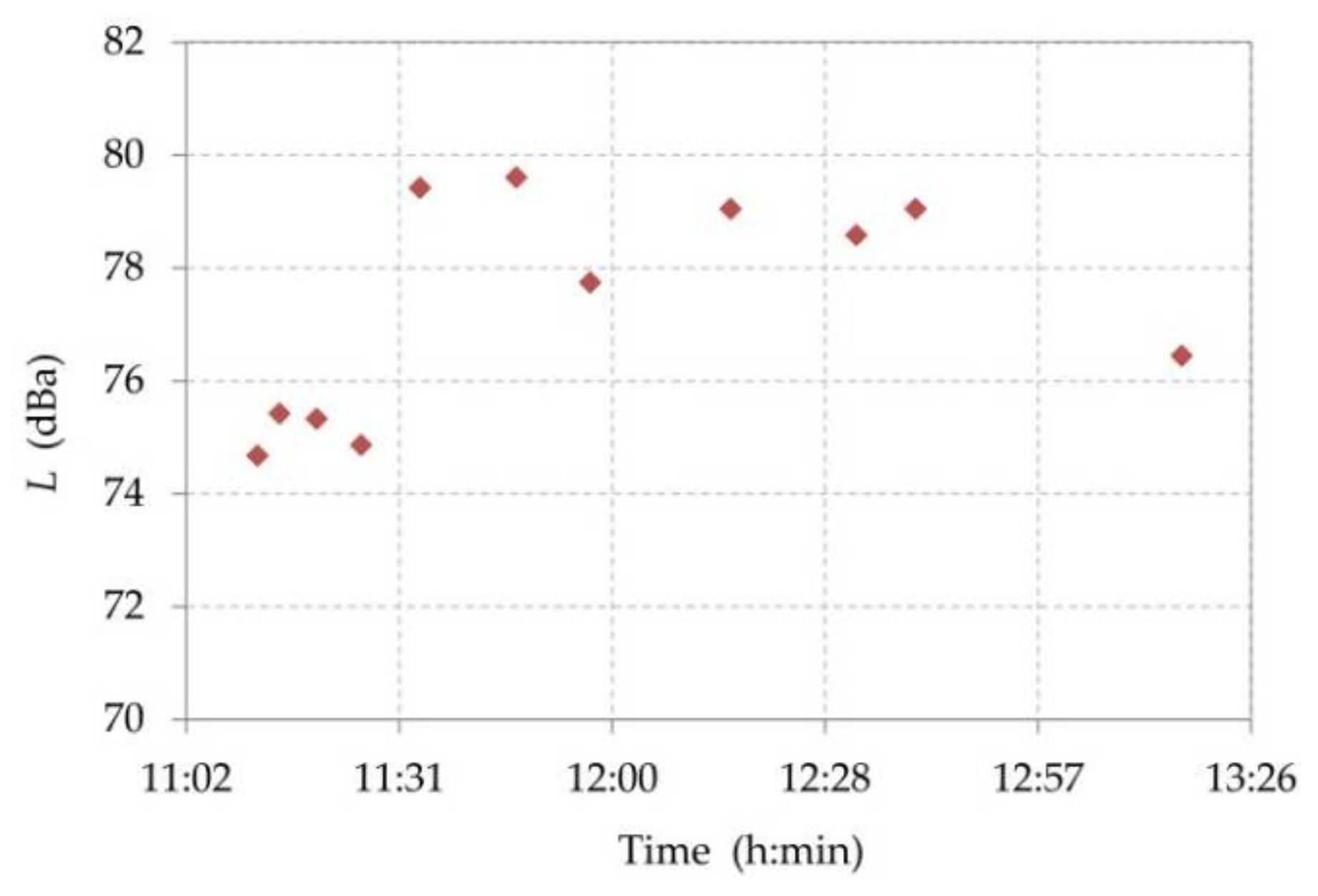
The measurement of the acoustic pressure level was carried out at the same conditions as stated in the compressor documentation (according to GAGI-PNEUROP): 1 m distance from the noise source; 1.5 m height from the floor. The measurement was carried out using the Norsonic 118 measuring device (measurement accuracy of ±2.1 dB
A, Gracey & Associates, Upper Dean, UK). The measurements were carried out at the same times as the measurements of the pressure, flow rate, and other parameters. They lasted 100 s with a sampling frequency of 8 Hz. Subsequently, the average acoustic pressure level
L was determined. The measurement results are listed in
Figure 10. The values do not exceed the maximum allowable level of acoustic pressure—80 dB
A. The highest values were reached when the electric motor was running at the nominal rotation speed.
3. Thermodynamic Analysis of the Compression of the Mixture of H2 and N2 Gases
To define potential causes of the Mehrer TZW 60/S6 compressor failures, it is necessary to determine the energy flows in the gas mixture compression process. On the basis of the energy balance, by calculating individual powers, it will be possible to determine the minimum required amount of cooling water. The power that is required to cover the technical work (
WT) will hereinafter be referred to as the technical power (
PTW). The energy balance of the compressor is based on the assumption that the total supplied mechanical power of the electric motor is split into the technical power of the polytropic compression in Stages 1 and 2 and the thermal power released during the compression, as described by the formula:
where
Pm is the mechanical power of the electric motor (W),
is the technical power of Stage 1 of the compressor (W),
is the technical power of Stage 2 of the compressor (W), and
Pts is the total thermal power of the compressor (including the heat loss) (W).
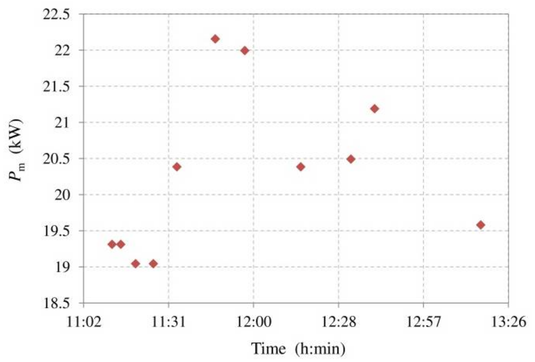
The mechanical power (
Figure 11) on the shaft, supplied into the compressor,
Pm, can be determined by using the formula:
where
I is the average electric current flowing through one coil of the electric motor (A),
Uz is the line voltage (400 V), cos
is the power factor (for the given electric motor it is 0.85), and
ηelm is the electric motor efficiency (1).
When the electric motor is connected in the Delta connection, then the current flowing through a single coil connected to the line voltage is as follows:
where
I1f is the measured value of the electric current flowing into the electric motor through a single phase (A).
The electric motor efficiency, calculated from the electric motor label data while using the Formula (4), is 91.1%:
where
Pmn is the nominal mechanical power on the shaft (W), and
In is the nominal electric current flowing through a single coil when the electric motor is in the Delta connection (A).
The technical power of the compressor Stages 1 and 2 is derived for the polytropic process of the compressor work [
14,
15]:
where
Qm is the mass flow rate of the mixture of H
2 and N
2 gases (kg·s
−1),
n1,
n2 are the polytropic exponents of Sages 1 and 2 of the compressor (1),
T1 is the gas temperature at the inlet into Stage 1 of the compressor (K),
T3 is the gas temperature at the inlet into Stage 2 of the compressor (K),
r is the specific gas constant of the mixture of the compressed gases (J·kg
−1·K
−1),
p1 is the absolute gas pressure at the inlet into Stage 1 of the compressor (Pa),
p2 is the absolute gas pressure at the outlet from Stage 1 of the compressor (Pa), and
p3 is the absolute gas pressure at the outlet from Stage 2 of the compressor (Pa).
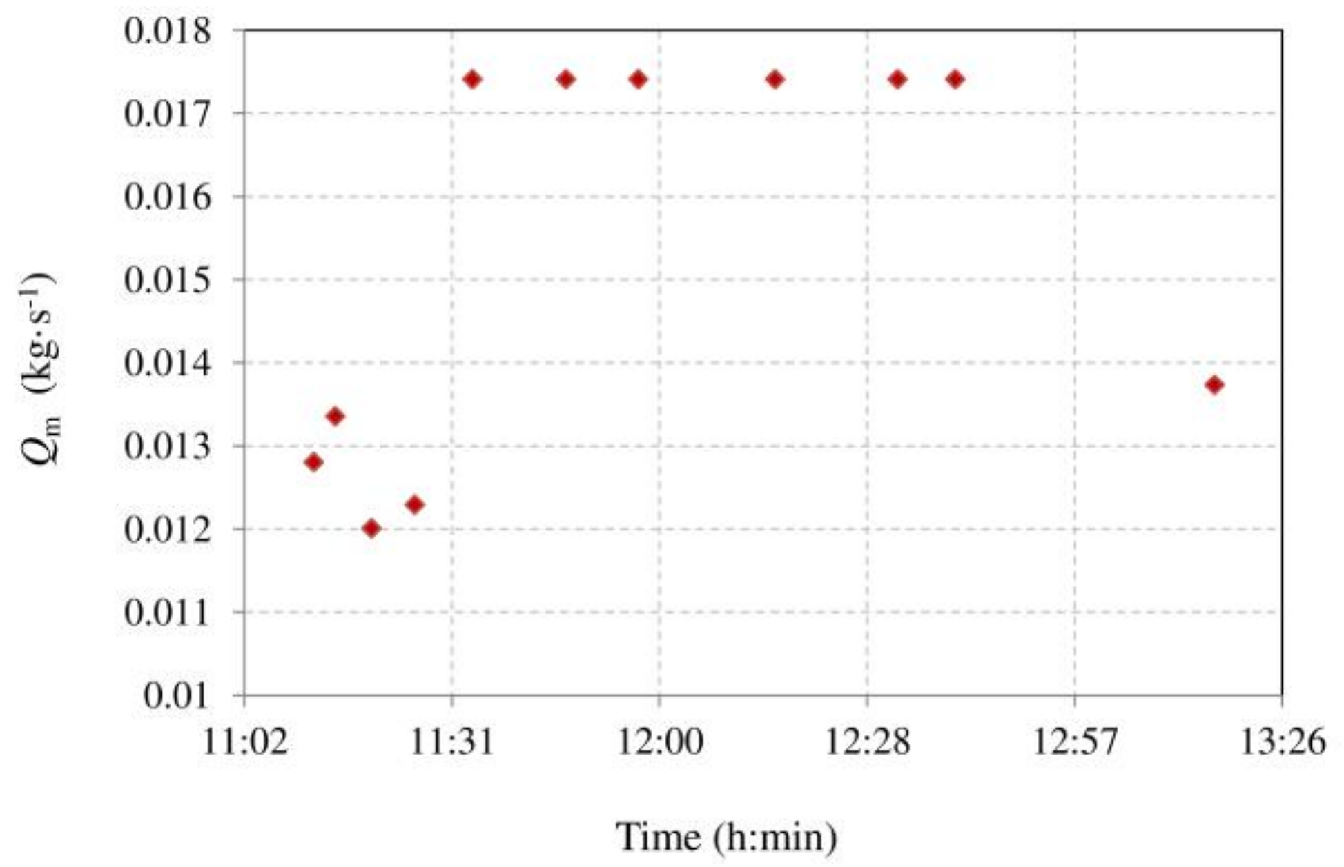
The mass flow rate of the gas is:
where
QV is the volumetric flow rate of the gas mixture at the inlet to the compressor (m
3·s
−1), and
ρ is the density of the gas mixture at the inlet to the compressor (kg·m
−3).
As the gas flow rate was not measured, its value was analytically obtained on the basis of the flow rate at the reference conditions (165 m
3·h
−1 at 0 °C and 101.325 kPa). The calculation of the volumetric flow rate of the gas at the inlet to Stage 1 of the compressor is derived, at the operational conditions, from the stated equation, while respecting the change in the compressor rotation speed. The compressibility factors of the gases are neglected when expressing the volumetric flow rate of the gas at the inlet to Stage 1 of the compressor, as they are approximately equal to 1 (at the pressure of 110 kPa and the temperature of 30 °C it applies that
zH2 = 1.00031,
zN2 = 0.99956). Then, the following applies:
where
Tn is the gas temperature at standard conditions (273.15 K),
pn is the pressure at standard conditions (101.325 kPa),
nc is the compressor rotation speed (min
−1),
ncn is the nominal rotation speed of the compressor (min
−1), and
QVn is the rate of the gas flow through the compressor at standard conditions (m
3·s
−1).
The gas mixture density was determined using the formula:
where
ri is the specific gas constant of the
ith component (J·kg
−1·K
−1), and
xi is the molar fraction of the
ith component of the mixture (1).
The calculated values of the mass flow rate of the gas that is flowing through the compressor are shown in
Figure 12.
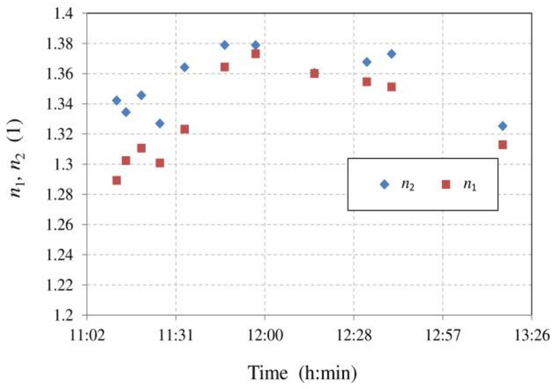
The calculations of the polytropic exponents
n1 and
n2 were based on formulas:
where
T2 is the gas temperature at the outlet from Stage 1 of the compressor (K), and
T4 is the gas temperature at the outlet from Stage 2 of the compressor (K). By a modification of Equations (10) and (11), we can obtain the formulas that are to be used for the calculation of the polytropic exponents of Stages 1 and 2 of the compression:
The values of the polytropic exponents
n1 and
n2 for Stages 1 and 2 of the compression are shown in
Figure 13.
4. Discussion on the Results
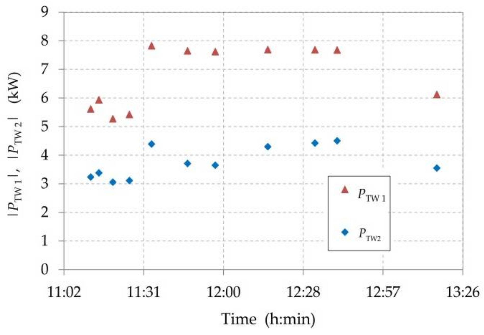
While applying the above described mathematical procedure, the technical powers were calculated and are listed for the measured parameters in
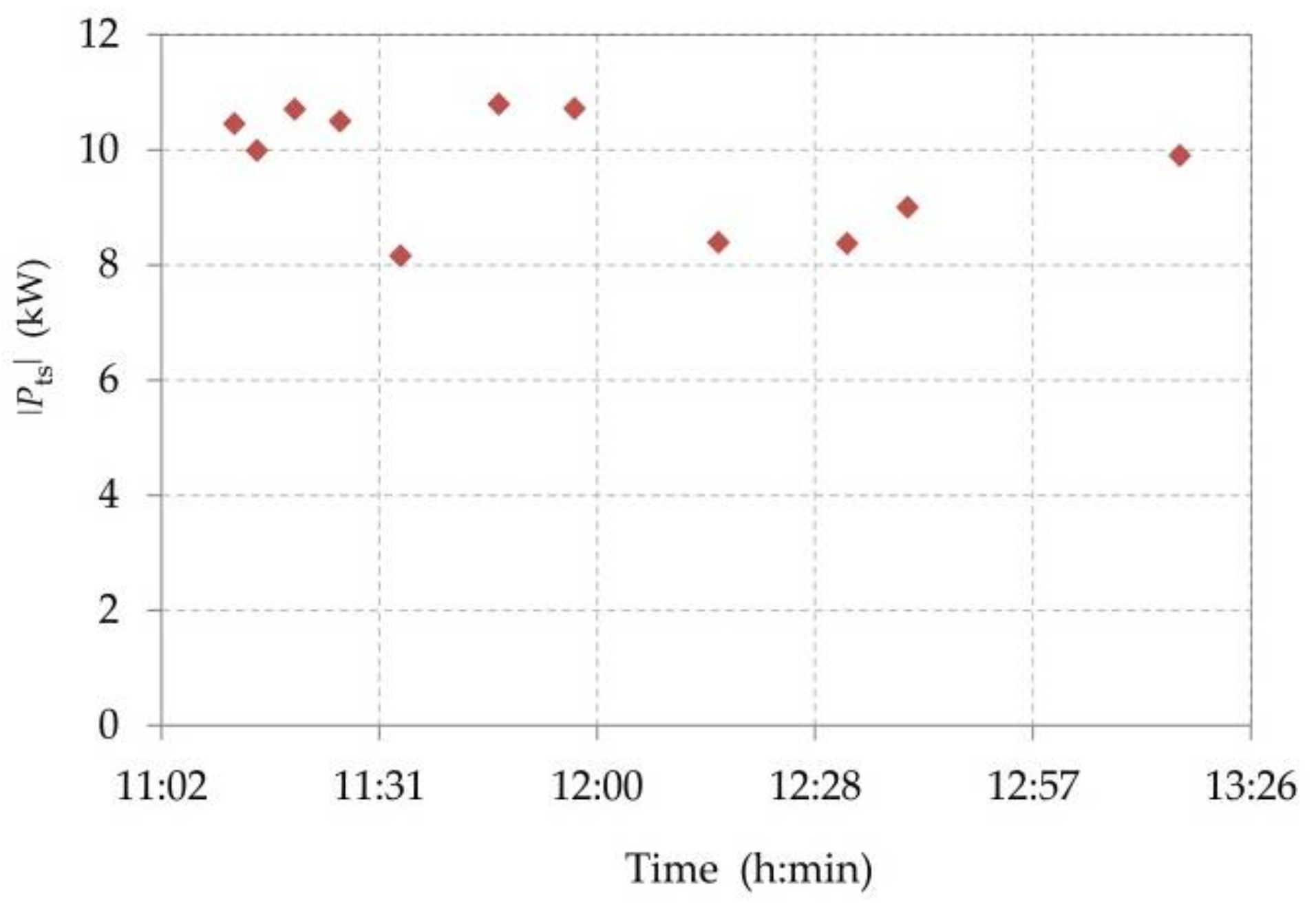
Figure 14. Once the mechanical power on the shaft and the technical power of the compressor are known, then the Formula (1) can be used to determine the total thermal power of the compressor
Pts (
Figure 15). During the gas compression, this power must be absorbed by the cooling water. The heat loss into the surrounding environment, which is caused by free convection and radiation, was identified by an approximate calculation of a maximum 2.4% of the total compressor input power and by considering the low level of, they were subsequently ignored.
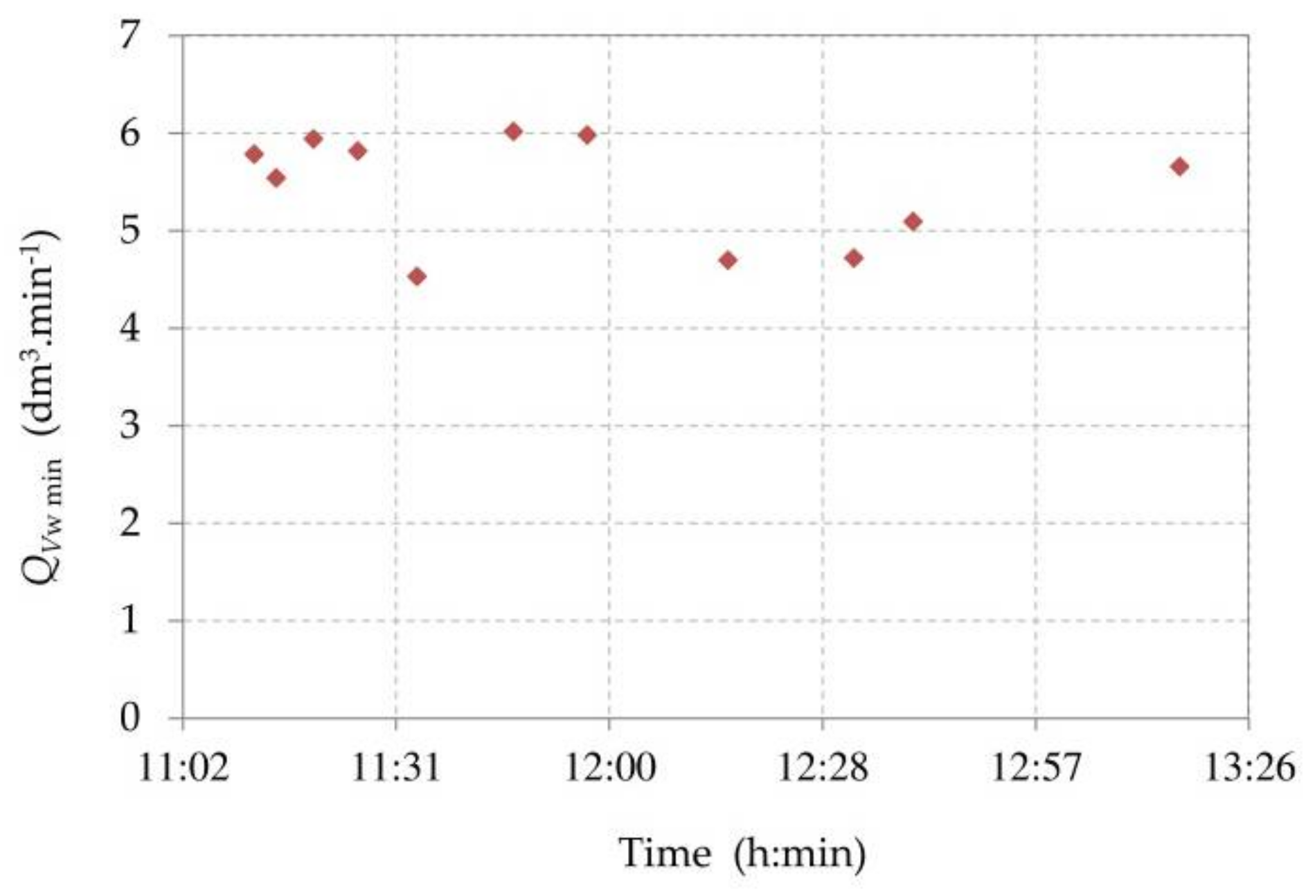
The minimum cooling water flow rate (
Figure 16) is determined using the Formula (14):
where
QVw min is the minimum cooling water flow rate (m
3·s
−1),
ρw is the water density at the mean temperature (kg·m
−3),
cw is the specific heat capacity of the water at the mean temperature (J·kg
−1·K
−1),
tw max is the maximum allowable temperature of the cooling water at the outlet from the compressor (°C), and
twi is the temperature of the cooling water at the inlet to the compressor (°C).
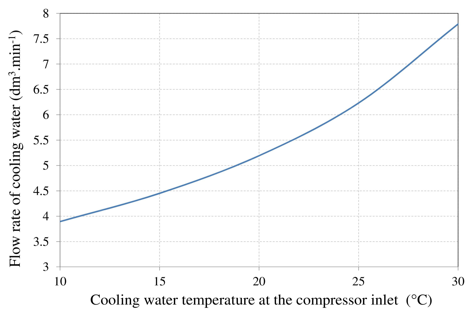
The minimum flow rate also depends on the temperature of the feed water. At the maximum compressor thermal power of 10.8 kW and at the maximum allowable outlet water temperature (50 °C), a sensitivity analysis of the minimum flow rate to the change in the cooling water inlet temperature can be carried out (
Figure 17).
The compressor was also tested at an outlet temperature of cooling water above 50 °C. This state corresponded to an increase in the electric current from the nominal value of 41 A to 43 A. The current increase was induced by the increase in the gas overpressure at the inlet to Stage 1 of the compressor up to 25 kPa, which was representing an approximately 2.5-fold increase of the overpressure that was occurring in a regular operation at the inlet to Stage 1.
4.1. Potential Undesired Compressor Failures
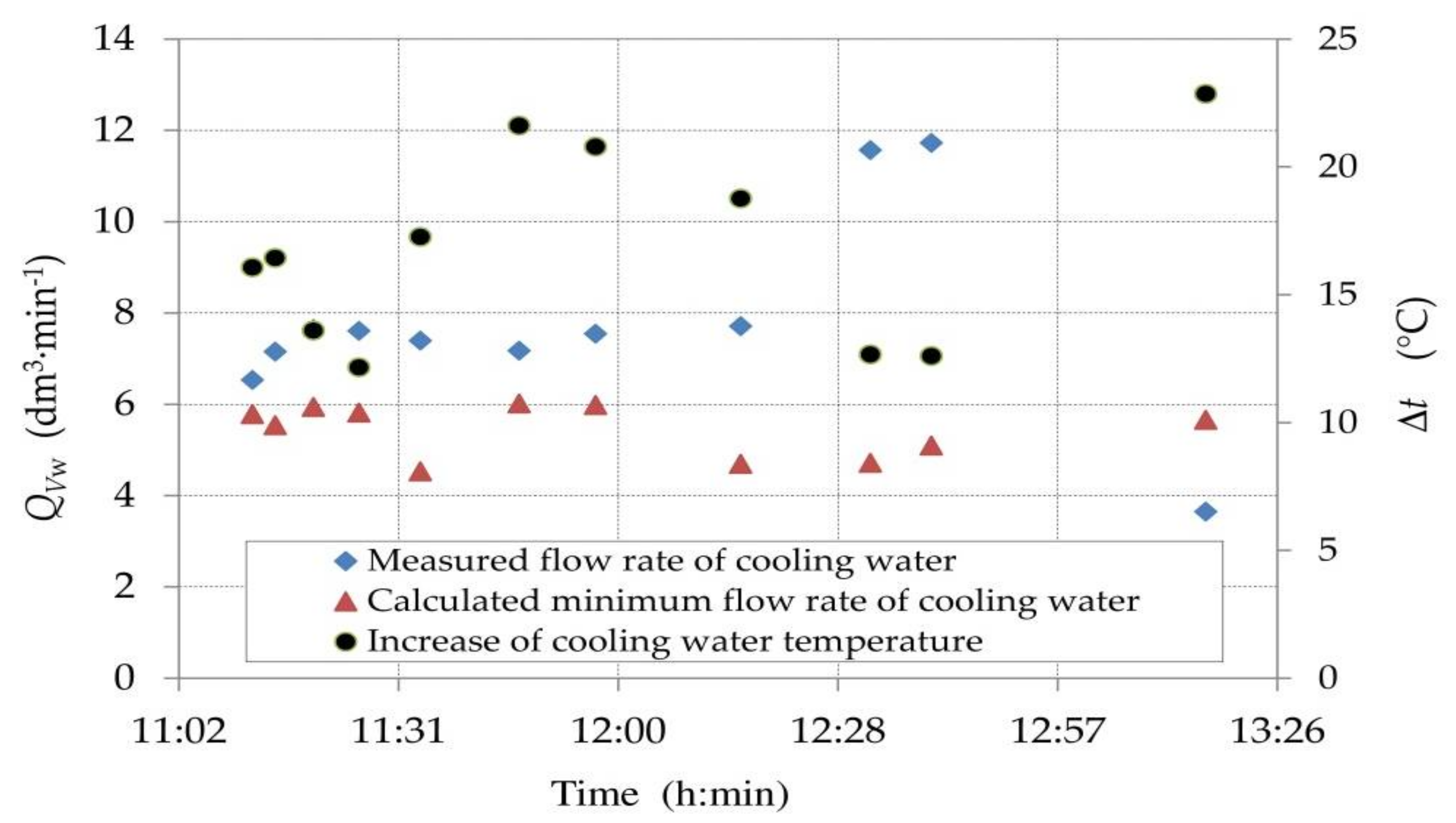
Measured and analytically determined cooling water flow rates, including the water temperature increase, are represented in
Figure 18. The comparison indicates that the measured flow rates are higher than the flow rates that were identified by calculations (except for the last measurement at 13:17). During this measurement, there was an unexpected closure of the regulating valve that resulted in a decrease in the pressure difference between the cooling water inlet and the water outlet. This reduced the rate of the cooling water flow into the intercooler. The flow rate decrease resulted in an increase in the cooling water temperature at the outlet from the aftercooler, as well as an increase in the temperature at the outlet from the cooling of the cylinders. If such a state lasted for a longer period of time, then it would result in an increase in the cooling water temperature at the outlet from the cylinders above 50 °C and in the emergency stop of the compressor.
The water flow rate can be approximately controlled by using its dependence on the pressure difference between the cooling water inlet and outlet, as described by the formula, determined by the regression analysis between the pressure difference and the measured flow rate, as shown in
Figure 5.
Such dependence is only applicable within the pressure difference range from 80 to 255 kPa. The pressure difference depends on the degree of presence of impurities in the water circuit; thus, the procedure that is described above is only approximate.
When the cooling water flow rate decreases, there is also an increase in the consumption of electric power input into the electric motor. An extreme case occurs when the cooling water supply is completely stopped. In such a case, the heat is no longer withdrawn and adiabatic gas compression occurs.
4.2. Compressor Status during Adiabatic Compression
When the cooling of the compressor cylinders is stopped after Stage 1, the gas pressure will be determined using the formula:
where
p2ad is the gas pressure after Stage 1 (Pa), and
κ is Poisson’s constant (for nitrogen and hydrogen
κ = 1.4) (1).
The temperature of the compressor after Stage 1 in the adiabatic compression is defined by the formula:
where
T2ad is the gas temperature after Stage 1 (K).
The pressure and temperature of the compressor after Stage 2 are determined analogically.
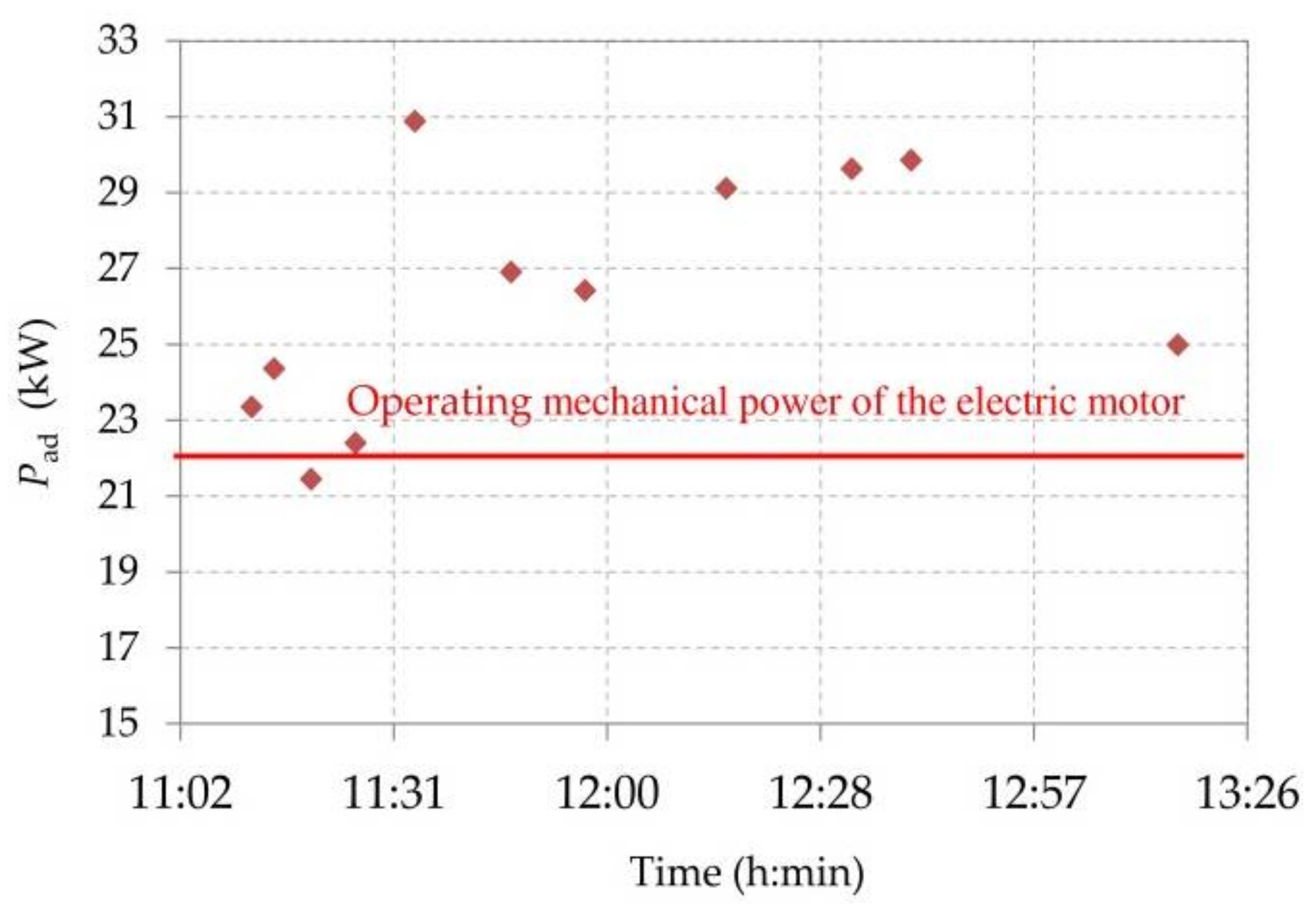
The calculated values of the mechanical power that are required during adiabatic compression are shown in
Figure 19.
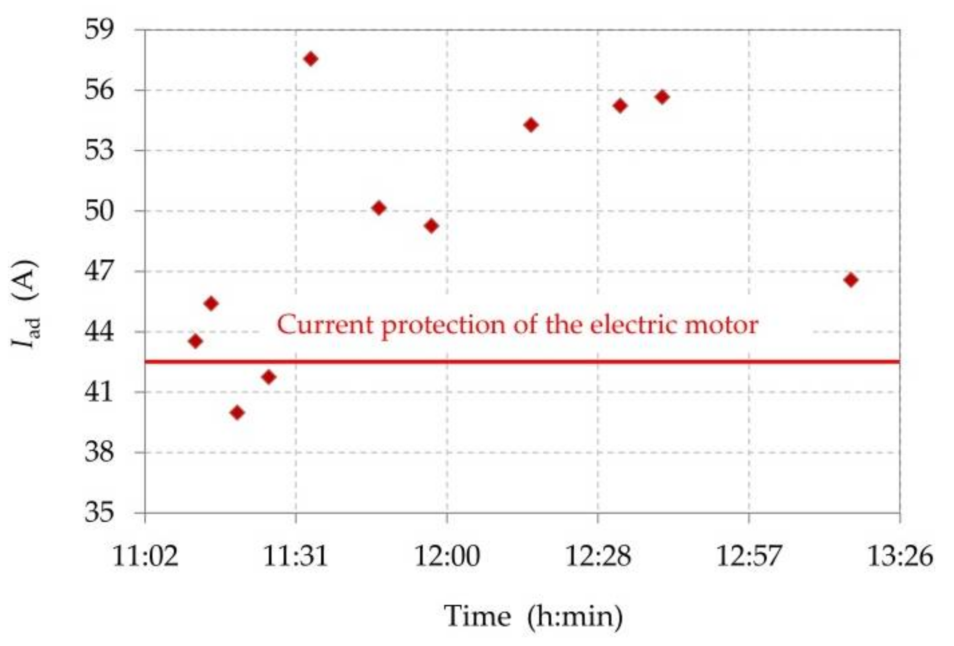
Using Formulas (2) and (3), it is possible to retroactively calculate what amount of the current (
Figure 20) would flow through Stage 1 into the electric motor, if the mechanical power on the shaft of the electric motor was as it is shown in
Figure 19.
Figure 20 indicates that, in the case of a compressor cooling failure, there would be a stoppage of the electric motor power supply at almost all of the measurement times, i.e., an electric motor failure would occur.
The adiabatic process is an extreme case of compression. It is apparent that, with decreasing rates of the cooling water flow, the required mechanic power of the electric motor shaft increases because the compressor approaches adiabatic compression. Therefore, to avoid a potential current protection switch-off, it is always necessary to ensure the determined minimum cooling water flow rate.
Another factor that may cause a compressor switch-off is an excessive increase in the outlet gas pressure. Higher pressure leads to an increase in the compression work, and also an increase in the current that is withdrawn by the electric motor.


