Study on Path Planning Method for Imitating the Lane-Changing Operation of Excellent Drivers


1
School of Automobile and Traffic Engineering, Jiangsu University, Zhenjiang 212013, China
2
Automotive Engineering Research Institute, Jiangsu University, Zhenjiang 212013, China
3
Electrical and Computer Engineering, Wayne State University, Detroit, MI 48202, USA
*
Author to whom correspondence should be addressed.
Appl. Sci. 2018, 8(5), 814; https://0-doi-org.brum.beds.ac.uk/10.3390/app8050814
Submission received: 22 April 2018
/
Revised: 11 May 2018
/
Accepted: 15 May 2018
/
Published: 18 May 2018
(This article belongs to the Special Issue Advanced Mobile Robotics)
Abstract
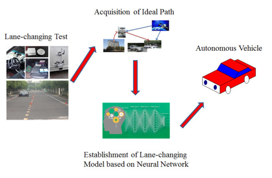
:Lane-changing is an important operation of an autonomous vehicle driving on the road. Safety and comfort are fully considered by excellent drivers in lane-changing operation. However, only the kinematic and dynamic constraints are taken into account in the traditional path planning methods, and the path generated by the traditional methods is very different from the actual trajectory of the vehicle driven by the excellent driver. In this paper, a path planning method for imitating the lane-changing operation of excellent drivers is proposed. Five experienced drivers are invited to do the lane-changing test, and the lane-changing trajectories data under different conditions are recorded. The excellent driver lane-changing model is established based on the genetic algorithm (GA) and back propagation (BP) neural network trained by the data of the lane-changing tests. The proposed approach can plan out an optimized lane change path according to the vehicle condition by learning the excellent drivers’ driving routes. The results of simulations verify that the path generated by the proposed algorithm is basically same as the track selected by the excellent drivers under same conditions, which can reflect the characteristics of the operations of the excellent driver. While applying safe lane-changing to autonomous vehicle, it can improve the ride comfort of the vehicle and therefore reduce the probability of motion sickness of the passengers caused by improper operation during lane change.
1. Introduction
In recent years, with the continuous increase in vehicle ownership, the problem of traffic safety has been deteriorating. Smart vehicles and unmanned driving that can effectively improve traffic safety are being vigorously developed and applied. Path planning that generates a driving route from the initial point to the destination is one of the keys features of unmanned driving technology. For autonomous vehicles, the constraints of vehicle kinematic and dynamics are important to be studied in path planning algorithm in addition to the obstacles avoidance.
Path planning methods for autonomous vehicles have been widely studied. There are some advanced path planning methods for autonomous road vehicles, such as artificial potential field methods [1,2] and optimal control [3,4]. The obstacles, road structures, and vehicle dynamics are considered in these proposed methods. However, there is a sudden change in the curvature of the trajectory generated by these methods, and it is often necessary to smooth the generated path and increase the workload. Many studies about curvature–continuous path planning methods have been conducted [5,6,7]. In these studies, some continuous curves such as Bezier curve are used for trajectory planning. Choi et al [7] proposed a practical path planning algorithm based on Bezier curves for autonomous vehicles operating under waypoints and corridor constraints. The path planning algorithm combines a set of low-degree of Bezier curve segments smoothly to generate the reference trajectory. However, since the planned path has difficulty meeting all comfort requirements of different passengers, it may still increase the probability of the motion sickness. Michael and Brandon [8] found that the proportion of people with motion sickness riding smart vehicles is much higher than traditional vehicles. Other studies have proven this conclusion [9,10]. As a result, conventional path panning algorithm is not sufficient to meet motion comfort requirements in these scenarios. However, under any condition, an experienced driver is always able to find an optimal path to keep the vehicle moving steadily. Thus, it is necessary to study the driving paths of experienced drivers.
Lane-changing is an important part of autonomous driving behavior in arterial road traffic [11], which involves changes in both longitudinal and lateral velocity as well as movement in the presence of other moving vehicles [12]. Therefore, many studies have been carried out on lane change of autonomous vehicle [13,14]. Dubins path, the shortest path for a wheel-drive robot consisting of a set of two circular arcs and line segments [15], is one of the most well-known and widely studied methods to generate a smooth path [16]. Chop et al [17] presented a path planning method using circle curve as the lane-changing path for autonomous vehicle. However, the path has a fatal drawback that the curvature at the joint nodes connecting the lines and arcs is discontinuous.Ren et al [18] presented a lane-changing trajectory generating method based on the vehicle lateral acceleration during lane changing meeting the constraints of positive and negative trapezoid. Wang et al. [19] used the seven-order polynomial as the path expression of the lane-changing path. The location of lane changing ends is determined according to the average lane changing time assuming that the longitudinal speed is constant. However, the characteristics of different drivers in the actual lane changing operation were not considered in these studies.
The artificial neural network is a powerful, nonlinear, and adaptive mathematical model [20]. It has been used extensively and successfully in various fields, including image processing [21], pattern recognition [22] and voice recognition [23]. It is difficult to describe the characteristics of the actual driver’s lane-changing operation by accurate mathematical modeling. Thus, the neural network is utilized to establish the lane-changing path model. In previous studies, by purposely propagating output-layer errors into hidden-layers, and deriving the optimal weights with gradient descent optimization [24], Back Propagation (BP) neural network is widely used to minimize errors. However, the further development and application of BP neural network is limited by the drawback that it easily falls into local optimal solutions. Many researchers have attempted to use different types of evolutionary algorithms, such as Genetic Algorithm [25], Particle Swarm Optimization (PSO) [26], and Simulated Annealing (SA) [27], to optimize the weight and threshold of the BP neural network in training process. Yu and Xu [28] presented a short-term load forecasting model of natural gas based on Genetic Algorithm and Back Propagation (GA-BP) neural network. Wang et al. [29] proposed a wind speed forecasting model based on GA-BP neural network. They found that the accuracy and the learning speed of the BP neural network can be improved significantly with optimization through the genetic algorithm.
To solve the problem that the traditional path planning methods for lane-changing do not consider the actual driving characteristic of lane-changing, five excellent drivers were invited to do lane-changing tests. The trajectories under different modes were recorded. The paths were fitted by polynomial curve by comparing different curves. The routes of lane-changing considering the feature of the intermediate state and the final position were obtained. The excellent driver lane-changing model was established based on GA-BP neural networks trained by the optimal trajectory database obtained by the experiment. The path planning method for lane-changing based on the excellent driver lane-changing model was proposed. It can meet the requirements of different types of passengers for riding comfort and reduce the probability of motion sickness.
The structure of the paper is as follows. Section 2 presents the lane-changing test, and gives an approach to transform the data of Global Position System (GPS) into geographic coordinate system. The fitting of driver’s lane-changing path based on six-order polynomial is shown in Section 3. In Section 4, the excellent driver model based on GA-BP neural networks is highlighted. Simulation results are discussed in Section 5. Finally, Section 6 presents some concluding remarks.
2. Acquisition of Ideal Path
2.1. Lane-Changing Test
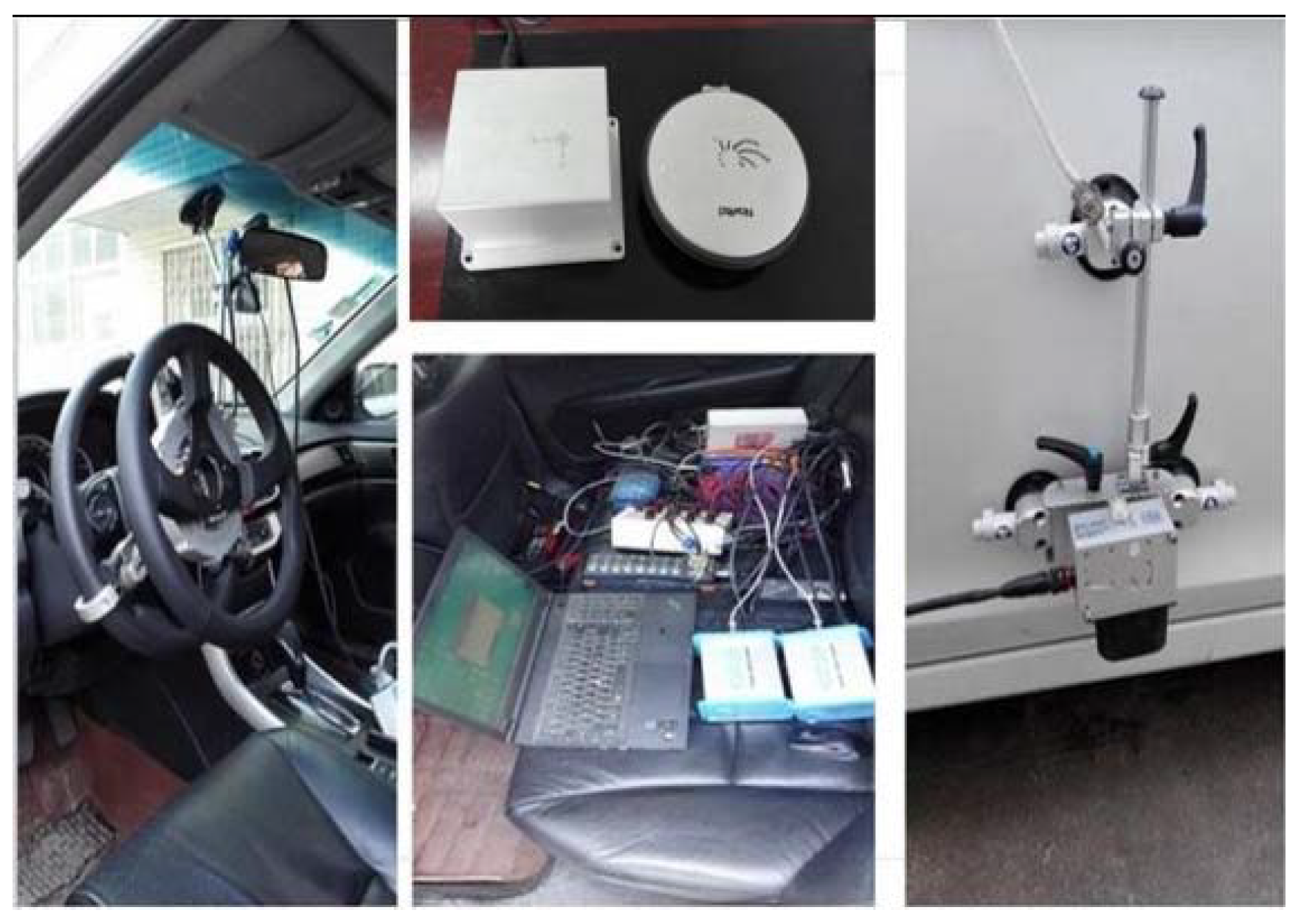
Lane changing is one of the important operations in driving. The driver will plan out an ideal path to make the vehicle move smoothly before starting to change lane. To study the characteristics of the path that the excellent driver planned at the time of lane changing, driving tests with excellent drivers were carried out. Figure 1 shows the test vehicle used in this experiment. It is equipped with GPS device to record the travel path and S-Motion biaxial optical speed sensor to obtain the yaw rate and lateral acceleration of the vehicle. Due to the difference of driving experience and driving habits, different drivers usually have different driving characteristics. An evaluation questionnaire about the types of driver was designed. After each experiment, the passenger appraised the ride experience. Thus, the drivers were divided into three types based on the driving characteristics: aggressive, intermediate and conservative. To track the difference in lane-changing paths between different drivers, five experienced drivers were invited to participate in the experiment. Information of the five drivers is shown in Table 1. During driving, the drivers were required to do the lane-changing operation to meet the demand of obstacle avoidance or overtaking as well as others operation. In this experiment, the test was divided into two working conditions: obstacle avoidance lane change and free lane change. The single lane change test was conducted as the obstacle avoidance condition by changing the pile position to simulate different obstacle distance. Figure 2 shows the single lane change test environment.
2.2. Data Processing
Owing to the data recoded by GPS being longitude, latitude and elevation, it is difficult to directly reflect the vehicle’s actual running path in the geodetic coordinate system. In geographic coordinate system, the origin of the coordinates lies in the centroid of the carrier, and its Xg axis, Yg axis and Zg axis are the east, north and sky directions, respectively, of the carrier’s location. To accurately describe the travel path, it is necessary to transform the coordinates of the geodetic coordinate system into the geographic coordinate system. However, a direct conversion of coordinates between the geodetic coordinate system and the geographic coordinate system is hard to process. Therefore, the Earth Cartesian coordinate system is introduced into the transformation. The relationships between the geodetic coordinate system, the geographic coordinate system and the Earth Cartesian coordinate system are shown in Figure 3.
The coordinates of the point P is (L, λ, h) in geodetic coordinate system. The coordinates of the point P (xe, ye, ze) in the Cartesian coordinate system can be obtained from Equation (1).
where RN is the radius of curvature of the ellipsoid, RN = Re(1 + esin2L). e is eccentricity of ellipsoid, e = (Re − Rp)/Re. Re is the long radius of the ellipse and Rp is the short radius of the ellipsoid.
The travel path of the vehicle is a spatial curve connected by many spatial points in geodetic coordinate system. The spatial curve needs to be projected to the xg − yg plane in the geographic coordinate system. To facilitate the analysis of the driving path, the coordinate origin of the geographical coordinate system is set at the initial record point of the driving track. Thus, the coordinates of each sampling point in the Earth Cartesian coordinate system needs to be transformed by Equation (2).
Then, the coordinates of the Earth Cartesian coordinate system are transformed into the coordinates of the geographic coordinate system using Equation (3).
With the above transformations, the driving path can be shown accurately in two-dimensional plane of the geographic coordinate system using the coordinate (xg, yg).
3. Fitting of the Test Path
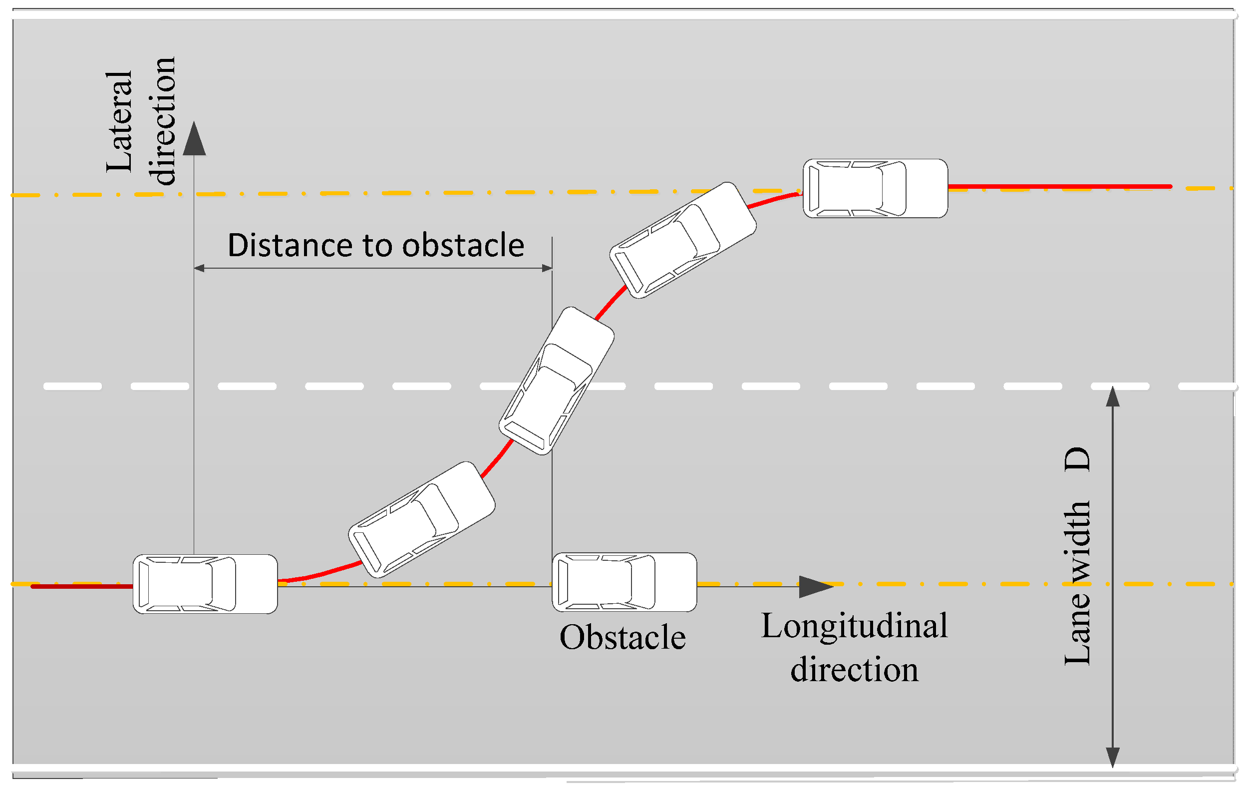
Function fitting refers to search a curve expression by adjusting some undetermined coefficients in this function to minimize the difference between the function and the known set of coordinate points (xi, yi). According to above process, the coordinates of the ideal path in the geographical coordinate system have been obtained. For the convenience of calculation, only the two-dimensional coordinate (xg, yg) is needed to be fitted without considering the vertical motion. Figure 4 is a schematic diagram of the lane-changing path.
It is necessary to satisfy the requirement of curvature continuity of the path curve to ensure the vehicle moves smoothly. Once the shape of the curve is known, the curvature–continuous fitting function should be determined. An easement curve is a curve of continuous curvature, usually set between a straight line and a circular curve or between two circular curves with different radius. There will be no mutation of the curvature of the path curve. Therefore, it can improve the comfort and stability of the vehicle considerably. There are usually two types of transition curves: clothoid and cubic parabola. In engineering practice, the swirl curve is obtained by the method of point selection and lofting. However, it is difficult to accurately fit the swirl curve, as its mathematical equation is too complicated, which will lead to high computation cost. The expression of polynomial curve is succinct, and all derivatives are continuous. It can accurately fit the driving path under different operation conditions by changing the coefficients of each item. In this paper, the polynomial curve is adopted as the lane-changing path.
Polynomial equations are set as follows:
where y′ is the first derivative and y″ is the second derivative of the polynomial curve. k is the curvature of a point on the curve.
The center of the mass of vehicle at the beginning of lane-changing is set as the origin of the coordinate system for simplifying the system with proposer assumptions. Thus, the polynomial constant term is zero. According to the analysis of lane changing operation, it is known that, at the initial and final state of the lane-changing operation, the vehicle’s heading direction should be parallel to the lane line and the steering angle shall be zero. To make the unmanned vehicle able to travel straight along the lane, it is required that the steering wheel angular speed be zero when the lane-changing operation ends. Therefore, the first derivative and the second derivative of the polynomial curve at the initial point and the final point are zero. The final point of lane-changing is set as (xf, yf) and yf is the lane width of the current driving road. Thus, the position of the vehicle is at the middle of the lane when lane-changing is completed. While the initial and final positions of lane-changing are determined, the trajectory selected by different types of drivers will also be different, which has impact on the riding comfort of the lane-changing process. Therefore, it is necessary to consider the intermediate state of the vehicle during lane-changing path planning. It is noticed that the entire lane-changing process can be divided into three phases: collision avoidance, rotation and adjustment [30]. It can be seen that the steering wheel angular speed during the obstacle avoidance and the rotation phase are faster than that during the adjustment phase by analyzing the steering wheel angular speed during the lane-changing process. Therefore, the vehicle position state (xm, ym) at the end of the rotation phase is adopted as the intermediate state constraint of the lane-changing operation. By substituting the state constraint of the initial point, final point and intermediate point into Equation (4), Equation (6) can be obtained as follows:
Substituting x0 = y0 = 0 and yf = D into Equation (6), Equation (7) is as follows:
From Equation (7), it is known that the number of polynomial coefficients need to be determined is n − 2, and the number of constraint equation is only4. To determine the unique expression of the lane-changing path, the equation (8) needs to be satisfied.
Thus, n = 6. The expression of the lane-changing trajectory is as follows:
The expression of the optimal lane-changing path under different conditions can be obtained with the middle point coordinates and the final distance of lane-changing determined.
4. Path Planning Method Based on Excellent Driver Lane-Changing Model
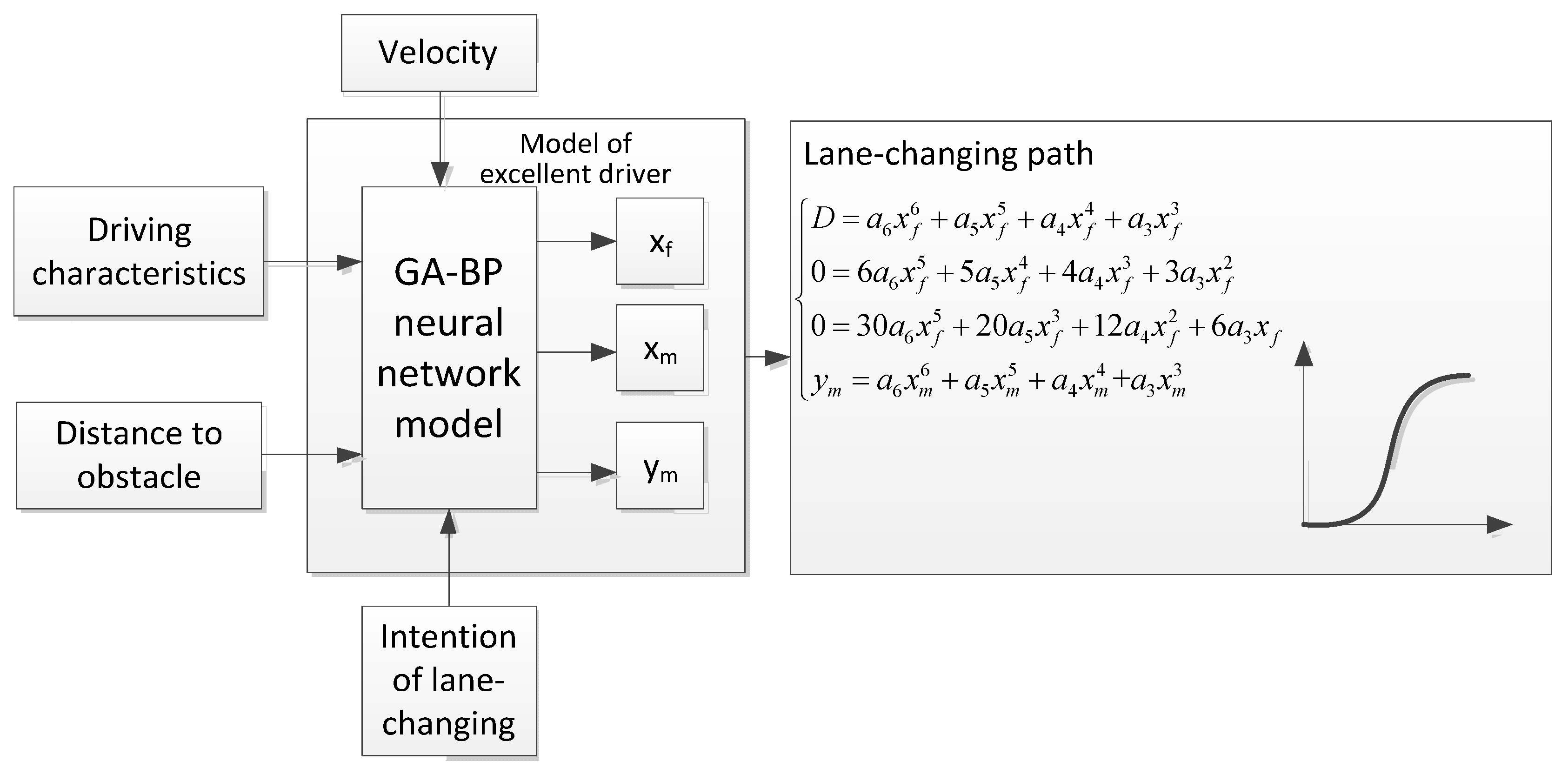
Lane-changing is an important and complex operation in vehicle driving. Trajectory has great influence on the comfort of the driverless vehicle. Optimal lane-changing trajectories of several excellent drivers under different conditions were obtained from previous research. The lane-changing model of excellent driver was established based on the GA-BP neural network trained and tested by the testing path data. The path planning method for imitating the lane-changing operation of excellent drivers is proposed. It can generate an optimal lane-changing trajectory according to the driving conditions of vehicles and the types selected by the passengers therefore improve the comfort of the autonomous vehicles. Figure 5 shows the framework of the path planning method for imitating the lane-changing operation of excellent drivers.
4.1. GA-BP Neural Networks
BP neural network is a multi-unit feed forward neural network, which can be trained by error back propagation. The error of the actual output value and the desired output value of the network is minimized by adjusting the weights and thresholds based on the gradient descent method. There are three units in the BP neural network: input layers, output layers and hidden layers. In the training process, there are two stages of forward and back propagation. In the stage of forward propagation, the input information is transmitted from the input layer through the hidden layer to the output layer. The state of each layer only affects the next layer state of neurons. The back propagation is introduced in the case the error is larger than the threshold. The weights of each layer of neurons are modified to minimize the error.
Genetic algorithm is a global optimization random search algorithm. It can get the individual with high adaptation degree by simulating the phenomena of selection, crossover and mutation in the genetic process. To solve the problem that BP neural network algorithm is easy to fall into local optimal solutions, the GA is used to optimize the initial weights and thresholds of BP neural network. The population of GA is generated based on the weights and thresholds of BP neural network. With going through the selection, crossover and mutation process, the optimal individuals are selected as the initial weights and thresholds of BP neural network. With GA, the convergence speed of the BP neural network can be improved significantly and the possibility of falling into local optimal solutions can be reduced. Figure 6 shows the GA-BP neural network algorithm flow chart. The specific algorithm is as follows:
(1) Initialization of the population
The initial population of scale P, X = (X1, X2, …, Xp)T, is randomly generated. The individual code, Xi = (x1, x2, …, xs), utilizes the real number coding method. The length coding is as follows:
where m is hidden layer nodes, n is input layer nodes and l is output layer nodes.
(2) Determination of the fitness function
In the GA-BP model, the use of a fitness function F is based on the error of the output layer. The function F is defined as:
where yj is the expected output. oj is the actual output based on the weights and thresholds generated in Step 1. k is compensation factor.
(3) Selection operation
This paper uses the roulette method to select the operator. The probability of each individual is calculated as follows
(4) Crossover operation
The crossover operation between the chromosome k and the chromosome l in the gene j is as follows
where b is a random number in [0, 1].
(5) Mutation operation
The mutation operation of the chromosome i in the gene j is as follows
where xmin and xmax are the minimum and maximum values of the xij, respectively. r is a random number in [0, 1]. r2 is a random number. g represents the current number of iterations and Gmax is the maximum number of evolutions.
4.2. Excellent Driver Lane-Changing Model
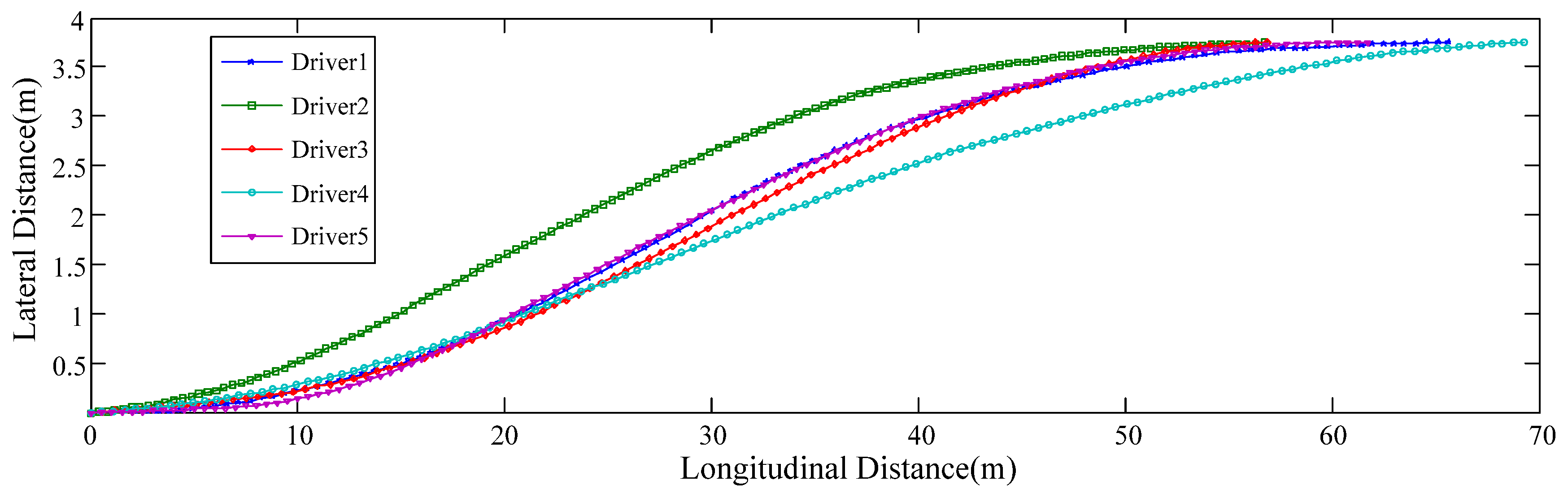
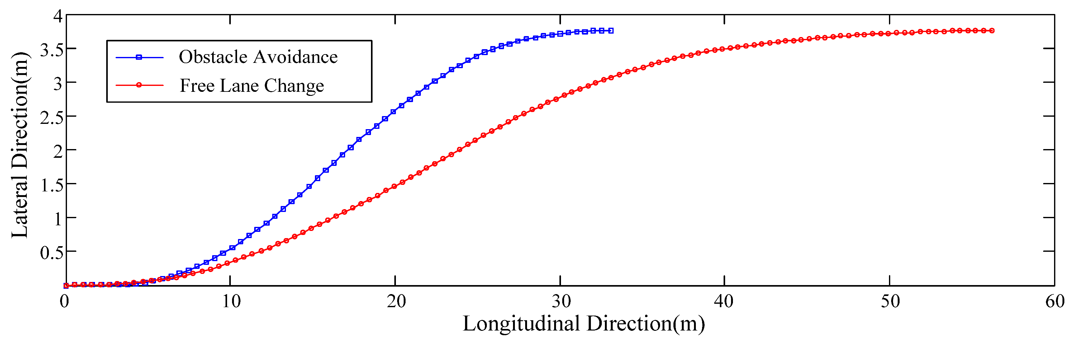
The lane-changing trajectories chosen by different drivers under the same working conditions will be different due to the various driving habits and personalities of each driver. Figure 7 shows the lane-changing paths of different drivers at the same speed. It can be observed that the driving characteristic is one of the most important factors that influence the travel route. Through the analysis of the operating habits of different drivers, the driver types are divided into aggressive, intermediate and conservative. In this research, 1 represents aggressive type, 0 represents conservative type, and 0.5 means intermediate type. Figure 8 shows the paths of the free lane change and the obstacle avoidance lane change. In the figure, it is shown that different steering intentions also create a considerable impact on the vehicle driving path. In this paper, 1 represents the intention of obstacle avoidance lane change and 0 is for free lane change. In addition, the speed and the distance from obstacle also have an impact on the choice of the lane-changing path. Figure 9 shown the lane-changing paths of one driver at different speeds. Therefore, the excellent driver lane-changing model in this paper has four inputs, namely driver type, steering intention, vehicle speed and distance from obstacle. According to the above analysis, the optimal lane-changing path under different conditions can be obtained when the characteristic point coordinates (xm, ym) and the final distance xf of lane-changing are determined. Thus, the model proposed in the paper has three outputs: xm, ym, and xf.
The experimental data are shown in Table 2. The steering intention is determined based on distance from obstacle. The distance from obstacle under free lane change condition is set to 100 m. Therefore, there are 300 experimental data. Ninety percent of the data were selected at random as the training data, while the remaining are the testing data.
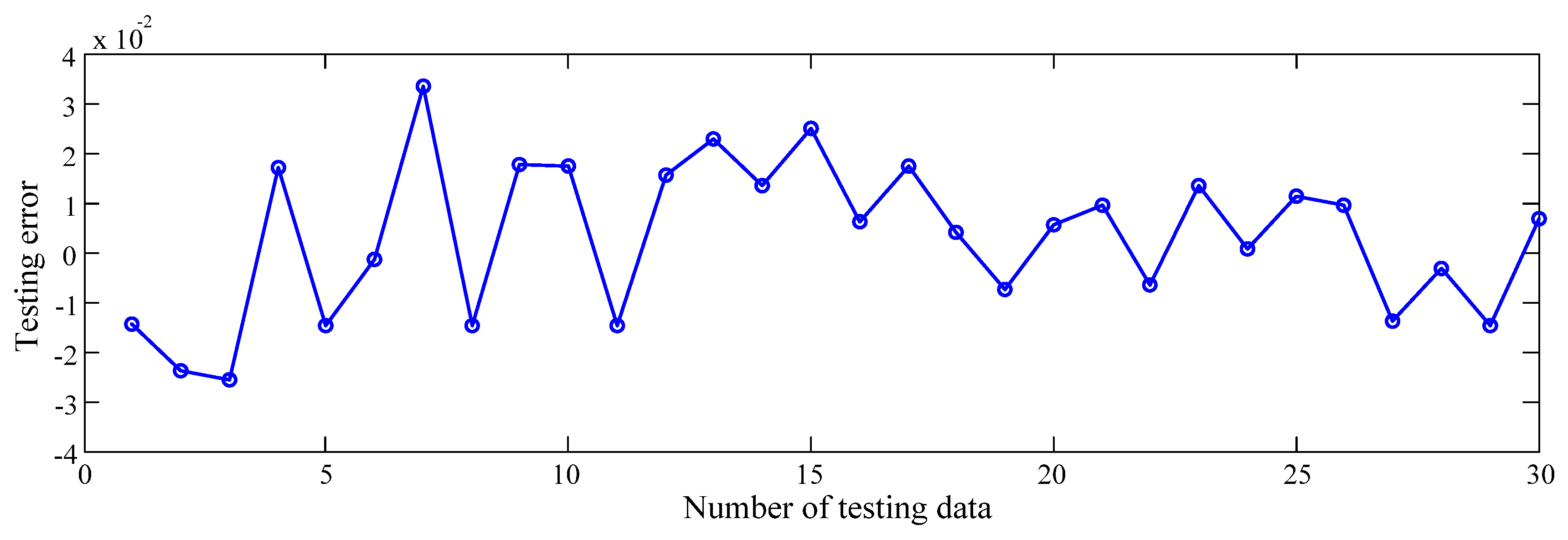
The effectiveness of the neutral network was estimated using the GA-BP error. The error is defined as the difference between the simulation output and experimental output as Equation (17). For the testing in this research, the error is shown in Figure 10. In the figure, it can be observed that the GA-BP neural network is with high accuracy.
where output_simu is the output value of the GA-BP neural network and output_testing is the value of the testing date.
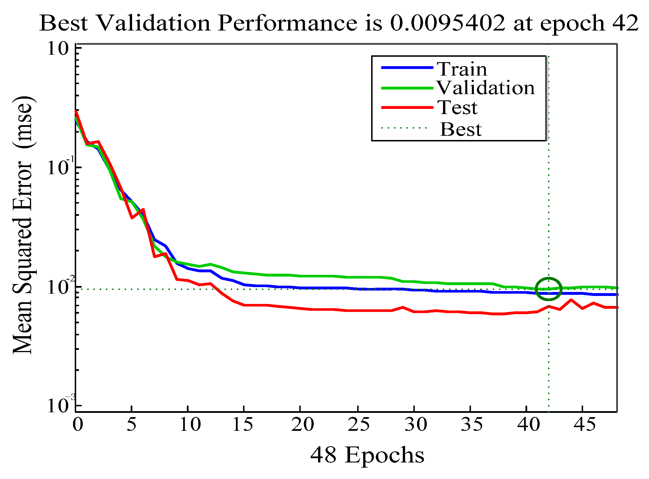
Figure 11 shows the mean square error variation curve of the GA-BP neural networks model. The mean square error is 0.009 after training, and it can meet the precision requirements.
5. Simulation and Analysis
To study the performance of the path planning algorithm based on the excellent driver model proposed in the paper, simulation experiments under different working conditions were carried out in MATLAB environments. The scenarios of obstacle avoidance steering and free lane-changing steering at the speed of 30 km/h and 40 km/h were simulated. In each simulation test, the aggressive and conservative types were selected as driver type, respectively. Then, the lane-changing trajectory generated by the proposed method was compared with the actual driving trajectory under the same working condition. The effectiveness of the proposed algorithm can be quantitatively evaluated by calculating the deviation between the actual value and the simulation value. The change of the error is also presented.
5.1. Obstacle Avoidance Simulation
Obstacle avoidance simulation test conditions: The speed is set to 30 km/h and 40 km/h, respectively; lane width is 3.75 m; and the distance to obstacle at the beginning of steering is 35 m.
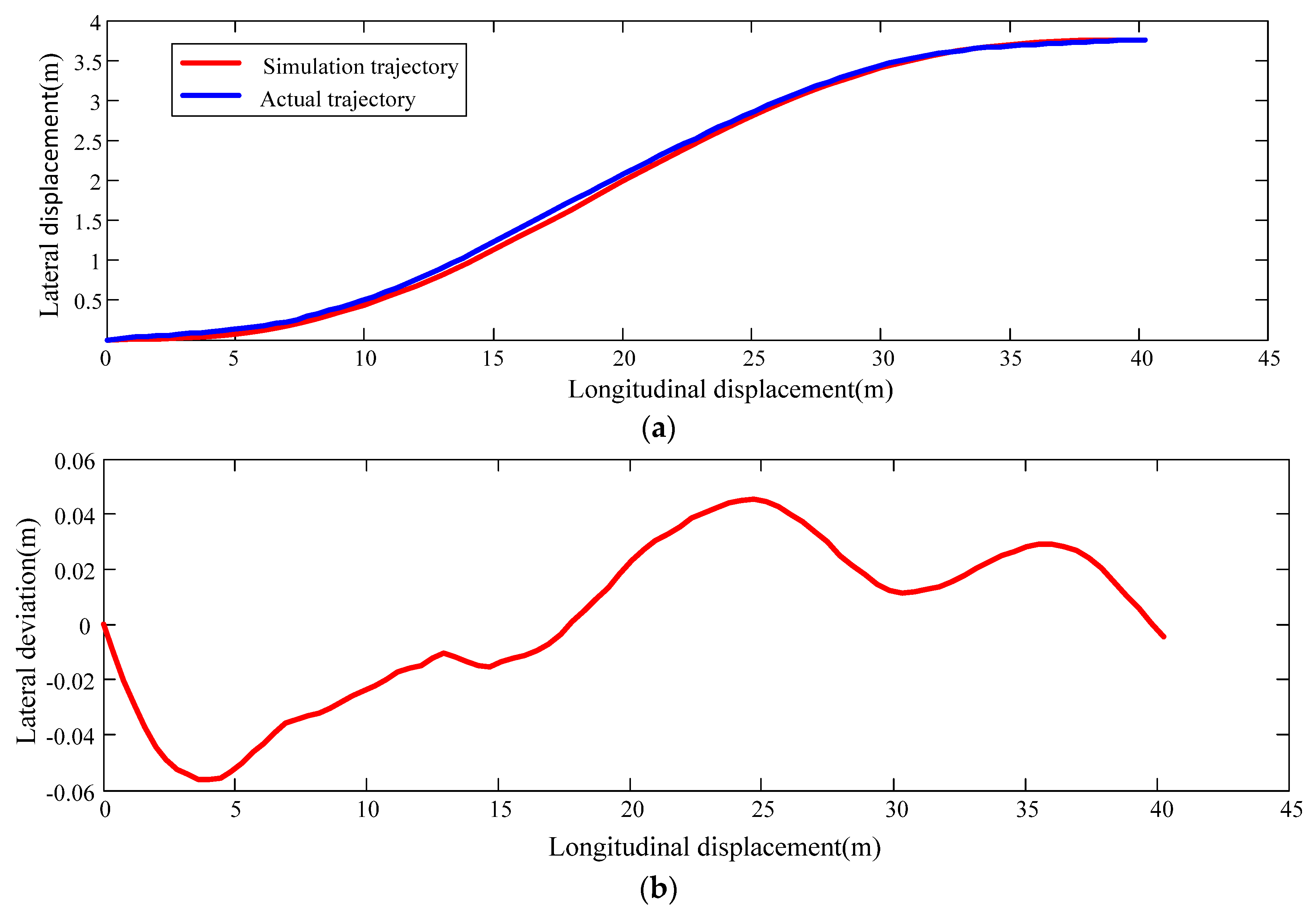
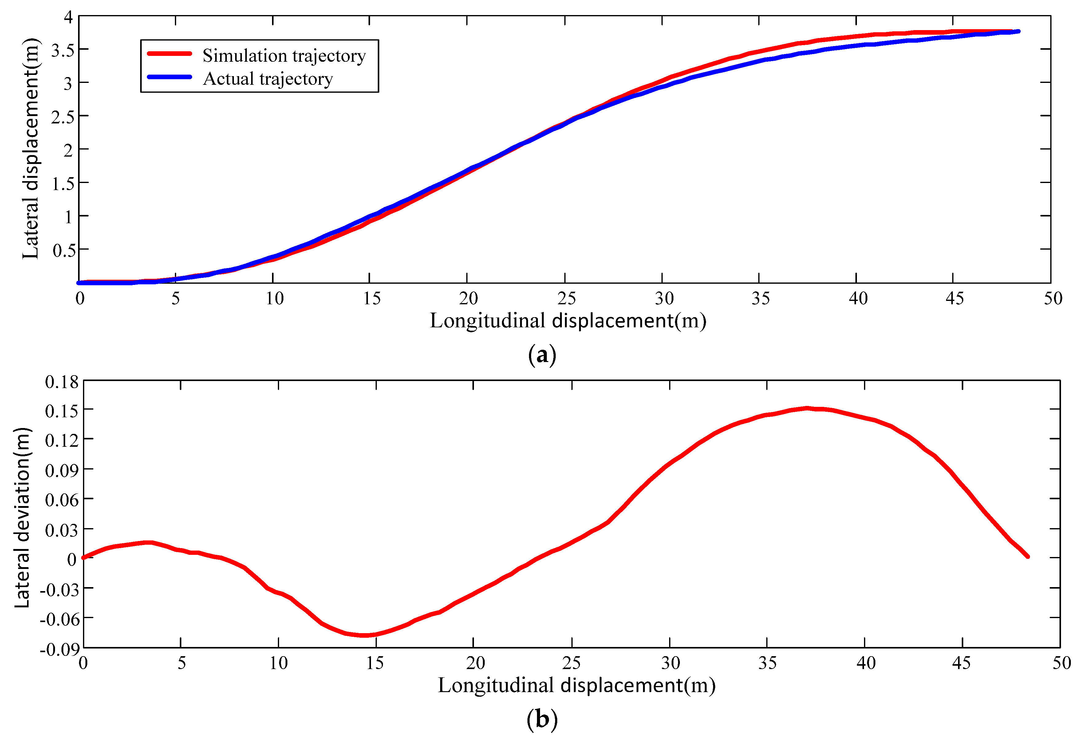
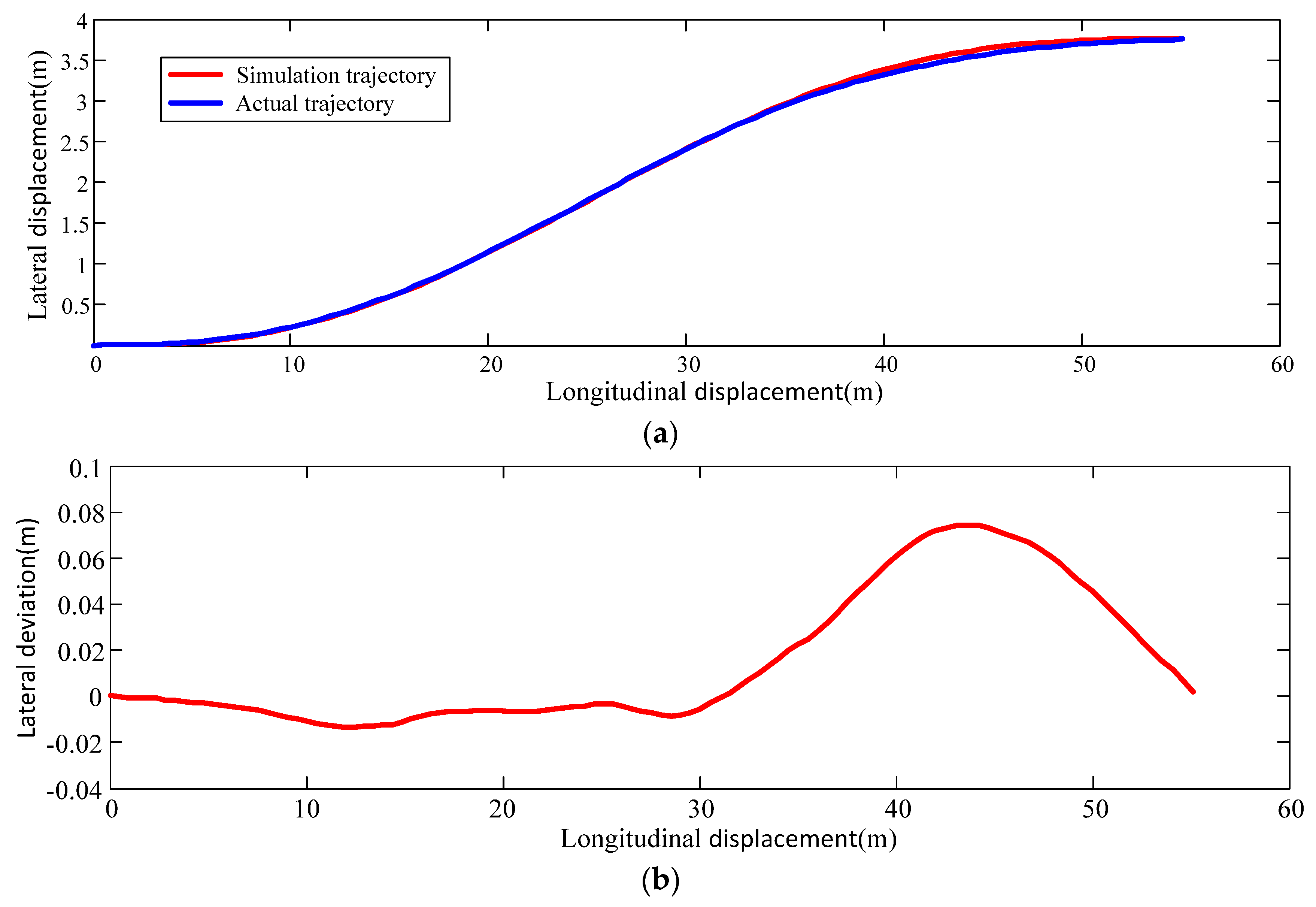
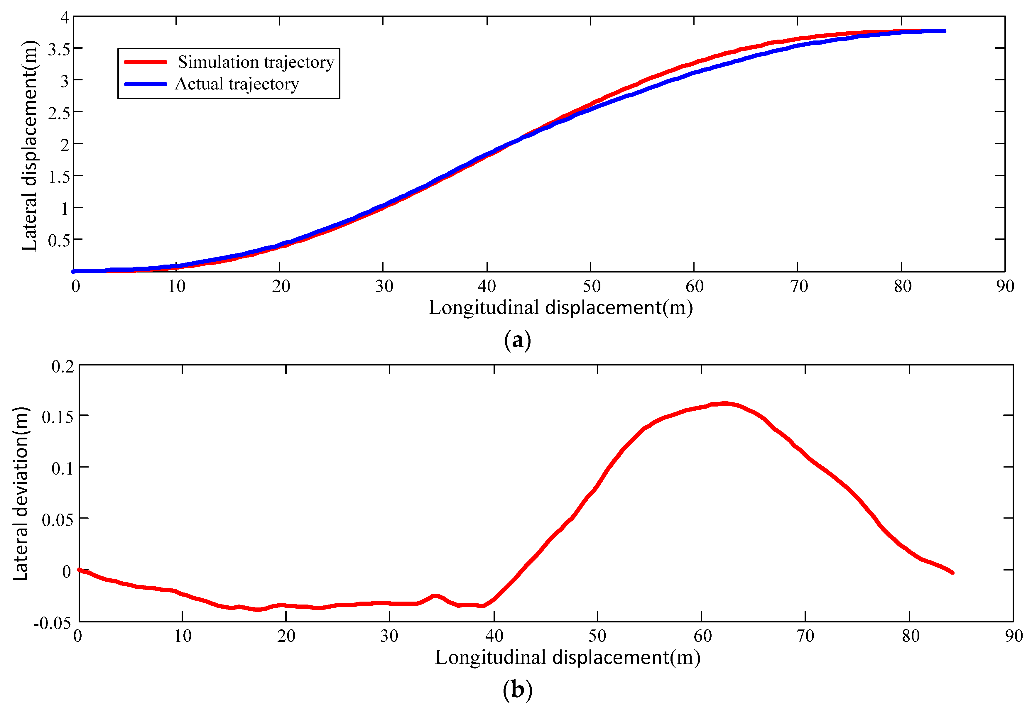
Figure 12 and Figure 13 are the simulation results at the speed of 30 km/h under the obstacle avoidance conditions. Figure 12a shows the simulation trajectory and actual trajectory of the conservative driver under the obstacle avoidance conditions. Figure 13a shows the trajectory of the aggressive driver. The red curve represents the lane-changing track obtained by the lane-changing path generation algorithm proposed in this paper. The blue curve represents the actual running track recorded in the real vehicle lane-changing test under the same condition. It can be seen in Figure 12a and Figure 13a that the trajectory obtained from simulation is basically consistent with the trajectory in real vehicle testing. It also meets the requirements of vehicle safety obstacle avoidance. Figure 12b and Figure 13b are the lateral error between the simulated and real trajectories of conservative drivers and aggressive drivers. The maximum lateral deviations are 0.056 m and 0.17 m, respectively. It means that the algorithm developed in this paper is with high accuracy and imitate the lane-changing operation of excellent drivers.
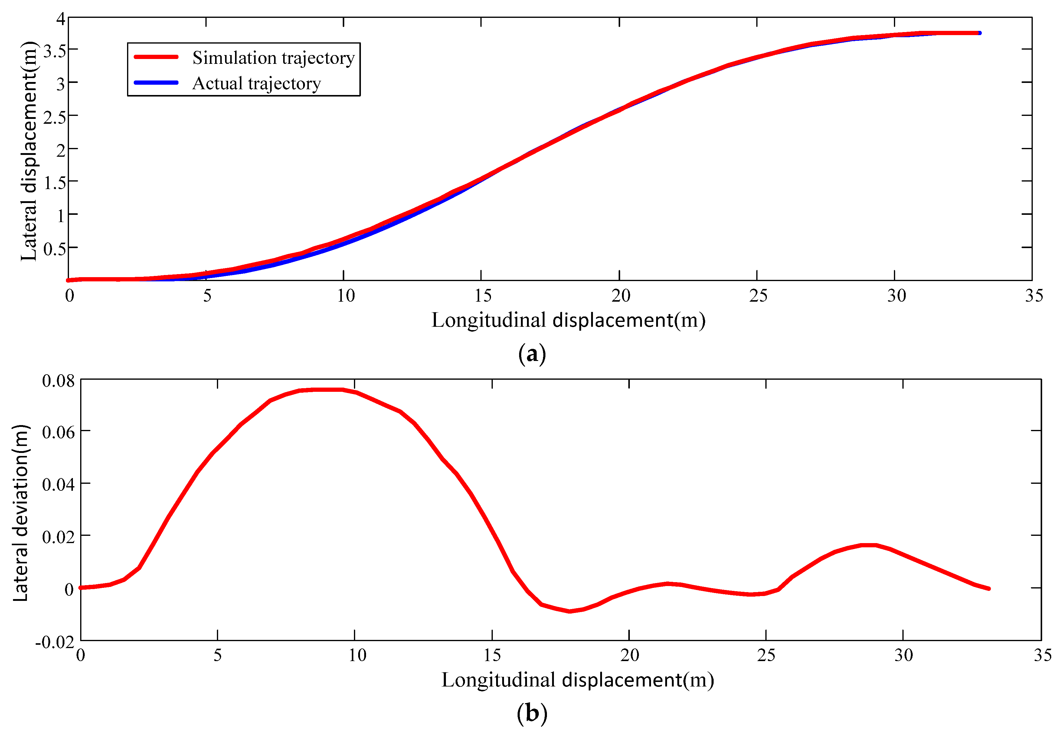
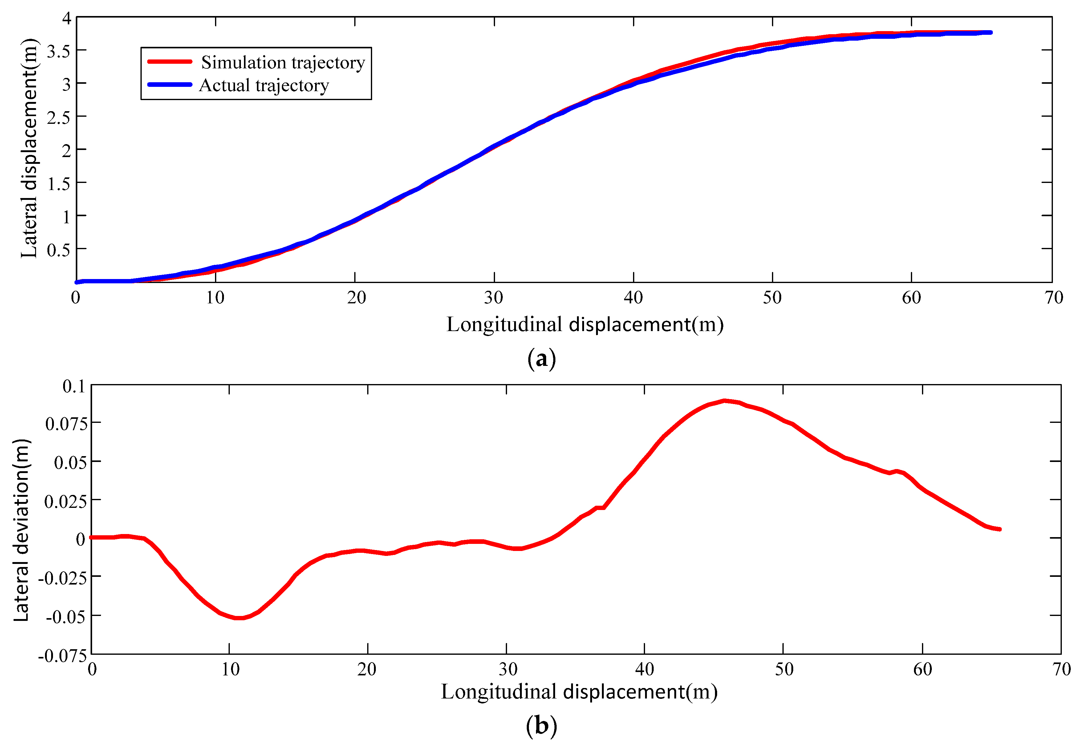
Figure 14 and Figure 15 are the simulation results at the speed of 40 km/h under the obstacle avoidance conditions. Figure 14a shows the simulation trajectory and actual trajectory of the conservative driver under the obstacle avoidance conditions. Figure 15a shows the two paths of the aggressive driver. Figure 14a and Figure 15a show that the simulation path and the actual path are very close to each other. It means the simulation trajectory can reflect the characteristics of excellent drivers’ lane-changing trajectories under the same working conditions. Figure 14b and Figure 15b are the lateral deviation between the simulated and real trajectories of conservative drivers and aggressive drivers at the speed of 40 km/h. The maximum lateral deviations are 0.087 m and 0.075 m, respectively, which means the method can keep high accuracy with the increased speed.
As can be observed in Figure 12a, Figure 13a, Figure 14a and Figure 15a, the longitudinal distance of the lane-changing trajectory is increased with the increased speed, and the longitudinal distance of the conservative driver at the same speed is shorter than that of the aggressive driver at same speed. This is because, in the process of obstacle avoidance, the conservative drivers usually keep a larger safety distance, and a larger steering wheel angle will be input at the early stage of the lane-changing. Therefore, the vehicle will travel to the target lane as soon as possible. Aggressive drivers often choose a smaller safety distance, so the lane-changing operation is more stable, making the terminal distance of lane changing longer.
5.2. Free Lane-Changing Simulation
Free lane-changing simulation test conditions: The speed is 30 km/h and 40 km/h, respectively; lane width is 3.75 m; and there is no obstacle.
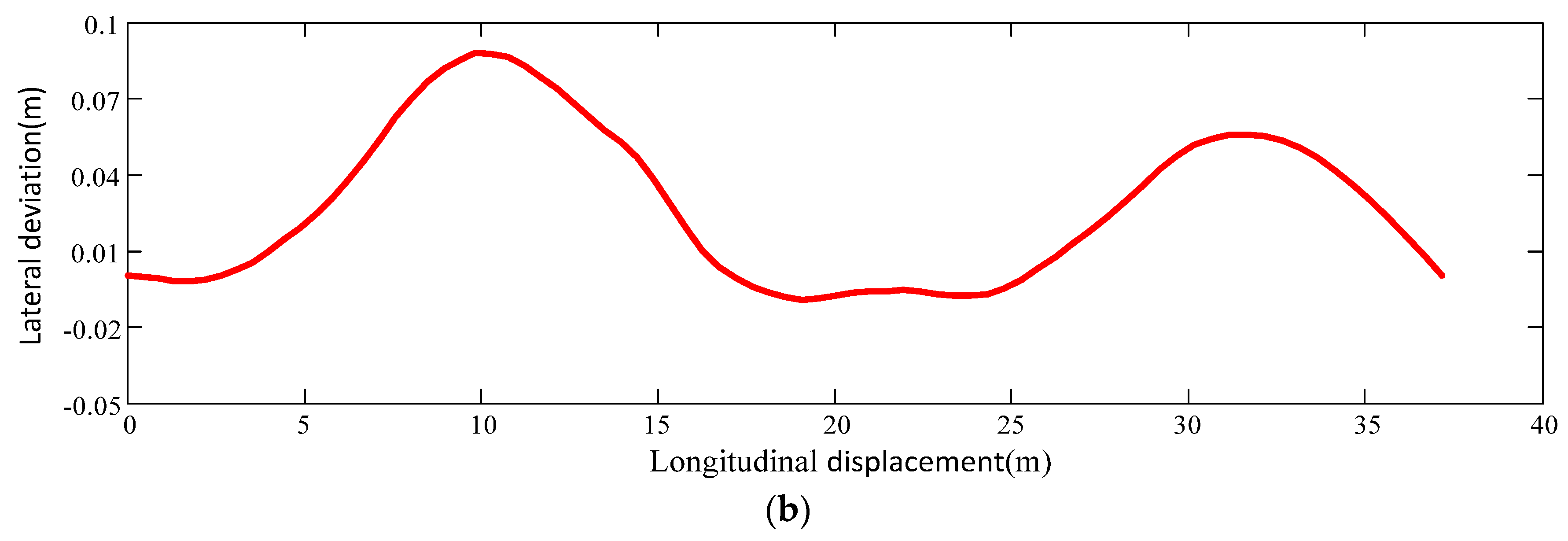
Figure 16 and Figure 17 are the simulation results at the speed of 30 km/h under the free lane-changing conditions. Figure 16a shows the simulation trajectory and actual trajectory of the aggressive driver under the free lane-changing conditions. Figure 17a shows the two trajectories of the conservative driver. The red curve represents the lane change track obtained by the lane-changing path generation algorithm proposed in this paper. The blue curve represents the test trajectory. In Figure 16a and Figure 17a, it can be seen that the coincidence of the trajectory obtained by the simulation and the actual trajectory of the test is high. Figure 16b and Figure 17b are the lateral error between the simulation and testing of aggressive drivers and conservative drivers, respectively. The maximum lateral deviations are 0.15 m and 0.074 m. Under the free lane-changing condition, the algorithm in this paper can also imitate the route of experienced drivers when do lane-changing operation.
Figure 18 and Figure 19 are the simulation results at the speed of 40 km/h under the free lane-changing conditions. Figure 18a shows the simulation trajectory and actual trajectory of the aggressive driver under the obstacle avoidance conditions. The two trajectories of the conservative driver at 40 km/h are presented in Figure 19a. The two diagrams show that the features of the route chosen by experienced driver can be represented by the simulation path. The lateral error between the simulation and test are shown in Figure 18b and Figure 19b. The maximum lateral deviations are 0.088 m and 0.16 m, respectively, which means the algorithm is with high accuracy under the free lane-changing condition.
In Figure 16a, Figure 17a, Figure 18a and Figure 19a, it can be seen the longitudinal distance chosen by the same type of drivers increases with the speed under the free lane-changing condition. However, the longitudinal distance chosen by the conservative driver under the free lane-changing condition is significantly longer than that of aggressive driver. Because a driver conducts the lane-changing operation according to his own habit when there is no obstacle under free condition, for the conservative driver, to reduce the lateral acceleration when changing lanes, the input steering wheel angle at the beginning of lane change will be reduced, which increases the longitudinal distance of the entire lane change, whereas, for aggressive drivers, they will choose to complete the lane change within shortest possible time, which requires a large steering wheel angle input, resulting in a smaller longitudinal distance of the lane-changing path.
6. Conclusions
A new lane-changing path planning method for unmanned vehicles is proposed in this paper. It is developed to generate a path that can make the vehicle finish the lane-changing operation smoothly and safely based on the information of vehicle speed, steering intention, obstacle and driving style. First, to obtain the lane-changing paths of the excellent drivers under different conditions, many real vehicle tests were carried out. Then, the final point and intermediate feature point of each lane change trajectory were extracted, with the expression of each path obtained. Next, the excellent driver model based on the GA-BP neural network was established and trained with experimental data. Finally, the path planning algorithm for imitating the lane-changing operation of excellent drivers was developed and presented.
The path developed in this paper can imitate real excellent driver lane-changing path to meet the kinematic constraints of the vehicle and avoid the obstacles at the same time. Simulation results verifies that the path planning method proposed in this research can generate an optimal lane-changing trajectory according to the vehicle driving condition and the driving styles selected by the passengers, which is basically the same with the trajectory selected by the excellent driver under the same conditions and the lateral error between the two trajectories is small. Therefore, the lane-changing path planning algorithm proposed in this paper can imitate the excellent driver to change the lane, improve the stability of the unmanned vehicle, improve the riding comfort of passengers, and reduce the probability of passengers suffering from motion sickness.
Author Contributions
G.G. and Z.W. conceived of and designed the method. G.G. and L.S. performed the experiments and analyzed the experimental data. Finally, Z.W. wrote the paper with the help of G.G., H.J. and C.D.
Acknowledgments
This work was financially supported by The National Natural Science Fund (No. U1564201 and No. 51675235), Six Talent Peaks Project Fund of Jiangsu Province (No. 2015-XNYQC-002), and Senior Talent Fund of Jiangsu University (No. 15JDG075).
Conflicts of Interest
The authors declare no conflict of interest.
References
- Rasekhipour, Y.; Khajepour, A.; Chen, S.K. A Potential Field-Based Model Predictive Path-Planning Controller for Autonomous Road Vehicles. IEEE Trans. Intell. Transp. Syst. 2017, 18, 1255–1267. [Google Scholar] [CrossRef]
- Korayem, M.H.; Nekoo, S.R. The SDRE control of mobile base cooperative manipulators: Collision free path planning and moving obstacle avoidance. Robot. Auton. Syst. 2016, 86, 86–105. [Google Scholar] [CrossRef]
- Gao, Y.Q.; Gray, A.; Tseng, H.E. A tube-based robust nonlinear predictive control approach to semiautonomous ground vehicles. Veh. Syst. Dyn. 2014, 52, 802–823. [Google Scholar] [CrossRef]
- Gao, Y.Q.; Lin, T.; Borrelli, F. Predictive Control of Autonomous Ground Vehicles With Obstacle Avoidance on Slippery Roads. In Proceedings of the ASME 2010 Dynamic Systems and Control Conference, Cambridge, MA, USA, 12–15 September 2010; pp. 265–272. [Google Scholar]
- Donatelli, M.; Giannelli, C.; Mugnaini, D. Curvature continuous path planning and path finding based on PH splines with tension. Comput. Aided Des. 2017, 88, 14–30. [Google Scholar] [CrossRef]
- Giannelli, C.; Mugnaini, D.; Sestini, A. Path planning with obstacle avoidance by G1 PH quintic splines. Comput. Aided Des. 2016, 76, 47–60. [Google Scholar] [CrossRef]
- Choi, J.W.; Curry, R.E.; Elkaim, G.H. Curvature-continuous trajectory generation with corridor constraint for autonomous ground vehicles. In Proceedings of the 49th IEEE Conference on Decision and Control, Hilton Atlanta Hotel, Atlanta, GA, USA, 15–17 December 2010; pp. 7166–7171. [Google Scholar]
- Meyer, G.; Beiker, S. Road Vehicle Automation 2; Springer International Publishing: Cham, Switzerland, 2015; ISBN 978-3-319-19077-8. [Google Scholar]
- Elbanhawi, M.; Simic, M.; Jazar, R. Improved maneuvering of autonomous passenger vehicles: Simulations and field results. J. Vib. Control 2017, 23, 1954–1983. [Google Scholar] [CrossRef]
- Diels, C.; Bos, J.E. Self-driving carsickness. Appl. Ergon. 2016, 53, 374–382. [Google Scholar] [CrossRef] [PubMed]
- Cao, P.; Hu, Y.; Miwa, T. An optimal mandatory lane change decision model for autonomous vehicles in urban arterials. J. Intell. Transp. Syst. 2017, 21, 271–284. [Google Scholar] [CrossRef]
- Butakov, V.A.; Ioannou, P. Personalized driver/vehicle lane change models for ADAS. IEEE Trans. Veh. Technol. 2015, 64, 4422–4431. [Google Scholar] [CrossRef]
- Nilsson, J.; Brännström, M.; Coelingh, E. Lane change maneuvers for automated vehicles. IEEE Trans. Intell. Transp. Syst. 2017, 18, 1087–1096. [Google Scholar] [CrossRef]
- Nilsson, J.; Brannstrom, M.; Coelingh, E. Longitudinal and lateral control for automated lane change maneuvers. In Proceedings of the American Control Conference, Palmer House Hilton, Chicago, IL, USA, 1–3 July 2015; pp. 1399–1404. [Google Scholar]
- Dubins, L.E. On Curves of Minimal Length with a Constraint on Average Curvature, and with Prescribed Initial and Terminal Positions and Tangents. Am. J. Math. 1957, 79, 497–516. [Google Scholar] [CrossRef]
- Lamiraux, F.; Lammond, J.P. Smooth motion planning for car-like vehicles. IEEE Trans. Robot. Autom. 2001, 17, 498–501. [Google Scholar] [CrossRef]
- Choi, Y.G.; Lim, K.I.; Kim, J.H. Lane change and path planning of autonomous vehicles using GIS. In Proceedings of the 12th International Conference on Ubiquitous Robots and Ambient Intelligence, KINTEX, Goyang, Korea, 28–30 October 2015; pp. 163–166. [Google Scholar]
- Ren, D.B.; Zhang, J.Y.; Zhang, J.M. Trajectory planning and yaw rate tracking control for lane changing of intelligent vehicle on curved road. Sci. China Technol. Sc. 2011, 54, 630–642. [Google Scholar] [CrossRef]
- Wang, C.; Zheng, C.Q. Lane change trajectory planning and simulation for intelligent vehicle. Adv. Mater. Res. 2013, 671, 2843–2846. [Google Scholar] [CrossRef]
- Yang, T.; Asanjan, A.A.; Faridzad, M. An enhanced artificial neural network with a shuffled complex evolutionary global optimization with principal component analysis. Inf. Sci. 2017, 418, 302–316. [Google Scholar] [CrossRef]
- Zhang, X.Y.; Yin, F.; Zhang, Y.M. Drawing and recognizing Chinese characters with recurrent neural network. IEEE Trans. Pattern Anal. Mach. Intell. 2018, 99, 849–862. [Google Scholar] [CrossRef] [PubMed]
- Jain, A.K.; Duin, R.P.W.; Mao, J. Statistical pattern recognition: A review. IEEE Trans. Pattern Anal. Mach. Intell. 2000, 22, 4–37. [Google Scholar] [CrossRef]
- Saon, G.; Soltau, H.; Nahamoo, D. Speaker adaptation of neural network acoustic models using i-vectors. In Proceedings of the IEEE Workshop on Automatic Speech Recognition and Understanding (ASRU), Olomouc, Czech Republic, 8–13 December 2013; pp. 55–59. [Google Scholar]
- Li, J.C.; Zhao, D.L.; Ge, B.F. A link prediction method for heterogeneous networks based on BP neural network. Physics A 2017, 495, 1–17. [Google Scholar] [CrossRef]
- Sharifian, A.; Ghadi, M.J.; Ghavidel, S. A new method based on Type-2 fuzzy neural network for accurate wind power forecasting under uncertain data. Renew. Energy 2018, 120, 220–230. [Google Scholar] [CrossRef]
- Xue, H.; Bai, Y.; Hu, H. Influenza activity surveillance based on multiple regression model and artificial neural network. IEEE Access. 2018, 6, 563–575. [Google Scholar] [CrossRef]
- Al-Qutami, T.A.; Ibrahim, R.; Ismail, I. Virtual multiphase flow metering using diverse neural network ensemble and adaptive simulated annealing. Expert Syst. Appl. 2018, 93, 72–85. [Google Scholar] [CrossRef]
- Yu, F.; Xu, X.Z. A short-term load forecasting model of natural gas based on optimized genetic algorithm and improved BP neural network. Appl. Energy 2014, 134, 102–113. [Google Scholar] [CrossRef]
- Wang, S.X.; Zhang, N.; Wu, L. Wind speed forecasting based on the hybrid ensemble empirical mode decomposition and GA-BP neural network method. Renew. Energy 2016, 94, 629–636. [Google Scholar] [CrossRef]
- Bin, W.; Zhu, X.; Shen, J. Analysis of driver emergency steering lane changing behavior based on naturalistic driving data. J. Tongji Univ. 2017, 45, 554–561. [Google Scholar]
Figure 1.
Test vehicle.

Figure 2.
Single lane change test.

Figure 3.
Relationships between the three different coordinate systems.

Figure 4.
The schematic diagram of the lane-changing path.

Figure 5.
The framework of the path planning method for imitating the lane-changing operation of excellent drivers.
Figure 5.
The framework of the path planning method for imitating the lane-changing operation of excellent drivers.

Figure 6.
Flow chart of GA-BP neural network algorithm.

Figure 7.
The lane-changing paths of different drivers at the same speed.

Figure 8.
The lane-changing paths with different intention.

Figure 9.
The lane-changing paths of one driver at different speeds.

Figure 10.
The testing error of the GA-BP neural network.

Figure 11.
The mean square error variation curve of the GA-BP neural networks model.

Figure 12.
The simulation results at the speed of 30 km/h under the obstacle avoidance conditions of the conservative driver: (a) simulation trajectory and actual trajectory; and (b) lateral deviations between the simulated and real trajectories.
Figure 12.
The simulation results at the speed of 30 km/h under the obstacle avoidance conditions of the conservative driver: (a) simulation trajectory and actual trajectory; and (b) lateral deviations between the simulated and real trajectories.

Figure 13.
The simulation results at the speed of 30 km/h under the obstacle avoidance conditions of the aggressive driver: (a) simulation trajectory and actual trajectory; and (b) lateral deviations between the simulated and real trajectories.
Figure 13.
The simulation results at the speed of 30 km/h under the obstacle avoidance conditions of the aggressive driver: (a) simulation trajectory and actual trajectory; and (b) lateral deviations between the simulated and real trajectories.

Figure 14.
The simulation results at the speed of 40 km/h under the obstacle avoidance conditions of the conservative driver: (a) simulation trajectory and actual trajectory; and (b) lateral deviations between the simulated and real trajectories.
Figure 14.
The simulation results at the speed of 40 km/h under the obstacle avoidance conditions of the conservative driver: (a) simulation trajectory and actual trajectory; and (b) lateral deviations between the simulated and real trajectories.


Figure 15.
The simulation results at the speed of 30 km/h under the obstacle avoidance conditions of the aggressive driver: (a) simulation trajectory and actual trajectory; and (b) lateral deviations between the simulated and real trajectories.
Figure 15.
The simulation results at the speed of 30 km/h under the obstacle avoidance conditions of the aggressive driver: (a) simulation trajectory and actual trajectory; and (b) lateral deviations between the simulated and real trajectories.

Figure 16.
The simulation results at the speed of 30 km/h under the free lane-changing conditions of the aggressive driver: (a) simulation trajectory and actual trajectory; and (b) lateral deviations between the simulated and real trajectories.
Figure 16.
The simulation results at the speed of 30 km/h under the free lane-changing conditions of the aggressive driver: (a) simulation trajectory and actual trajectory; and (b) lateral deviations between the simulated and real trajectories.

Figure 17.
The simulation results at the speed of 30 km/h under the free lane-changing conditions of the conservative driver: (a) simulation trajectory and actual trajectory; and (b) lateral deviations between the simulated and real trajectories.
Figure 17.
The simulation results at the speed of 30 km/h under the free lane-changing conditions of the conservative driver: (a) simulation trajectory and actual trajectory; and (b) lateral deviations between the simulated and real trajectories.

Figure 18.
The simulation results at the speed of 40 km/h under the free lane-changing conditions of the aggressive driver: (a) simulation trajectory and actual trajectory; and (b) lateral deviations between the simulated and real trajectories.
Figure 18.
The simulation results at the speed of 40 km/h under the free lane-changing conditions of the aggressive driver: (a) simulation trajectory and actual trajectory; and (b) lateral deviations between the simulated and real trajectories.

Figure 19.
The simulation results at the speed of 40 km/h under the free lane-changing conditions of the conservative driver: (a) simulation trajectory and actual trajectory; and (b) lateral deviations between the simulated and real trajectories.
Figure 19.
The simulation results at the speed of 40 km/h under the free lane-changing conditions of the conservative driver: (a) simulation trajectory and actual trajectory; and (b) lateral deviations between the simulated and real trajectories.


Table 1.
Information of drivers.
| Driver Number | Gender | Age | Driving Age (Years) |
|---|---|---|---|
| Driver 1 | Female | 55 | 33 |
| Driver 2 | Male | 28 | 10 |
| Driver 3 | Male | 53 | 31 |
| Driver 4 | Male | 46 | 22 |
| Driver 5 | Male | 53 | 21 |
Table 2.
Information of experiment data.
| Classification | Information |
|---|---|
| Number of drivers | 5 |
| Velocity (km/h) | 30, 35, 40, 45, 50 |
| Distance from obstacle (m) | 30, 35, 40, 45, 50, 55, 60, 65, 70, 75, 80, 100 (no obstacle) |
© 2018 by the authors. Licensee MDPI, Basel, Switzerland. This article is an open access article distributed under the terms and conditions of the Creative Commons Attribution (CC BY) license (http://creativecommons.org/licenses/by/4.0/).
Share and Cite
MDPI and ACS Style
Geng, G.; Wu, Z.; Jiang, H.; Sun, L.; Duan, C. Study on Path Planning Method for Imitating the Lane-Changing Operation of Excellent Drivers. Appl. Sci. 2018, 8, 814. https://0-doi-org.brum.beds.ac.uk/10.3390/app8050814
AMA Style
Geng G, Wu Z, Jiang H, Sun L, Duan C. Study on Path Planning Method for Imitating the Lane-Changing Operation of Excellent Drivers. Applied Sciences. 2018; 8(5):814. https://0-doi-org.brum.beds.ac.uk/10.3390/app8050814
Chicago/Turabian StyleGeng, Guoqing, Zhen Wu, Haobin Jiang, Liqin Sun, and Chen Duan. 2018. "Study on Path Planning Method for Imitating the Lane-Changing Operation of Excellent Drivers" Applied Sciences 8, no. 5: 814. https://0-doi-org.brum.beds.ac.uk/10.3390/app8050814
Note that from the first issue of 2016, this journal uses article numbers instead of page numbers. See further details here.