Towards Online Estimation of Human Joint Muscular Torque with a Lower Limb Exoskeleton Robot

Abstract

Exoskeleton robots demonstrate promise in their application in assisting or enhancing human physical capacity. Joint muscular torques (JMT) reflect human effort, which can be applied on an exoskeleton robot to realize an active power-assist function. The estimation of human JMT with a wearable exoskeleton is challenging. This paper proposed a novel human lower limb JMT estimation method based on the inverse dynamics of the human body. The method has two main parts: the inverse dynamic approach (IDA) and the sensing system. We solve the inverse dynamics of each human leg separately to shorten the serial chain and reduce computational complexity, and divide the JMT into the mass-induced one and the foot-contact-force (FCF)-induced one to avoid switching the dynamic equation due to different contact states of the feet. An exoskeleton embedded sensing system is designed to obtain the user’s motion data and FCF required by the IDA by mapping motion information from the exoskeleton to the human body. Compared with the popular electromyography (EMG) and wearable sensor based solutions, electrodes, sensors, and complex wiring on the human body are eliminated to improve wearing convenience. A comparison experiment shows that this method produces close output to a motion analysis system with different subjects in different motion.

1. Introduction

Exoskeleton robots demonstrate promise in their application in assisting or enhancing human physical capacity [1,2,3,4]. Estimating the intention of the user is fundamental for collaborative control of such wearable robots [5,6,7,8,9]. For an intention-based, active, power-assist exoskeleton, such as the Hybrid Assistive Limb (HAL) [10] from Tsukuba University and the Soft Exosuit [4] form Harvard University, a estimation of human effort is required by the controller to actively generate and exert assistive force/torque onto the human body. In fact, the joint muscular torque (JMT) reflects the human effort of each joint [2]. It not only indicates the direction in which the human tends to move the limbs, but also reflects the intensity of the effort. Previous research has confirmed the effectiveness of using JMT for active power-assist control with various kinds of exoskeleton robots [11,12,13]. However, estimating JMT is challenging.

More recent research has focused on improving the portability, stability, and convenience of solutions for JMT estimation. Some pure mechanical walking assist exoskeletons have been developed for simplicity and practicability. Elastic elements and cams have been adopted in mechanical structures to mimic human joint torque in some motion patterns, such as walking and running. Through the use of this torque, the exoskeleton is able to help the human body to perform some specific motion. Cristian C. et al. designed a mechanical system to help users with a walking disability [14]. Collins SH et al. proposed an unpowered ankle exoskeleton to help with the reduction of the user’s metabolic rate during walking [3]. An orthotic knee-extension made use of the gravity balancing technique to compensate for the user’s body weight [15]. These simplified solutions are good for reducing the weight and cost, and increasing the reliability, but they are always not adaptable to complex and changeable motion patterns, because the JMT of the human body changes during different motions, and the mismatch of the torque curve can lead to motion interference. A general solution is required to support the voluntary motion of a human body. There are two general methods for JMT estimation: (1) the electromyography (sEMG) based biological method, and (2) the inverse dynamics approach (IDA) based physics solution.

sEMG is an intuitive biological signal for detecting muscle activity. Buchanan et al. estimated joint moments and muscle forces using sEMG signals and verified them with inverse dynamics [16]. HAL is a typical active power-assist exoskeleton that uses sEMG [2]. Electrodes are pasted on the human body to determine the sEMG of each muscle group, and muscle activities are estimated to derive JMT based on the HAL generated assistive torques. Many other exoskeletons also use sEMG [11,12,13,17]. However, some limitations of sEMG are still under research. For example, in [18], it was concluded that sEMG is susceptible to the variation of electrode–skin conductivity, positioning, muscle fatigue and interactions between nearby muscles, so calibration is always required which increases the inconvenience of this method’s use. Complex wiring on the human body also influences its wearing convenience.

IDA has been successfully applied in clinical gait analysis. In Ref. [19], IDA was adopted to calculate human JMT during sit-to-stand movement. In Ref. [20], a motion capture system and several force plates were used to sense motion information and foot contact force (FCF). The entire clinical gait analysis system is universal but lacks portability. Hence, many wearable solutions have been proposed in recent years. Goniometers, inertial measurement units (IMUs), and air bladder based ground reaction force (GRF) measurement insoles are commonly used for human kinematic and kinetic measurements [21,22]. The problem is that it is difficult to precisely locate the wearable sensors and maintain stability on the soft tissue of the human body. Insoles with air bladders have always been always adopted to detect foot contact state, but it is difficult to get a precise GRF, because uneven distortion during complex foot–ground contact states leads to nonlinearity. In addition, the horizontal GRF cannot be measured by the insole either, which can cause error during joint torque estimation. Suin Kim et al. [23] proposed a wearable sensing system including IMUs and GRF measurement insoles to estimate the JMT in the sagittal plane. T. Liu et al. [24] developed a mobile force plate and motion analysis units to estimate 3D JMT. These devices are specifically designed to acquire the motion data of a human body, but are used to control an exoskeleton robot; thus, both the motion data of the user and the robot itself are required. It is unnecessary to introduce two sensing systems to measure the motion information of the user and the exoskeleton, respectively.

An exoskeleton embedded sensing system has the potential to collect motion data from the user, but few have taken advantage of this. H. Kazerooni et al. developed Berkeley Lower Extremity Exoskeleton (BLEEX) with integrated linear position sensor and foot pressure sensors [25]. They focused on minimizing human–exoskeleton interaction forces. They did not fully investigate the estimation of JMT using those embedded sensors. Researchers also developed the manipulator based human stiffness features learning method [26]. Saccares et al. designed another embedded sensing system [27]. They used the positions of the exoskeleton thigh and shank, and ground reaction forces on human feet in their simplified static shank equilibrium method (SSE) to calculate the torque command to the knee joints. B. Hwang et al. developed rehabilitation exoskeletons to measure the user’s JMT. In this method, the required joint torques of both the human body and the exoskeleton are calculated by inverse dynamics, respectively. The JMT is derived by removing the required joint torque of both the exoskeleton and the human limbs from the measured joint torque by torque sensors in the exoskeleton joints. The method in Ref. [28] is valid only during swing motion, and was improved in reference [29]. An insole sensor with air bladders was introduced to measure the GRF, which extends their method to the stance phase. However, the insole cannot measure the horizontal GRF. This may lead to estimation error. Besides, the influence of hip acceleration was not discussed.

This work presents a novel implementation of the human lower limb JMT estimation method to devise an online JMT estimation solution that can be used to achieve active power-assist function on our prototype active power-assist lower limb exoskeleton (APAL) [30]. The main achievement of this paper is the design of an embedded sensing system and a specially designed inverse dynamics process. The sensing system is integrated in the exoskeleton structure which does not mount any sensors on the human body but obtains the motion data and interaction forces of the human body by mapping motion from the exoskeleton to a human model. Unlike traditional IDA, we solve the inverse dynamics of each human leg separately to shorten the serial chain and reduce the computational complexity. The JMT is divided into two parts which we call the mass-induced one and the FCF-induced one to avoid discontinuous dynamic equations due to different contact states of feet.

The rest of the paper is organized as follows. Section 2 presents a parameterized model of the human body and specially designed inverse dynamics for estimating JMT, and then presents the embedded sensing system including trunk posture, joint motion information, and foot contact force. Section 3 demonstrates and discusses the results of the JMT estimation experiments. Finally, the conclusions of this paper are presented in Section 4.

2. Methods

Human JMT cannot be measured directly, but within the framework of Newtonian mechanics, the interaction forces/torques in a rigid body system can be deduced from the motion information and external forces acting on it. This notion holds for the human body. For application to the control of an exoskeleton robot, a novel sensing system and the relevant IDA are designed to meet the requirements of portability and simplicity.

2.1. Parameterized Model of the Human Body

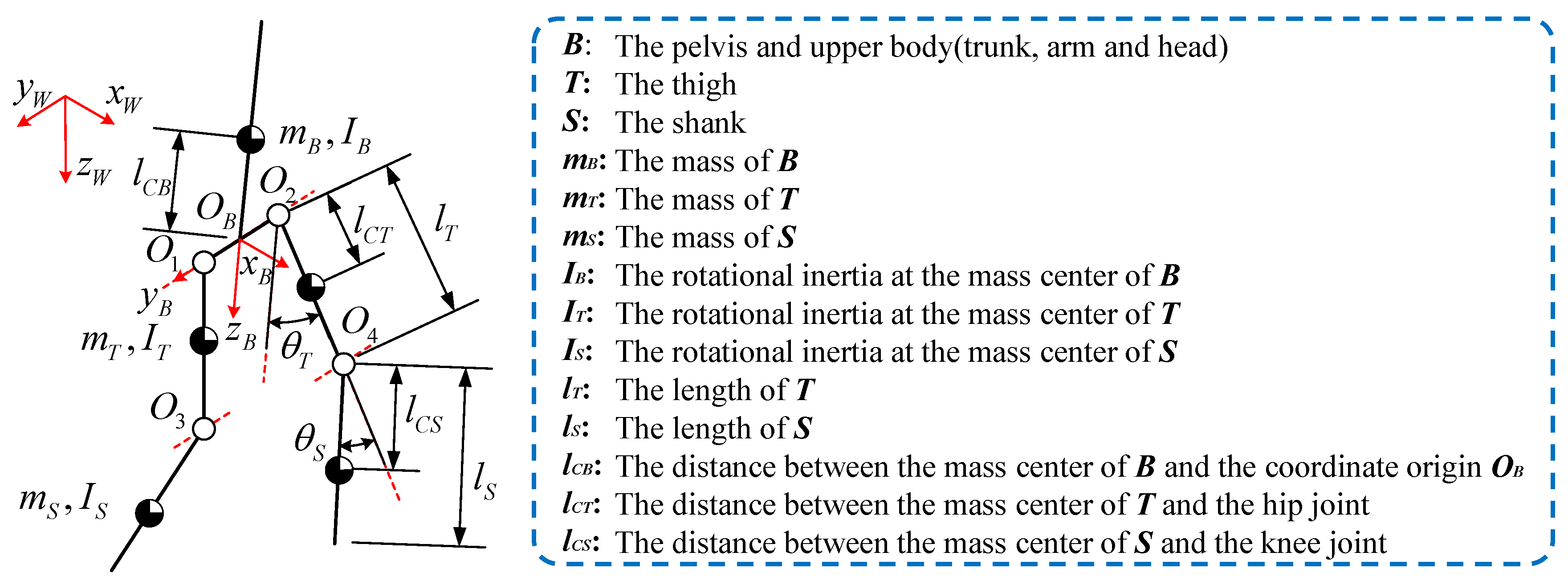
As shown in Figure 1, a parameterized model of a human body was adopted to solve the IDA in the sagittal plane. In this method, the human body is represented by a 5-bar model. There have been many relevant discussions about the calculation of body dimensions and inertial parameters. In Ref. [31,32], quadratic regression equations are presented to derive different subjects’ individual parameters using only his/her weight and height.

2.2. Inverse Dynamics of the Human Body

Generally, the human walking process includes several states, such as (i) single support, (ii) double support, and (iii) double off-the-ground. Dynamic models of these states are also different due to different constraints on the feet. Commonly, a finite-state-machine (FSM) should be employed to switch between the dynamic equations of each state. However, this can increase the complexity of the control algorithm for state classification.

To solve the JMT, this model considers the dynamics of each leg separately, instead of treating the dynamics of the human body as a whole, thereby shortening the kinematic chain from the 5-bar model of the entire body to a 2-bar model of each leg. This helps to reduce the computational complexity and local disturbances. In inverse dynamic formulas of joint torque, there are several components, including torques caused by inertial, coriolis, gravity, and external forces. Each component is linearly added. So, we are able to further factorize the inverse dynamics of a single leg into the mass-induced one and FCF-induced one. This helps to avoid switching dynamic equations due to different contact states of the feet.

The proposed method is limited by several assumptions: (1) it only investigates motion in the sagittal plane for simplicity, thereby neglecting motion and force in the coronal plane and the frontal plane; (2) inertial torque caused by ankle movement is neglected; and (3) the foot and shank are considered as one component in the human model during the swing phase.

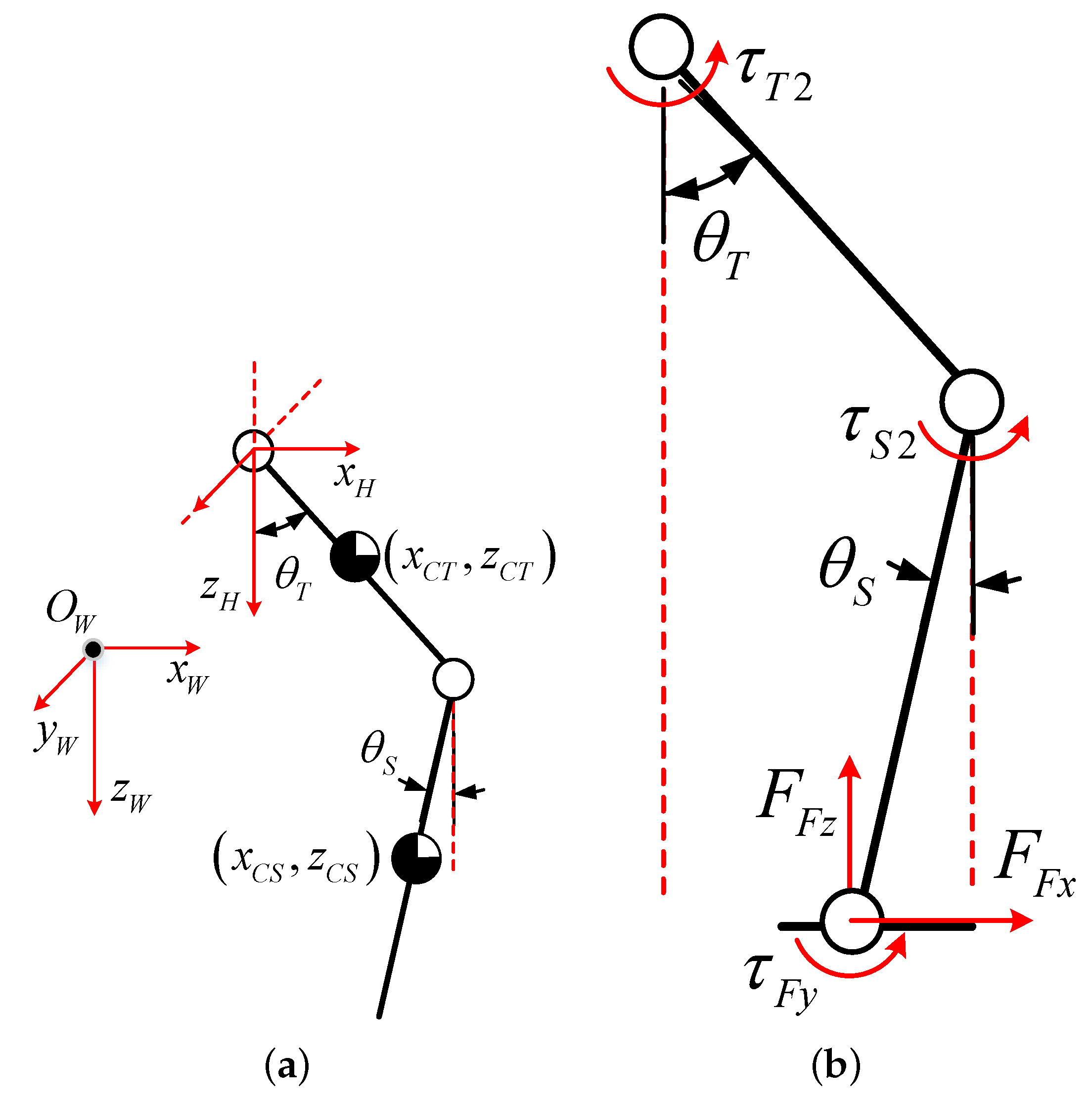
In the estimation of mass-induced torques, the leg is considered to be suspended to component B by the hip joint where the coordinate origin is set as shown in Figure 2a. The Lagrange method is adopted on this two-bar dynamic model with floating pedestals. First, the coordinates of the center of mass of component T are determined in the global coordinate system $O_W$.

$$\left\{\begin{array}{c}{x}_{CT}=x_H+l_{CT}sin\left({\theta }_T\right)\hfill \\ z_{CT}=z_H+l_{CT}cos\left({\theta }_T\right).\hfill \end{array}\right.$$

(1)

Next, the motion velocity of the center of mass for component T is derived:

$$\left\{\begin{array}{c}{\dot{x}}_{CT}=\frac{\partial x_{CT}}{\partial x_H}{\dot{x}}_H+\frac{\partial x_{CT}}{\partial {\theta }_T}{\dot{\theta }}_T\hfill \\ {\dot{z}}_{CT}=\frac{\partial z_{CT}}{\partial z_H}{\dot{x}}_H+\frac{\partial z_{CT}}{\partial {\theta }_T}{\dot{\theta }}_T.\hfill \end{array}\right.$$

(2)

Then, the coordinates of the center of mass for component S in the global coordinate system $O_W$ are derived:

$$\left\{\begin{array}{c}{x}_{CS}=x_H+l_{T}sin\left({\theta }_T\right)+l_{CS}sin\left({\theta }_S\right)\hfill \\ z_{CS}=z_H+l_{T}cos\left({\theta }_T\right)+l_{CS}cos\left({\theta }_S\right).\hfill \end{array}\right.$$

(3)

Next, the motion velocity of the center of mass for component S is derived:

$$\left\{\begin{array}{c}{\dot{x}}_{CS}=\frac{\partial x_{CS}}{\partial x_H}{\dot{x}}_H+\frac{\partial x_{CS}}{\partial {\theta }_T}{\dot{\theta }}_T+\frac{\partial x_{CS}}{\partial {\theta }_S}{\dot{\theta }}_S\hfill \\ {\dot{z}}_{CS}=\frac{\partial z_{CS}}{\partial z_H}{\dot{z}}_H+\frac{\partial z_{CS}}{\partial {\theta }_T}{\dot{\theta }}_T+\frac{\partial z_{CS}}{\partial {\theta }_S}{\dot{\theta }}_S.\hfill \end{array}\right.$$

(4)

Thereby, the total kinetic energy of the system is calculated:

$$K=\frac{1}{2}\left[m_T({\dot{x}}_{CT}^2+{\dot{z}}_{CT}^2)+m_S({\dot{x}}_{CS}^2+{\dot{z}}_{CS}^2)+I_T{\dot{\theta }}_T^2+I_S{\dot{\theta }}_S^2\right].$$

(5)

In addition, the potential energy of the system is calculated:

$$P=-m_{T}g{z}_T-m_{s}g{z}_s.$$

(6)

The, we get the equation of the mass-induced torque:

$$\left\{\begin{array}{c}{\tau }_{T1}=\frac{d}{dt}\left[\frac{\partial (K-P)}{\partial {\dot{\theta }}_T}\right]-\frac{\partial (K-P)}{\partial {\theta }_T}\hfill \\ {\tau }_{S1}=\frac{d}{dt}\left[\frac{\partial (K-P)}{\partial {\dot{\theta }}_S}\right]-\frac{\partial (K-P)}{\partial {\theta }_S}.\hfill \end{array}\right.$$

(7)

In the estimation of FCF-induced JMT, the human feet contacting the shoes and the upper end of the leg support the entire trunk. The JMTs are calculated via the force equilibrium equation, as shown in Figure 2b. The FCF values, including $F_{Fx}$, $F_{Fz}$ and ${\tau }_{Fy}$, are measured, and the force balance equations are solved to derive the hip and knee JMTs ${\tau }_{T2}$ and ${\tau }_{S2}$:

$$\left\{\begin{array}{c}{\tau }_{T2}=F_{Fx}(l_{T}cos\left({\theta }_T\right)+l_{S}cos\left({\theta }_S\right))+F_{Fz}(l_{T}sin\left({\theta }_T\right)-l_{S}sin\left({\theta }_S\right))+{\tau }_{Fy}\hfill \\ {\tau }_{S2}=F_{Fx}{l}_{S}cos\left({\theta }_S\right)-F_{Fz}{l}_{z}sin\left({\theta }_S\right)+{\tau }_{Fy}.\hfill \end{array}\right.$$

(8)

Finally, the mass- and FCF-induced JMTs are summed up and the total JMT of the hip and knee is derived:

$$\left\{\begin{array}{c}{\tau }_T={\tau }_{T_1}+{\tau }_{T_2}\hfill \\ {\tau }_S={\tau }_{S_1}+{\tau }_{S_2}.\hfill \end{array}\right.$$

(9)

2.3. Sensing System Design

A sensing system was designed to measure all signals required by the proposed IDA, including the posture of the trunk (B), the acceleration of hip joints ($O_1$ and $O_2$), the angular displacement/velocity/acceleration of the hip and knee joints, and the foot contact forces (FCF). To avoid misalignment of the sensor and user discomfort, the motion information of the human body is not measured directly by mounting sensors on the human body. Instead, the entire sensing system is embedded into the exoskeleton structure to get the motion information about the exoskeleton. Then, according to the motion mapping from the exoskeleton to the human model, the user’s motion data are derived. The motion mapping is ensured by the structural design, the description of which can be found in Ref. [30]. The sensing system is described below.

2.3.1. Overall Hardware Architecture

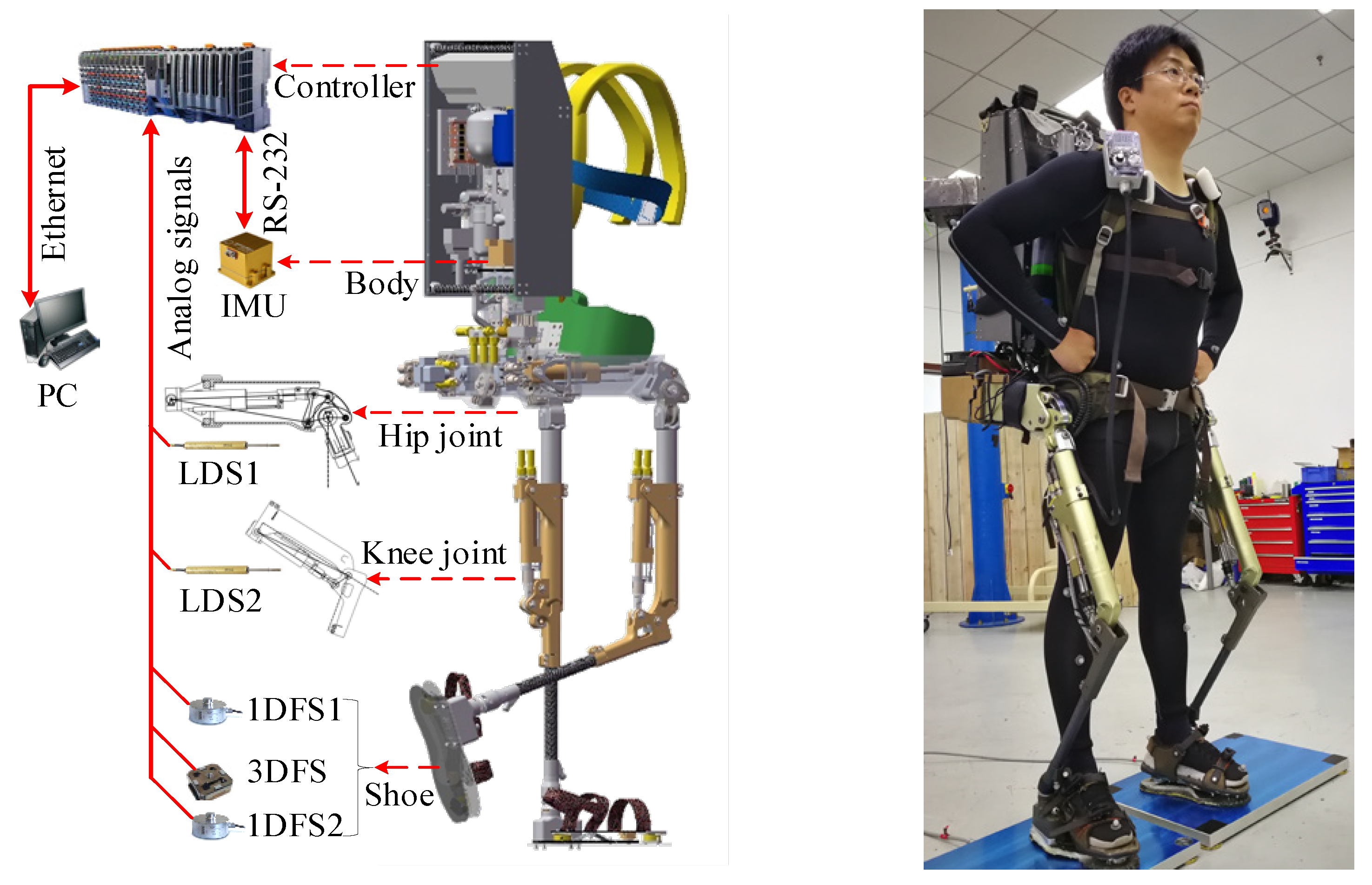
The active power-assist lower limb exoskeleton APAL [30] is introduced in Figure 3. The central controller is a $B\&R$ PLC (Programmable Logic Controller by $B\&R$ Industrial Automation GmbH, Eggelsberg, Austria). The inertial measurement unit (IMU) data are read by the PCL through the RS-232 bus. The linear displacement sensors (LDS) placed on the hip and knee joints, as well as 1D and 3D force sensors in the sole, are connected to an AD converter. The inverse dynamics are solved online in the PLC. An external PC records the result from the PLC in real-time via an ethernet bus.

2.3.2. Trunk Posture and Hip Joint Acceleration Measurements

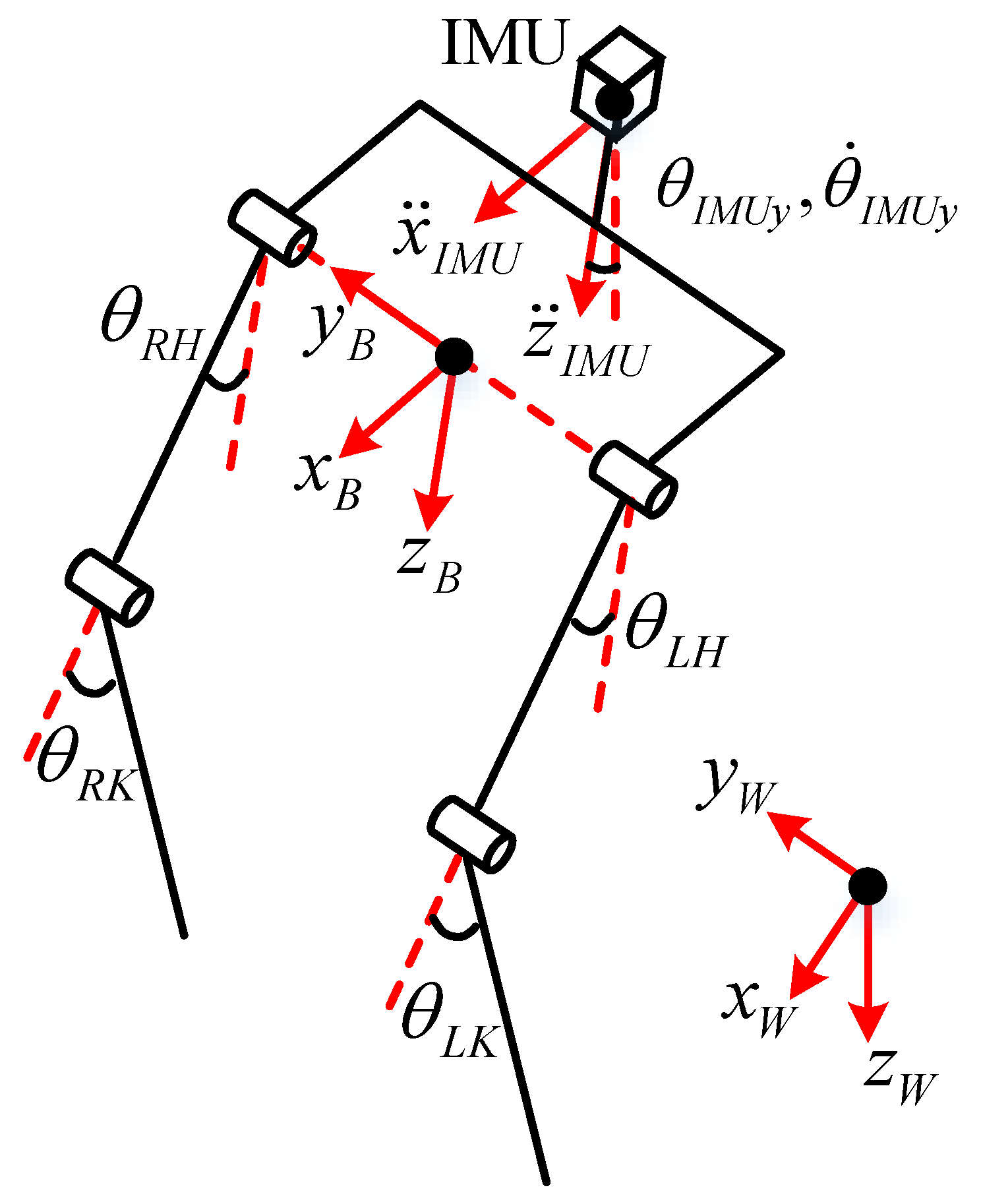
The human body is firmly connected to the exoskeleton via the trunk and feet, and a unique motion mapping from the exoskeleton to the human body is ensured by APAL kinematics and its structure design. Thus, we are able to derive motion data of the human body from the embedded sensing system in the exoskeleton. An IMU is adopted to measure the trunk posture and acceleration of the hip joints. As shown in Figure 4, the axis of the IMU is set parallel to the body coordinate axis, so IMU directly provides the attitude (${}^W{\mathit{\theta }}_{IMU}=\{{\theta }_{roll},{\theta }_{pitch},{\theta }_{yaw}\}$) in the world coordinate system (WCS), and the angular velocity (${{}^B\dot{\mathit{\theta }}}_{IMU}=\{{\omega }_{roll},{\omega }_{pitch},{\omega }_{yaw}\}$) and acceleration (${}^B{\mathit{a}}_{IMU}=\{{}^B{\ddot{x}}_{IMU},{}^B{\ddot{y}}_{IMU},{}^B{\ddot{z}}_{IMU}\}$) of the body coordinate system (BCS). The angular acceleration (${}^B{\ddot{\mathit{\theta }}}_{IMU}$) of the IMU in the BCS can be obtained via the first-order difference of ${}^B{\dot{\mathit{\theta }}}_{IMU}$. To improve the smoothness and reduce the high-frequency noise induced by quantization error, interpolation and a low pass filter are used.

For the trunk posture, since the IMU is fixed in the exoskeleton back frame which is securely connected to the human trunk, the posture of component B equals ${}^W{\mathit{\theta }}_{IMU}$. The acceleration $({}^W{\ddot{x}}_H,{}^W{\ddot{y}}_H,{}^W{\ddot{z}}_H)$ of the hip joint cannot be measured directly in the WCS by the IMU because $O_1$ and $O_2$ do not coincide with $O_B$, but they can be derived through kinematic relations. The acceleration (${}^B{\mathit{a}}_{IMU}$) obtained by the IMU is first converted from the BCS to the WCS as ${}^W{\mathit{a}}_{IMU}={}^{BtoW}\mathit{R}·{}^B{\mathit{a}}_{IMU}$, where ${}^{BtoW}\mathit{R}$ is the rotation matrix for the BCS–WCS conversion. Let the coordinates of the IMU in the BCS be ${}^B{\mathit{P}}_{IMU}$, and those in the WCS be ${}^W{\mathit{P}}_{IMU}$. Thus, the coordinates of the left hip joint in the BCS are ${}^B{\mathit{P}}_H$, and those in the WCS should be ${}^W{\mathit{P}}_H={}^{BtoW}\mathit{R}·({}^B{\mathit{P}}_H-{}^B{\mathit{P}}_{IMU})+{}^W{\mathit{P}}_{IMU}$. The acceleration in the WCS is ${}^W{\mathit{a}}_H={}^W{\ddot{\mathit{P}}}_H={}^{BtoW}\ddot{\mathit{R}}·({}^B{\mathit{P}}_H-{}^B{\mathit{P}}_{IMU})+{}^W{\mathit{a}}_{IMU}$. Here, ${}^{BtoW}\ddot{\mathit{R}}$ is the second-order differential of the rotation matrix (${}^{BtoW}\mathit{R}$). The required ${}^W{\ddot{x}}_H$ and ${}^W{\ddot{z}}_H$ are components of ${}^W{\mathit{a}}_H$ on axes $x_W$ and $z_W$, respectively.

2.3.3. Hip and Knee Joint Kinematics Information Measurement

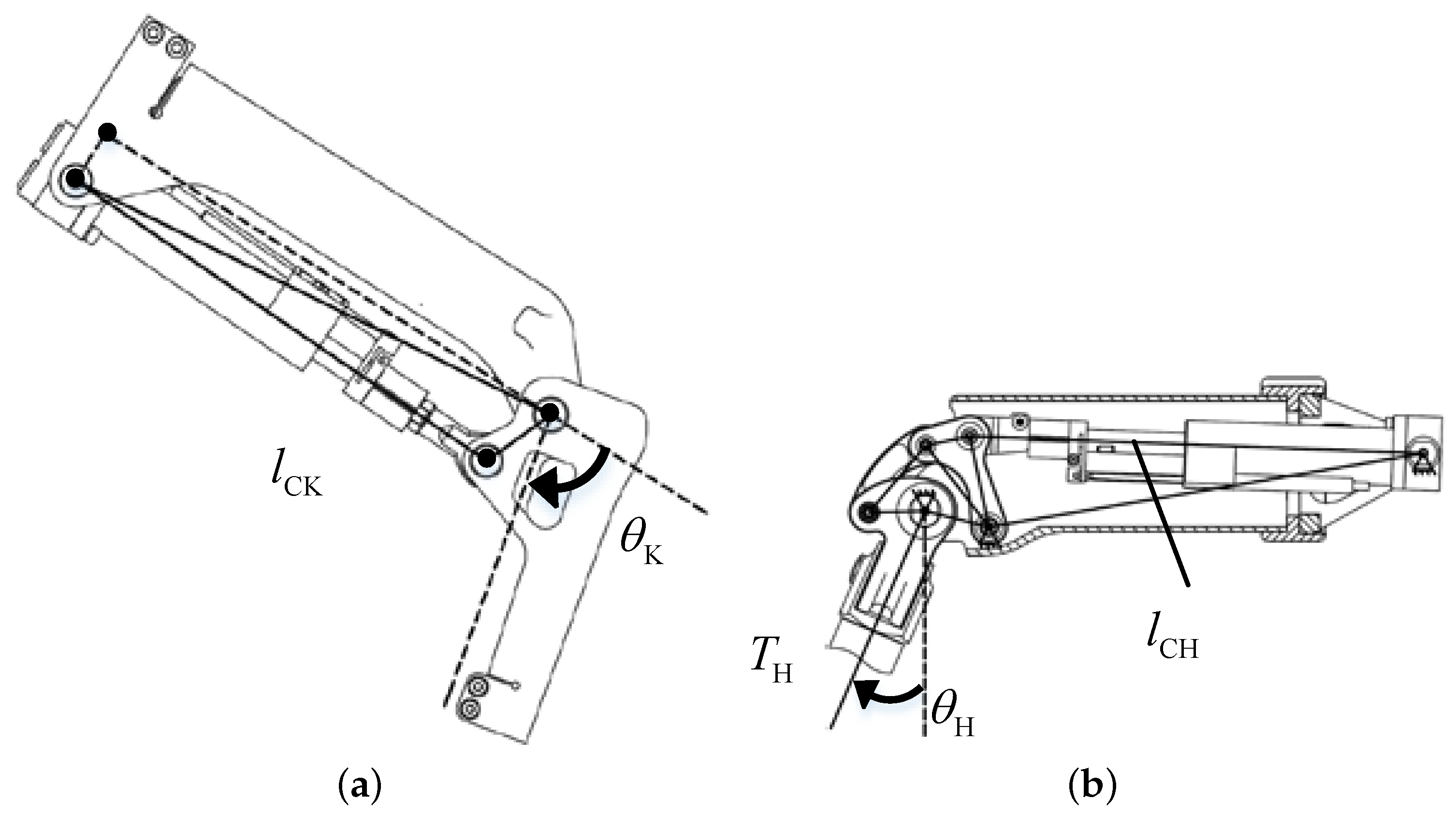
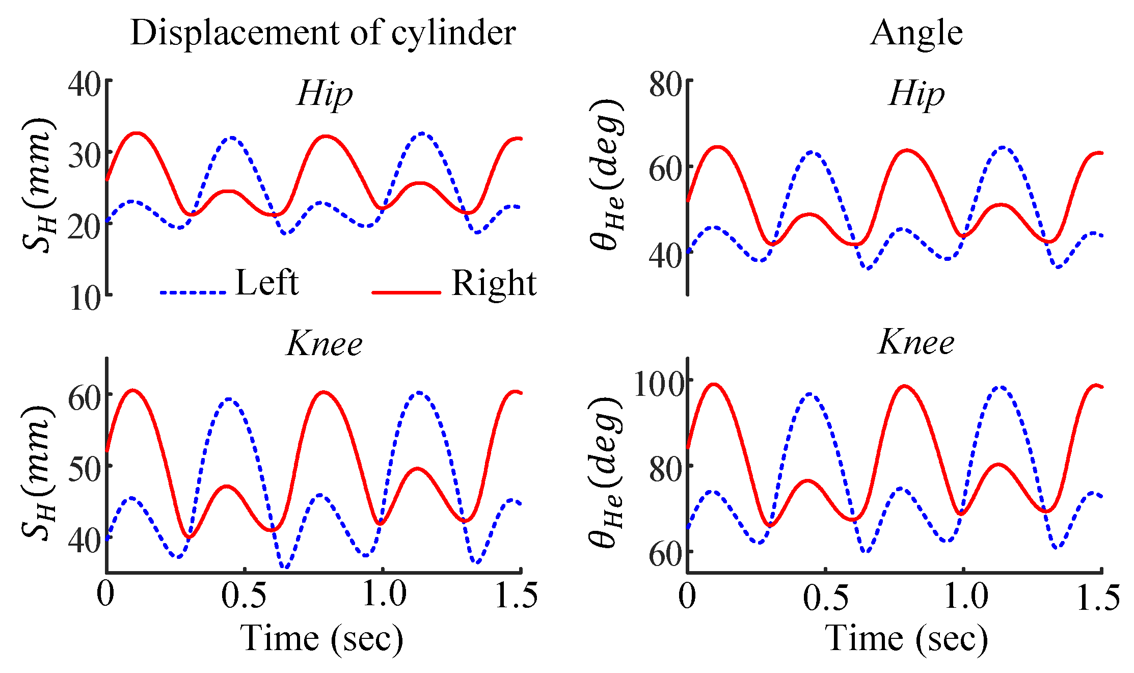
The angles of the hip and knee joints are derived from the respective measurements of the cylinder displacement of the exoskeleton. The displacement signals ($S_H$ and $S_K$) from LDSs are converted into hip and knee joint angles (${\theta }_H$ and ${\theta }_K$), according to the geometry of the joints, as shown in Figure 5. The angular velocities (${\dot{\theta }}_H$ and ${\dot{\theta }}_K$) are obtained via the first-order differences of ${\theta }_H$ and ${\theta }_K$. Similarly, the angular accelerations (${\ddot{\theta }}_H$ and ${\ddot{\theta }}_K$) are obtained from the first-order differential of ${\dot{\theta }}_H$ and ${\dot{\theta }}_K$.

The exoskeleton is design with its hip and ankle axes close to those of the user. The back frame and shoes are firmly connected to the user. So, we can assume that the coordinates of the exoskeleton ankle joints in the BCS are nearly the same as those of the human body. This can be expressed as follows:

$$\left\{\begin{array}{c}{x}_F=l_{Te}sin\left({\theta }_{He}\right)-l_{Se}sin({\theta }_{Ke}-{\theta }_{He})=l_{T}sin\left({\theta }_H\right)-l_{S}sin({\theta }_K-{\theta }_H)\hfill \\ z_F=l_{Te}cos\left({\theta }_{He}\right)+l_{Se}cos({\theta }_{Ke}-{\theta }_{He})=l_{T}cos\left({\theta }_H\right)+l_{S}cos({\theta }_K-{\theta }_H)\hfill \end{array}\right.$$

(10)

where ${\theta }_{He}$ and ${\theta }_{Ke}$ are the hip and knee joint angles of the exoskeleton; $l_{Te}$ and $l_{Se}$ are the lengths of the thigh and shank of exoskeleton, which are $450mm$ and $440mm$, respectively; and $l_T$ and $l_S$ are the lengths of components T and S of the simplified human model, which are $424mm$ and $422mm$, respectively. Equation (10) allows us to derive the joint angles of the human body (${\theta }_H$ and ${\theta }_K$), as well as ${\dot{\theta }}_H$, ${\dot{\theta }}_K$, ${\ddot{\theta }}_H$, and ${\ddot{\theta }}_K$.

2.3.4. Foot Contact Forces (FCFs) Measurements

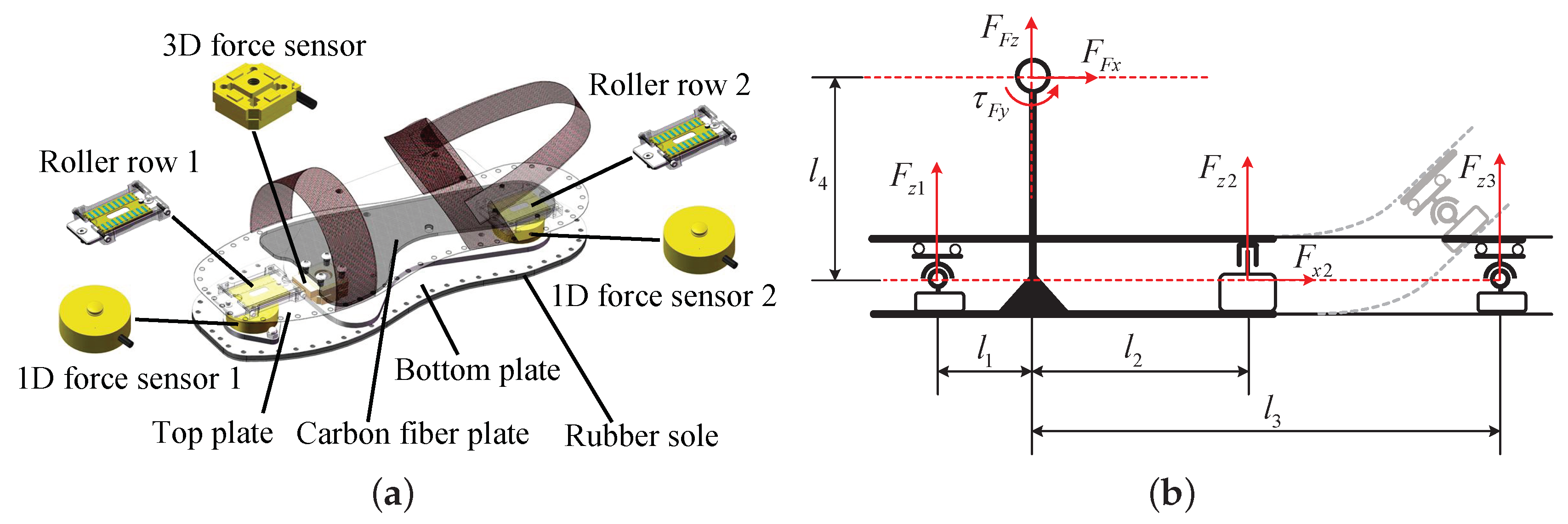
A special shoe was developed to measure FCF in the sagittal plane. Note that the FCF is an interaction force between the foot and shoe. It is different from GRF. GRFs only appear when the foot touches the ground, but FCFs exist in both the stance and swing phases. There are three components of FCF in the sagittal plane, which include $F_{Fx}$ in the front–rear direction, $F_{Fz}$ in the up–down direction, and torque $T_{Fy}$ on the dorsiflexion axis. The force condition of the sole is complex. There are many contact states of the sole during exercise, such as heel strike, full foot landing, forefoot landing, and toe landing, while ground unevenness can also cause unpredictable deformation of the sole. Moreover, rotational freedom of the human toe joint is required for walking stability and energy saving [33], so the sole should be flexible. Thus, a double-layer elastic steel sole structure was designed, as shown in Figure 6a.

The proposed design utilizes a combination of a 3D force sensor and two 1D force sensors. The 3D force sensor is arranged slightly behind the toe joint, and the sensor can obtain the up–down direction force ($F_{z2}$) and the front-rear direction force ($F_{x2}$). A 1D force sensor with a high overload margin is set under the heel to measure the GRF ($F_{z1}$) on the heel. A 1D force sensor is placed under the toe to measure the supporting force ($F_{z3}$). The sensor layout and force analysis model are shown in Figure 6b.

For computational purposes, the force signals obtained from the force sensors are synthesized to the ankle joint. The resultant forces can be calculated based on the location of the force sensors:

$$\left\{\begin{array}{c}{F}_{Fx}=F_{x2}\hfill \\ F_{Fz}=F_{z1}+F_{z2}+F_{z3}\hfill \\ {\tau }_{Fy}=F_{x2}{l}_4-F_{z1}{l}_1+F_{z2}{l}_2+F_{z3}{l}_3.\hfill \end{array}\right.$$

(11)

3. Experimental Results and Discussion

3.1. Motion Data Sampling and JMT Estimation

In this experiment, the user wearing the exoskeleton did ran in place with a stride frequency of approximately 2.8 Hz. The power unit of the exoskeleton was switched off and all joints were set free to avoid interference. The weight of the exoskeleton was assumed to be carried by the subject. The motion information of the human body was acquired by the embedded sensing system.The hip and knee JMTs were calculated by the controller of the exoskeleton and sent to a PC in real-time for recording and graphing. We had five subjects. Their parameters were calculated according to previous research [31,32] and are listed in

Table 1. Parameters of the simplified human model.

	H	M	${\mathit{m}}_{\mathit{T}}$	${\mathit{m}}_{\mathit{S}}$	${\mathit{I}}_{\mathit{T}}$	${\mathit{I}}_{\mathit{S}}$	${\mathit{l}}_{\mathit{T}}$	${\mathit{l}}_{\mathit{S}}$	${\mathit{l}}_{\mathit{CT}}$	${\mathit{l}}_{\mathit{CS}}$
	(m)	(kg)	(kg)	(kg)	(kg·mm${}^2$)	(kg·mm${}^2$)	(mm)	(mm)	(mm)	(mm)
S1	1.75	76.5	7.65	4.65	0.143	0.18	424	422	183	270
S2	1.64	60.3	6.03	3.67	0.099	0.124	397	395	172	253
S3	1.72	61.5	6.15	3.74	0.111	0.140	416	415	180	266
S4	1.78	78.5	7.85	4.77	0.152	0.192	431	429	187	275
S5	1.65	70.2	7.02	4.27	0.117	0.147	399	398	173	255

. Only subject 1 participated in this experiment.

(1)

The Posture of the Trunk

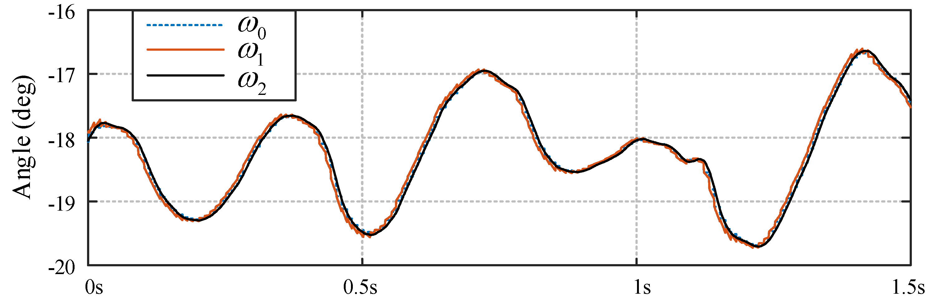
Since we only studied the motion in the sagittal plane, just the pitch angle was required. The maximal sample frequency of the IMU is 100 Hz. For smoother IDA, a higher sample frequency, e.g., 1 kHz is required. So, a first-order-sample-and-hold, a linear interpolation, and a low-pass filter were adopted to deal with the original signal from the IMU. As shown in Figure 7, in each step of running in place, the trunk inclines forward and pitches slightly in the range of (−20${}^{\circ }$,−16${}^{\circ }$). The original signal (${\omega }_0$) looks like a step wave with steep edges after each sampling. This can cause mutation on the on pitch angular acceleration. After linear interpolation and filtering, a smooth and high sample frequency pitch angle (${\omega }_2$) was acquired.

(2)

The Acceleration of the Hip Joints

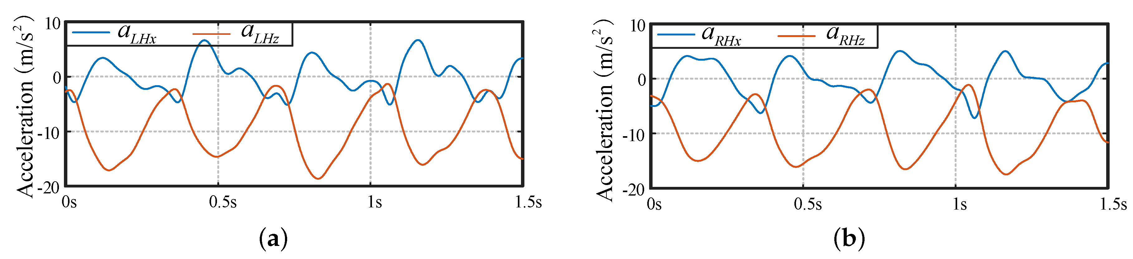
Figure 8 shows the acceleration on hip and knee joints in the sagittal plane. Both $a_{LHx}$ and $a_{RHx}$ vary around the zero axis in the range of (−5 m/s${}^2$, 5 m/s${}^2$), and $a_{LHz}$ and $a_{RHz}$ have a − 9.8 m/s${}^2$ bias caused by gravity.

(3)

The Joint Kinematics Information

Figure 9 shows the displacement of hydraulic cylinders and the angles of the hip and knee joints of the exoskeleton robot. The stroke range of the linear displacement sensor is (0 mm, 73 mm), corresponding to the knee joint angle range of ($0^{\circ }$, ${135}^{\circ }$), and that of the hip joint of ($-{15}^{\circ }$, ${150}^{\circ }$). During running in place, the hip and knee joint angles varied from ${38}^{\circ }$ to ${65}^{\circ }$ and from ${60}^{\circ }$ to ${100}^{\circ }$, respectively. The four joints did not reach the stroke limit. The lengths of the thighs and shanks of the exoskeleton were manually adjusted to be slightly larger than those of the user. This helps to avoid a dead point when the knee joint approaches $0^{\circ }$. Doing this does not affect the motion mapping.

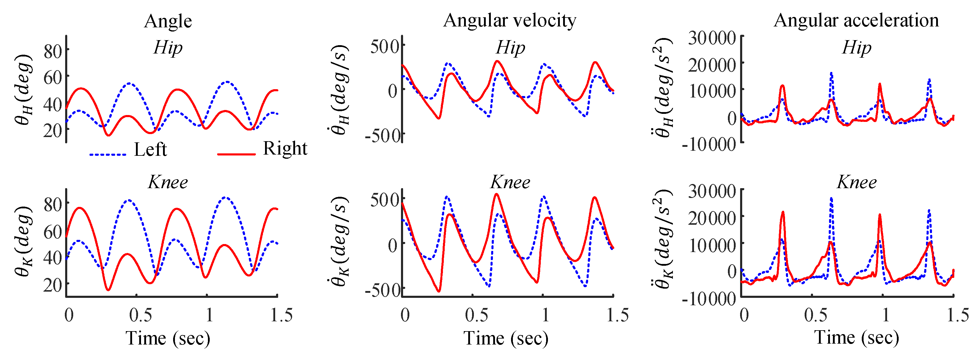
Figure 10 shows the motion information of the human body. It can be seen that the joint angular velocity is relatively smooth, but sharp variations appear in the angular acceleration which are caused by the touchdown impact.

(4)

The Foot Contact Forces

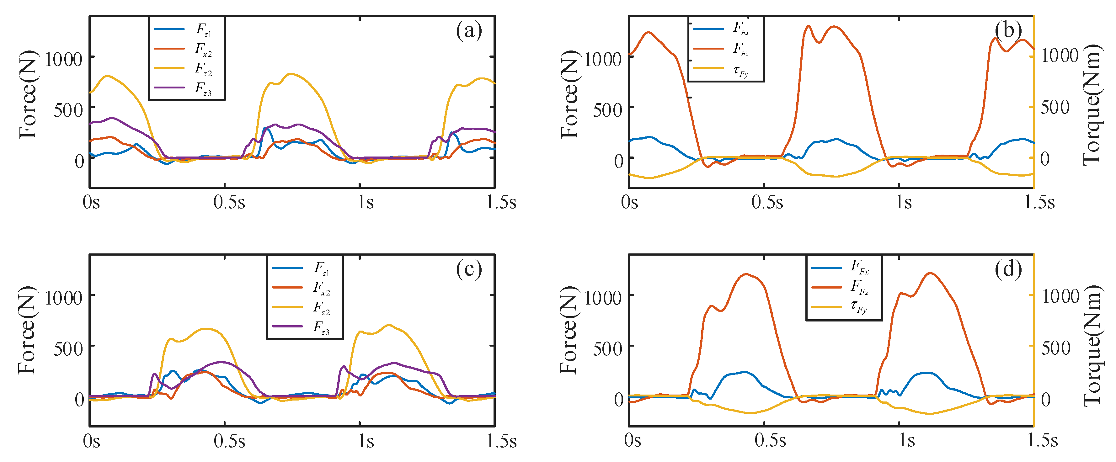
The signals from the sensor and the resultant force are shown in Figure 11. During running in place, the toe touches the ground first, so a force ($F_{z3}$) below the toe is generated. The appearance of $F_{z1}$ from the heel indicates that the entire foot is on the ground. The following is the push-off process. The resultant force in the vertical direction is significantly higher than the user ’s gravity, pushing the body to accelerate upwards and leap. Until the overall toe force drops to zero, the foot leaves the ground and switches to the swing phase. At this stage, FCF should be zero, but since the power system of the exoskeleton is not switched on, the gravity of the exoskeleton leg poses a negative vertical force on the human foot. This demonstrates that the force measurement shoe is adaptable to different foot contact states. It can measure the human FCF in both the stance and the swing phases.

(5)

JMT estimation

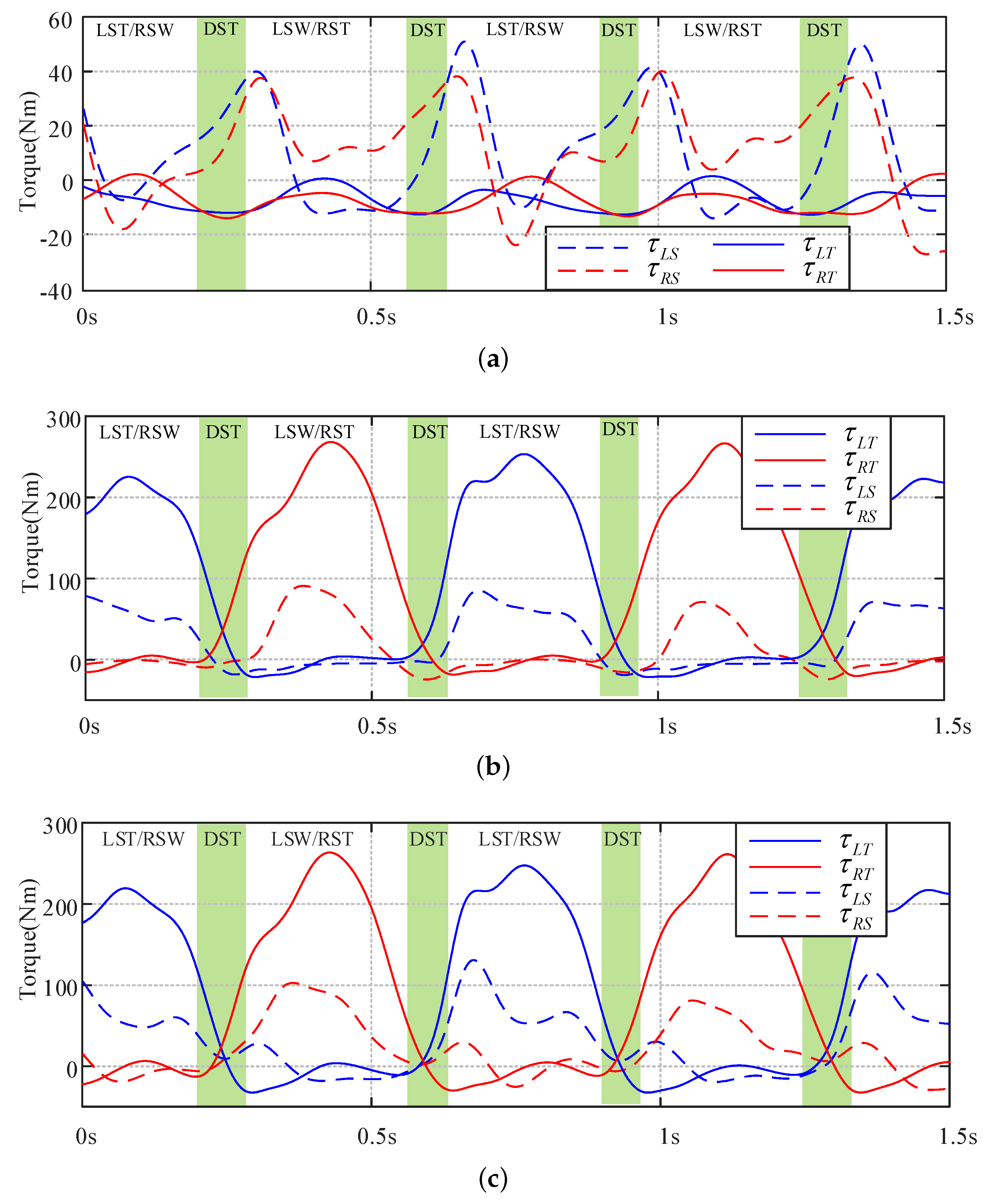
After all required parameters and variables for solving the human inverse dynamics equation were obtained, the mass-induced torques at the hip and knee joints ${\tau }_{T1}$ and ${\tau }_{S1}$ were derived via Equation (7), as shown in Figure 12a. The FCF-induced torques (${\tau }_{T2}$ and ${\tau }_{S2}$) were derived via Equation (8), as shown in Figure 12b. The resultant JMT (${\tau }_T$) was calculated via Equation (9), as shown in Figure 12c.

In Figure 12c, LST means the left leg is in stance phase, LSW means the left leg is in swing phase, R means the right leg, and DST means both the left and the right legs are in the stance phase. As shown in Figure 12a, the left hip torque drops to −7.3 Nm in the stance phase and rises up to about 40 Nm just after the DST. It again drops to −12.3 Nm in the middle of swing phase, and rises up to about 51 Nm before the left leg enters the stance phase. The trend of the right hip torque is similar to the left one. The knee torques are significantly smaller than the hip torque, because the knee only drives the shank and foot, but the hip takes the entire mass of the leg. The amplitudes of mass-induced JMT show no significant difference between the swing and the stance phase.

The FCF-induced torque shown in Figure 12b is significantly larger than the mass-induced torque. All FCF-induced JMT in swing phase are very small. However, in the stance phase, the peak of the hip torques reach up to 90 Nm, while the peak of the knee torques rise up to about 270 Nm. Unlike the mass-induced torques, the knee torques are larger than the hip torques. Most of the time, FCF-induced hip and knee torques during running in place are positive because the knees usually bend during stance phase and the upper body leans forward. The total torques are combinations of the mass-induced torques and the FCF-induced torques. Their amplitudes and curves are close to the FCF-induced torques, which indicates that the FCF-induced torques are the major parts. The trend of the right leg is similar to the left leg, but some local differences still exist due to the asymmetric nature of the two legs.

From the results, we can declare that the proposed method successfully acquired the joint torque of the human body without any auxiliary devices. The integrated sensor system ensures its portability. Besides, there is no need to mount sensors on the human body. This makes it easier to wear and take off. The newly designed IDA process is also beneficial to the accuracy of torque estimation. The mass-induced joint torque is far smaller than the FCF-induced one. According to Equation (8), FCF and the joint angles are major factors that influence the FCF-induced torque. Since the FCF is directly measured by force sensors, and the joint angles are derived from the signals of the displacement sensors, errors caused by the differentiation and inaccuracy of the human model do not influence the major part of the final results. As shown in Figure 11, even though large impacts existed in the angular accelerations of the hip and knee joints, they did not cause noticeable mutations in the total torque curves. The torque curves were smooth and continuous, which allows an exoskeleton robot to provide compliant man–machine coordination, because whatever the foot contact status changes into, no switching of dynamic equations is required; thus, there is no sudden change in the output.

3.2. Comparison Experiments

We carried out comparison experiments with an independent motion analysis system (MAS) developed by Motion Analysis Corporation (Santa Rosa, CA, USA) to verify the overall accuracy and adaptability of the proposed method with different users in different motion. Five subjects were employed to wear the APAL exoskeleton, and 22 markers were attached to each subject. The subject performed squatting, running in place and jumping motions on the force plates of the MAS 30 times each. The hip, knee, and ankle joint torques of the human body were calculated by both the exoskeleton and the MAS independently. The performance of the proposed method was quantitatively evaluated by inspecting the root-mean-square error (RMSE) and the correlation coefficient (CC) of the torque from the exoskeleton and the MAS.

Note that differences existed in the output JMT between the exoskeleton and the MAS due to the fact that the weight of the exoskeleton influences the actual JMT of the human body, but the MAS does not incorporate the existence and influence of the exoskeleton. The influence should be eliminated to make the outputs from the MAS and the exoskeleton comparable. The force (${\mathbf{F}}_{Exo}$) is caused by the weight that the exoskeleton exerts onto the human trunk and transfers to the force plate of the MAS. We calculated this force using the inverse dynamics of the exoskeleton and subtracted it from the force plates’ signals to avoid influencing the output of the MAS. We exerted a virtual inverted ${\mathbf{F}}_{Exo}$ to the human trunk while calculating the JMT with our method. By doing this, the theoretical output of the two systems should be the same.

Figure 13 demonstrates the difference in joint torques of subject 1 calculated by the exoskeleton and the MAS. Three kinds of motion were measured. The gait cycles of squatting and jumping motions start when the trunk begins moving downward, and end at stand straight. The gait cycles of each leg during running in place start and end at stance-to-swing shifting. The average torque curve of each joint under the three different types of motion appear to have preferable accordance. The error bands of the knee and ankle torques from the exoskeleton are slightly smaller than the MAS, which means our method obtains more stable torque values for the knee and ankle than the MAS.

According to the RMES shown in

Table 2. Root-mean-square error (RMSE) of the torque from the exoskeleton and the motion analysis system (MAS).

		Squat			Run			Jump
		Hip	Knee	Ankle	Hip	Knee	Ankle	Hip	Knee	Ankle
S1	Left	25.2	8	1.4	14.4	12.3	2.5	29.4	14.8	4.4
	Right	22.5	7.8	1.1	15	6.9	2.2	30.1	15.8	5.5
S2	Left	6.8	5.8	1.1	21.1	6.9	2.3	15.5	9	2.1
	Right	7.1	6.1	1.2	24.9	6.9	2.7	14.2	9.4	2.2
S3	Left	7.3	2.9	1	10.7	6.1	1.2	6.8	6.2	1.5
	Right	10.3	3.2	0.3	16.5	3.7	1.3	7.3	6.2	1.6
S4	Left	12	2.5	0.7	14.3	11.9	3.9	12.6	5.2	1.3
	Right	14.8	2.8	1.9	13.3	10.5	5.3	14	5	3.7
S5	Left	16.1	2.3	0.8	6.3	5.8	5	16.8	6.8	2.4
	Right	18	3.6	1.5	5.3	3.2	5.5	16.8	5.4	4.1
Mean SD		14	4.5	1.1	14.2	7.4	3.2	16.4	8.4	2.9
		6.5	2.2	0.5	6	3.2	1.6	7.9	3.9	1.4

, we can see three phenomenon: (1) The error of ankle torque is very small for all subjects in each motion, which means the FCF from contact force measurement shoe is quite accurate, and the neglect of inertial torque caused by ankle movement did not lead to a large error of ankle joints; (2) in general, the further the joint is from the foot plate, the larger the error appears, because of the cumulative error of the limb length and joint angle. The RMSE of the hip joint is larger than that of the knee joint, even though the maximal torque of hip is smaller, as shown in Figure 13, and the RMSE of the knee is also larger than that of the ankle. (3) Comparing the individual RMSE to the average RMSE of the five subjects, differences between individuals truly exist but are not significant—these differences are mainly caused by individual parameter error. If a more accurate result is required, individual parameters, such as limb length, mass, inertial, and the mass center of each limb, should be further investigated, like B. Hwang et al. did in Ref. [28].

Table 3. Correlation coefficient of the torque from the exoskeleton and the MAS.

		Squat			Run			Jump
		Hip	Knee	Ankle	Hip	Knee	Ankle	Hip	Knee	Ankle
S1	Left	0.875	0.985	0.990	0.928	0.948	0.998	0.812	0.958	0.963
	Right	0.877	0.988	0.993	0.850	0.989	0.998	0.832	0.954	0.955
S2	Left	0.700	0.983	0.953	0.903	0.993	0.994	0.629	0.974	0.979
	Right	0.891	0.976	0.965	0.862	0.993	0.991	0.732	0.962	0.982
S3	Left	0.932	0.995	0.982	0.874	0.978	0.999	0.896	0.978	0.986
	Right	0.867	0.996	0.999	0.707	0.995	0.999	0.922	0.982	0.990
S4	Left	0.908	0.998	0.996	0.705	0.882	0.993	0.904	0.988	0.995
	Right	0.886	0.997	0.979	0.710	0.918	0.989	0.851	0.985	0.963
S5	Left	0.836	0.998	0.997	0.839	0.988	0.99	0.783	0.973	0.985
	Right	0.704	0.997	0.993	0.745	0.996	0.991	0.743	0.988	0.972
Mean SD		0.848	0.991	0.985	0.812	0.968	0.994	0.810	0.974	0.977
		0.081	0.008	0.019	0.082	0.040	0.004	0.091	0.012	0.013

shows the CC of the torque from the exoskeleton and the MAS. The CC reveals the similarity between the torque curves. There are several phenomenon: (1) Most average CC values are larger than 0.81. The average CC values of the knees and ankles are all larger than 0.96; only the hip joint during running in place drops to 0.81. This means that the overall similarity is not too bad. (2) The standard deviation (SD) of CC of the five subjects are smaller than 0.091; in particular, those of knee and ankle joints are smaller than 0.04. This indicates that the proposed method is individual independent. (3) The lack of significant differences between the trends of each joint during different motions means that the proposed method is valid for relatively complex motion. (4) The data of the hip joint was shown to be more volatile than the knee and ankle joints, but no subversive data appeared.

4. Conclusions

This paper proposed a novel human lower limb JMT estimation solution based on an IDA. The method has two main parts: the sensing system and the inverse dynamic approach. The embedded sensing system makes the exoskeleton easier to use than the popular EMG based devices. All subjects only need several seconds to put on the exoskeleton and input his/her weight and height; no electrodes or other sensors are required to be fixed onto the human body. Comparison experiments show similar outputs to an independent motion analysis system. According to the quantitative analysis of the two outputs from the exoskeleton and the MAS, the result shows accordance accuracy with different subjects in different motions, which indicates the individual independent character of the proposed method and its adaptability to a variety of motion patterns. Benefitting from the measurement of the FCF, the shortening of the kinematic chain helps to reduce the computational complexity through the strategy of factorizing the JMT into mass-induced one, and FCF-induced one cancels the necessity of a finite-state-machine and ensures the continuity of the JMT output.

This study only investigated motion in the sagittal plane. In the future, we want to explore this method to random motion in $3D$ space. In that time, the side-sway and supination/pronation of the hip joints should be measured, and the $6D$ force/torque of the feet should be measured. The IDA equation should take the coronal and frontal motion into account. In addition, automatic identification of the individual parameters may help to further improve the accuracy.

References

- Kazerooni, H.; Racine, J.L.; Huang, L.; Steger, R. On the control of the berkeley lower extremity exoskeleton (BLEEX). In Proceedings of the 2005 IEEE International Conference on Robotics and Automation, Barcelona, Spain, 18–22 April 2005; pp. 4353–4360. [Google Scholar]
- Hiroaki, K.; Yoshiyuki, S. Power assist method based on Phase Sequence and muscle force condition for HAL. Adv. Robot. 2005, 19, 717–734. [Google Scholar]
- Collins, S.H.; Wiggin, M.B.; Sawicki, G.S. Reducing the energy cost of human walking using an unpowered exoskeleton. Nature 2015, 522, 212–215. [Google Scholar] [CrossRef] [PubMed] [Green Version]
- Asbeck, A.T.; Rossi, S.M.M.D.; Holt, K.G.; Walsh, C.J. A biologically inspired soft exosuit for walking assistance. Int. J. Robot. Res. 2015, 34, 744–762. [Google Scholar] [CrossRef]
- Khan, A.M.; Yun, D.W.; Zuhaib, K.M.; Iqbal, J.; Yan, R.J.; Khan, F.; Han, C. Estimation of Desired Motion Intention and compliance control for upper limb assist exoskeleton. Int. J. Control Autom. Syst. 2017, 15, 802–814. [Google Scholar] [CrossRef]
- Chen, C.; Wu, X.; Liu, D.X.; Feng, W.; Wang, C. Design and Voluntary Motion Intention Estimation of a Novel Wearable Full-Body Flexible Exoskeleton Robot. Mob. Inf. Syst. 2017, 2017, 1–11. [Google Scholar] [CrossRef] [Green Version]
- Kenta, S.; Gouji, M.; Hiroaki, K.; Yasuhisa, H.; Yoshiyuki, S. Intention-based walking support for paraplegia patients with Robot Suit HAL. Adv. Robot. 2007, 21, 1441–1469. [Google Scholar]
- Yang, C.; Wang, X.; Li, Z.; Li, Y.; Su, C.Y. Teleoperation Control Based on Combination of Wave Variable and Neural Networks. IEEE Trans. Syst. Man Cybern. Syst. 2017, 47, 2125–2136. [Google Scholar] [CrossRef] [Green Version]
- Zhijun, L.I.; Zhao, T.; Chen, F.; Hu, Y.; Su, C.Y.; Fukuda, T. Reinforcement Learning of Manipulation and Grasping using Dynamical Movement Primitives for a Humanoid-like Mobile Manipulator. IEEE/ASME Trans. Mechatron. 2017. [Google Scholar] [CrossRef]
- Sankai, Y. HAL: Hybrid Assistive Limb Based on Cybernics. In Proceedings of the Isrr 2007 Robotics Research—The International Symposium, Hiroshima, Japan, 26–29 November 2007; pp. 25–34. [Google Scholar]
- Lloyd, D.G.; Besier, T.F. An EMG-driven musculoskeletal model to estimate muscle forces and knee joint moments in vivo. J. Biomech. 2003, 36, 765–776. [Google Scholar] [CrossRef] [Green Version]
- Krasin, V.; Gandhi, V.; Yang, Z.; Karamanoglu, M. EMG based elbow joint powered exoskeleton for biceps brachii strength augmentation. In Proceedings of the International Joint Conference on Neural Networks, Killarney, Ireland, 12–17 July 2015; pp. 1–6. [Google Scholar]
- Peternel, L.; Noda, T.; Petrič, T.; Ude, A.; Morimoto, J.; Babič, J. Adaptive Control of Exoskeleton Robots for Periodic Assistive Behaviours Based on EMG Feedback Minimisation. PLoS ONE 2016, 11, e0148942. [Google Scholar] [CrossRef] [PubMed] [Green Version]
- Cristian, C.; Marco, C.; Giuseppe, C. Design and numerical characterization of a new leg exoskeleton for motion assistance. Robotica 2015, 33, 1147–1162. [Google Scholar]
- Spring, A.N.; Kofman, J.; Lemaire, E.D. Design and evaluation of an orthotic knee-extension assist. IEEE Trans. Neural Syst. Rehabil. Eng. 2012, 20, 678–687. [Google Scholar] [CrossRef] [PubMed]
- Buchanan, T.S.; Lloyd, D.G.; Manal, K.; Besier, T.F. Estimation of muscle forces and joint moments using a forward-inverse dynamics model. Med. Sci. Sports Exerc. 2005, 37, 1911–1916. [Google Scholar] [CrossRef] [PubMed]
- Yang, C.; Zeng, C.; Liang, P.; Li, Z.; Li, R.; Su, C.Y. Interface Design of a Physical Human-Robot Interaction System for Human Impedance Adaptive Skill Transfer. IEEE Trans. Autom. Sci. Eng. 2017, 1–12. [Google Scholar] [CrossRef]
- Tucker, M.R.; Olivier, J.; Pagel, A.; Bleuler, H.; Bouri, M.; Lambercy, O.; Millán, J.R.; Riener, R.; Vallery, H.; Gassert, R. Control strategies for active lower extremity prosthetics and orthotics: A review. J. Neuroeng. Rehabil. 2015, 12. [Google Scholar] [CrossRef] [PubMed] [Green Version]
- Pal, A.R.; Pratihar, D.K. Estimation of Joint Torque and Power Consumption During Sit-to-Stand Motion of Human-being Using a Genetic Algorithm. Procedia Comput. Sci. 2016, 96, 1497–1506. [Google Scholar] [CrossRef]
- Camomilla, V.; Cereatti, A.; Cutti, A.G.; Fantozzi, S.; Stagni, R.; Vannozzi, G. Methodological factors affecting joint moments estimation in clinical gait analysis: A systematic review. Biomed. Eng. Online 2017, 16, 106. [Google Scholar] [CrossRef] [PubMed]
- Shull, P.B.; Jirattigalachote, W.; Hunt, M.A.; Cutkosky, M.R.; Delp, S.L. Quantified self and human movement: A review on the clinical impact of wearable sensing and feedback for gait analysis and intervention. Gait Posture 2014, 40, 11–19. [Google Scholar] [CrossRef] [PubMed]
- Abdul, R.A.H.; Aladin, Z.; Begg, R.K.; Yufridin, W. Foot Plantar Pressure Measurement System: A Review. Sensors 2012, 12, 9884–9912. [Google Scholar] [CrossRef] [PubMed] [Green Version]
- Kim, S.; Ro, K.; Bae, J. Real-time estimation of individual muscular forces of the lower limb using wearable sensors. In Proceedings of the 2015 IEEE International Conference on Advanced Intelligent Mechatronics (AIM), Busan, Korea, 7–11 July 2015; pp. 432–436. [Google Scholar]
- Liu, T.; Inoue, Y.; Shibata, K.; Shiojima, K. Three-dimensional lower limb kinematic and kinetic analysis based on a wireless sensor system. In Proceedings of the 2011 IEEE International Conference on Robotics and Automation (ICRA), Shanghai, China, 9–13 May 2011; pp. 842–847. [Google Scholar]
- Kazerooni, H.; Steger, R.; Huang, L. Hybrid Control of the Berkeley Lower Extremity Exoskeleton (BLEEX); Sage Publications Inc.: Thousand Oaks, CA, USA, 2006; pp. 561–573. [Google Scholar]
- Yang, C.; Zeng, C.; Fang, C.; He, W.; Li, Z. A DMPs-based Framework for Robot Learning and Generalization of Human-like Variable Impedance Skills. IEEE/ASME Trans. Mechatron. 2018, 23, 1193–1203. [Google Scholar] [CrossRef]
- Saccares, L.; Brygo, A.; Sarakoglou, I.; Tsagarakis, N.G. A novel human effort estimation method for knee assistive exoskeletons. In Proceedings of the International Conference on Rehabilitation Robotics, London, UK, 17–20 July 2017; pp. 1266–1272. [Google Scholar]
- Hwang, B.; Jeon, D. A method to accurately estimate the muscular torques of human wearing exoskeletons by torque sensors. Sensors 2015, 15, 8337–8357. [Google Scholar] [CrossRef] [PubMed]
- Hwang, B.; Jeon, D. Estimation of the user’s muscular torque for an over-ground gait rehabilitation robot using torque and insole pressure sensors. Int. J. Control Autom. Syst. 2018, 16, 1–9. [Google Scholar] [CrossRef]
- Deng, J.; Wang, P.; Li, M.; Guo, W.; Zha, F.; Wang, X. Structure design of active power-assist lower limb exoskeleton APAL robot. Adv. Mech. Eng. 2017, 9. [Google Scholar] [CrossRef]
- Leva, P.D. Adjustments to Zatsiorsky-Seluyanov’s segment inertia parameters. J. Biomech. 1996, 29, 1223–1230. [Google Scholar] [CrossRef]
- Cheng, C.K.; Chen, H.H.; Chen, C.S.; Lee, C.L.; Chen, C.Y. Segment inertial properties of Chinese adults determined from magnetic resonance imaging. Clin. Biomech. 2000, 15, 559–566. [Google Scholar] [CrossRef]
- Wang, Q.; Wang, L.; Zhu, J. Effects of toe stiffness on ankle kinetics in a robotic transtibial prosthesis during level-ground walking. Mechatronics 2014, 24, 1254–1261. [Google Scholar]