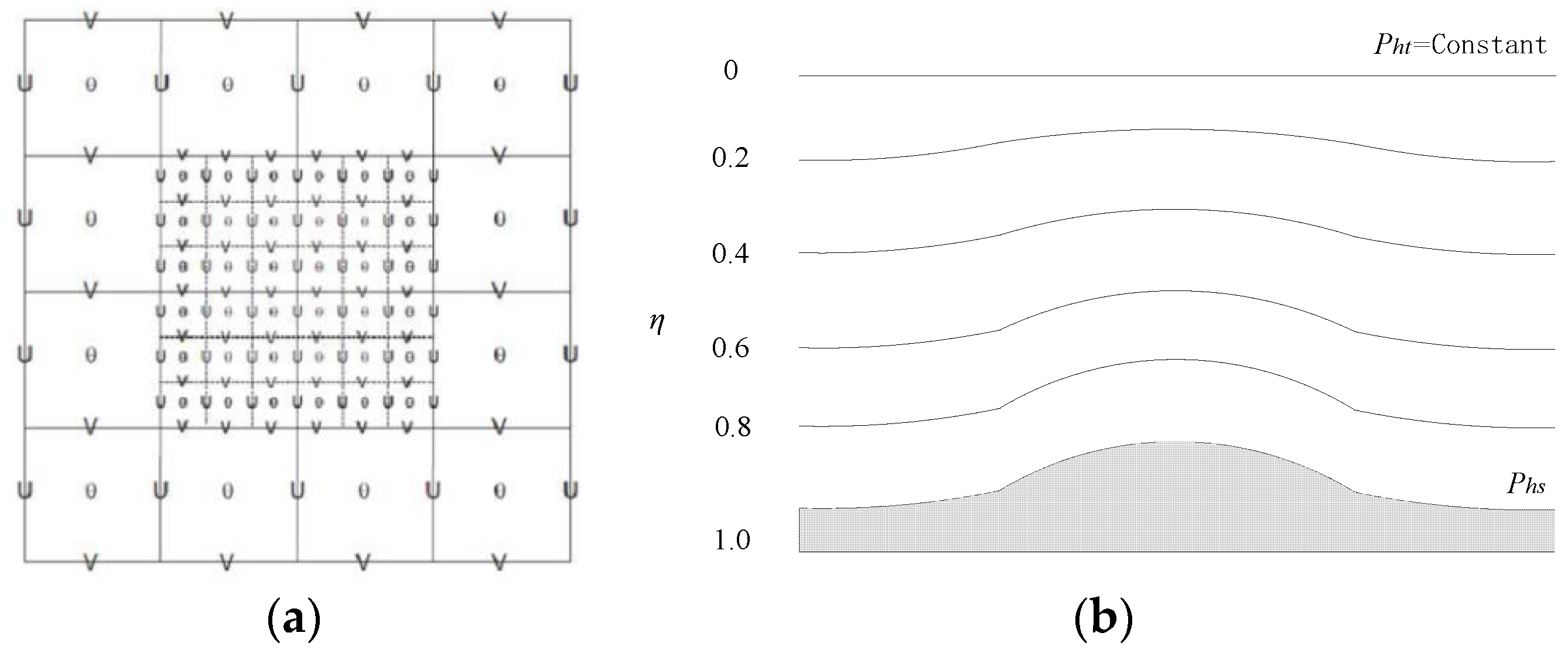
Figure 1.
Meshing of the Weather Research Forecasting (WRF) model. (a) Horizontal grids (space between coarse and thin grids is 3:1); (b) Vertical grids.
Figure 1.
Meshing of the Weather Research Forecasting (WRF) model. (a) Horizontal grids (space between coarse and thin grids is 3:1); (b) Vertical grids.
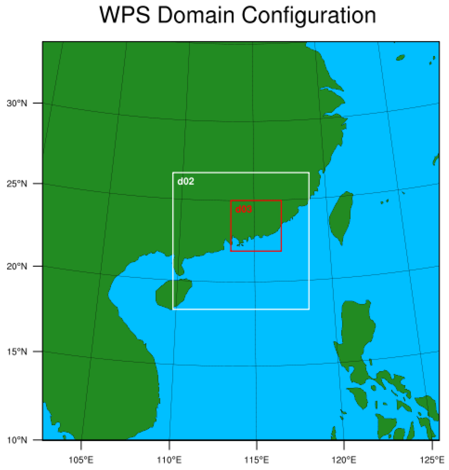
Figure 2.
Simulation domain of the Typhoon “Nuri”.
Figure 2.
Simulation domain of the Typhoon “Nuri”.
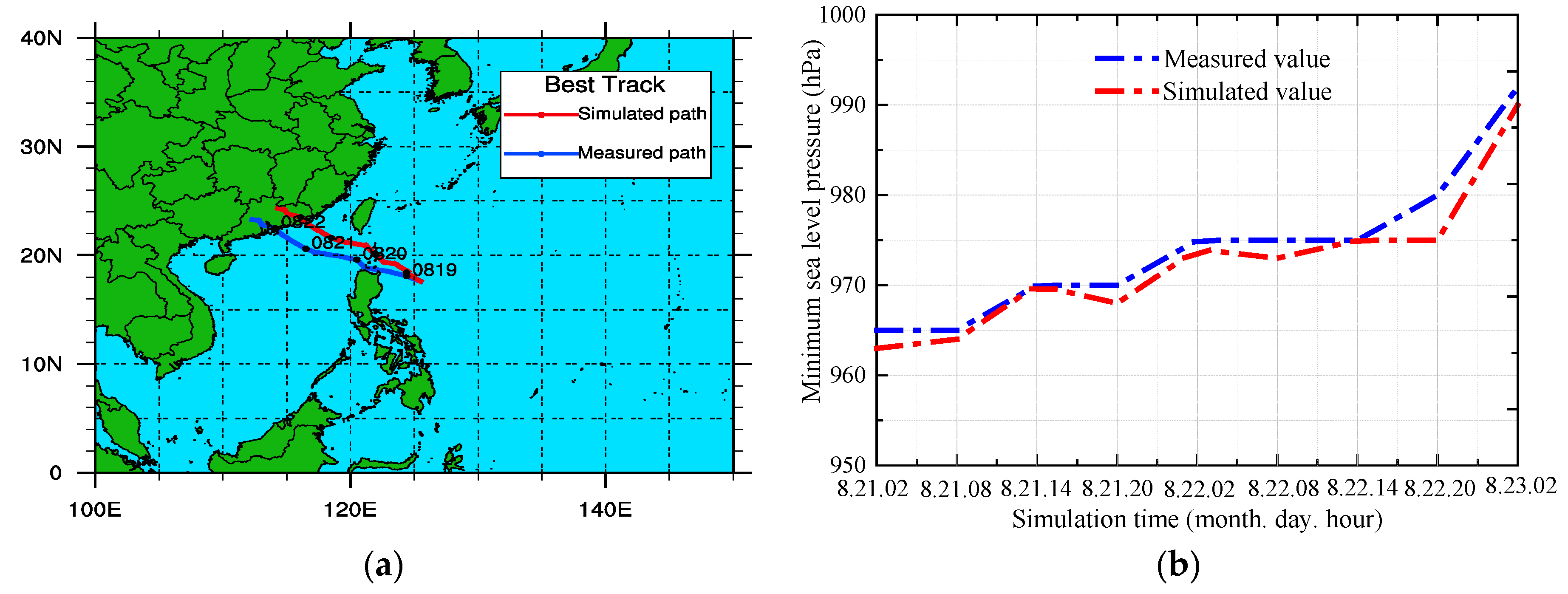
Figure 3.
Typhoon path and minimum sea level pressure throughout the simulation. (a) Typhoon path; (b) Minimum sea level pressure.
Figure 3.
Typhoon path and minimum sea level pressure throughout the simulation. (a) Typhoon path; (b) Minimum sea level pressure.
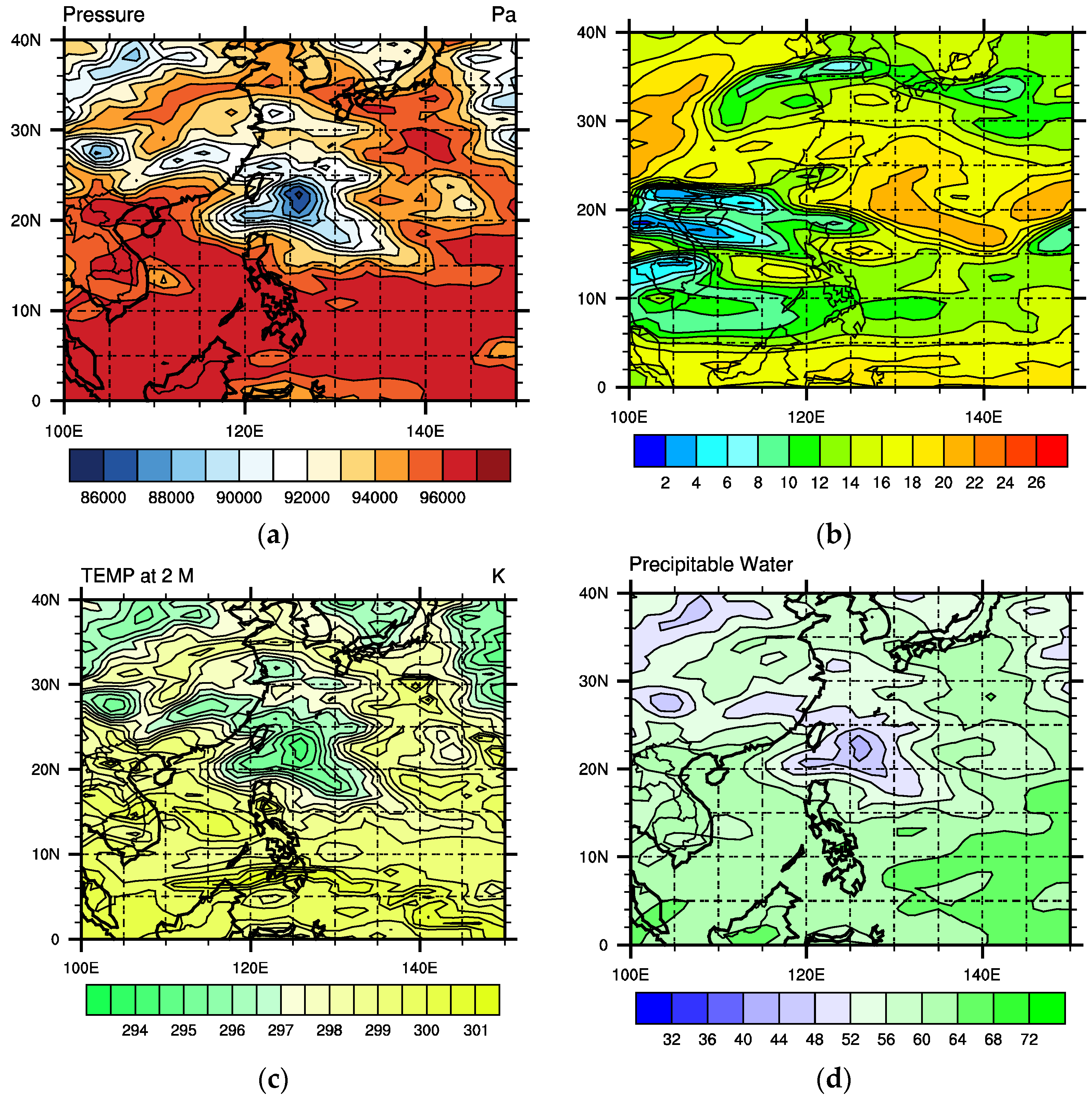
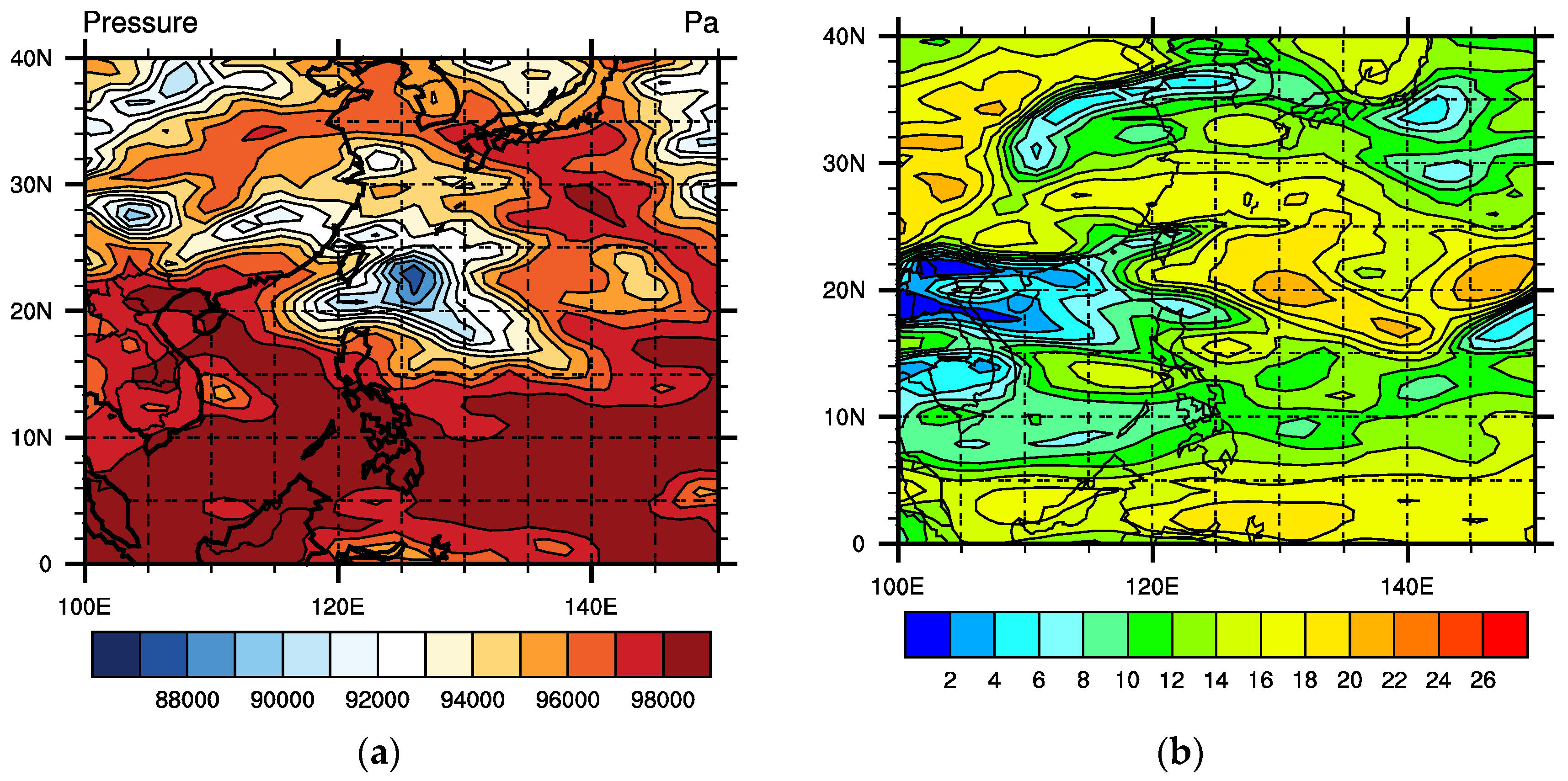
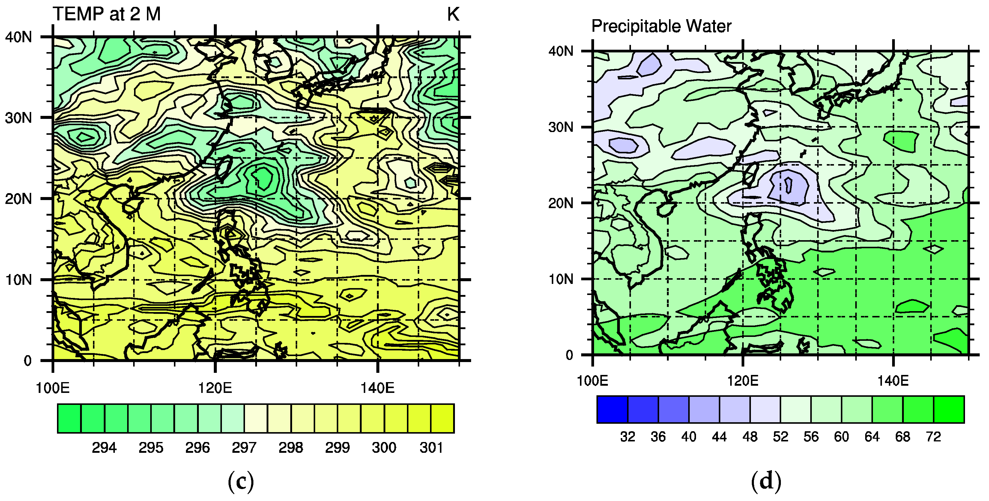
Figure 4.
Simulation results for landing of typhoon. (a) Air pressure nephogram; (b) Wind speed nephogram; (c) Temperature nephogram; (d) Rainfall nephogram.
Figure 4.
Simulation results for landing of typhoon. (a) Air pressure nephogram; (b) Wind speed nephogram; (c) Temperature nephogram; (d) Rainfall nephogram.
Figure 5.
Measured results for landing of typhoon. (a) Air pressure nephogram; (b) Wind speed nephogram; (c) Temperature nephogram; (d) Rainfall nephogram.
Figure 5.
Measured results for landing of typhoon. (a) Air pressure nephogram; (b) Wind speed nephogram; (c) Temperature nephogram; (d) Rainfall nephogram.
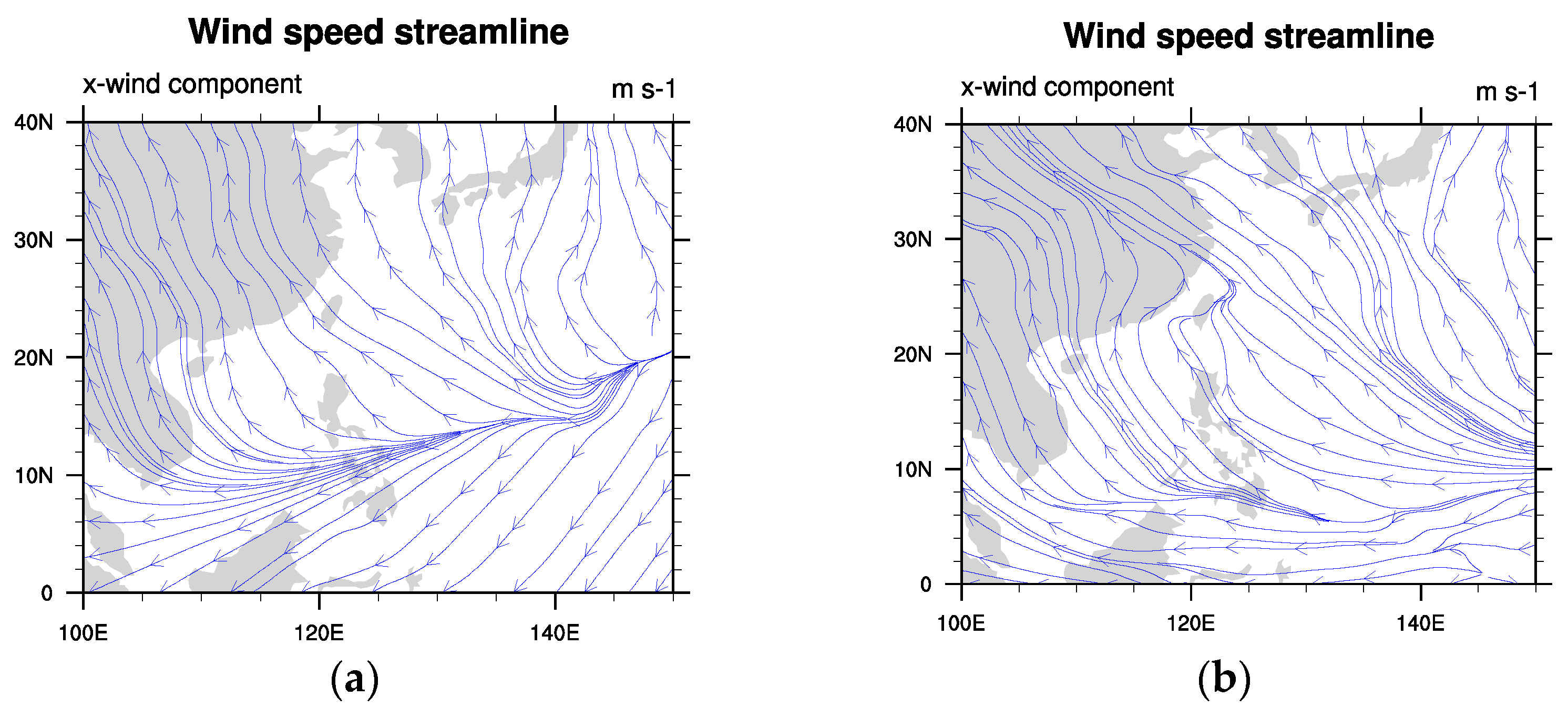
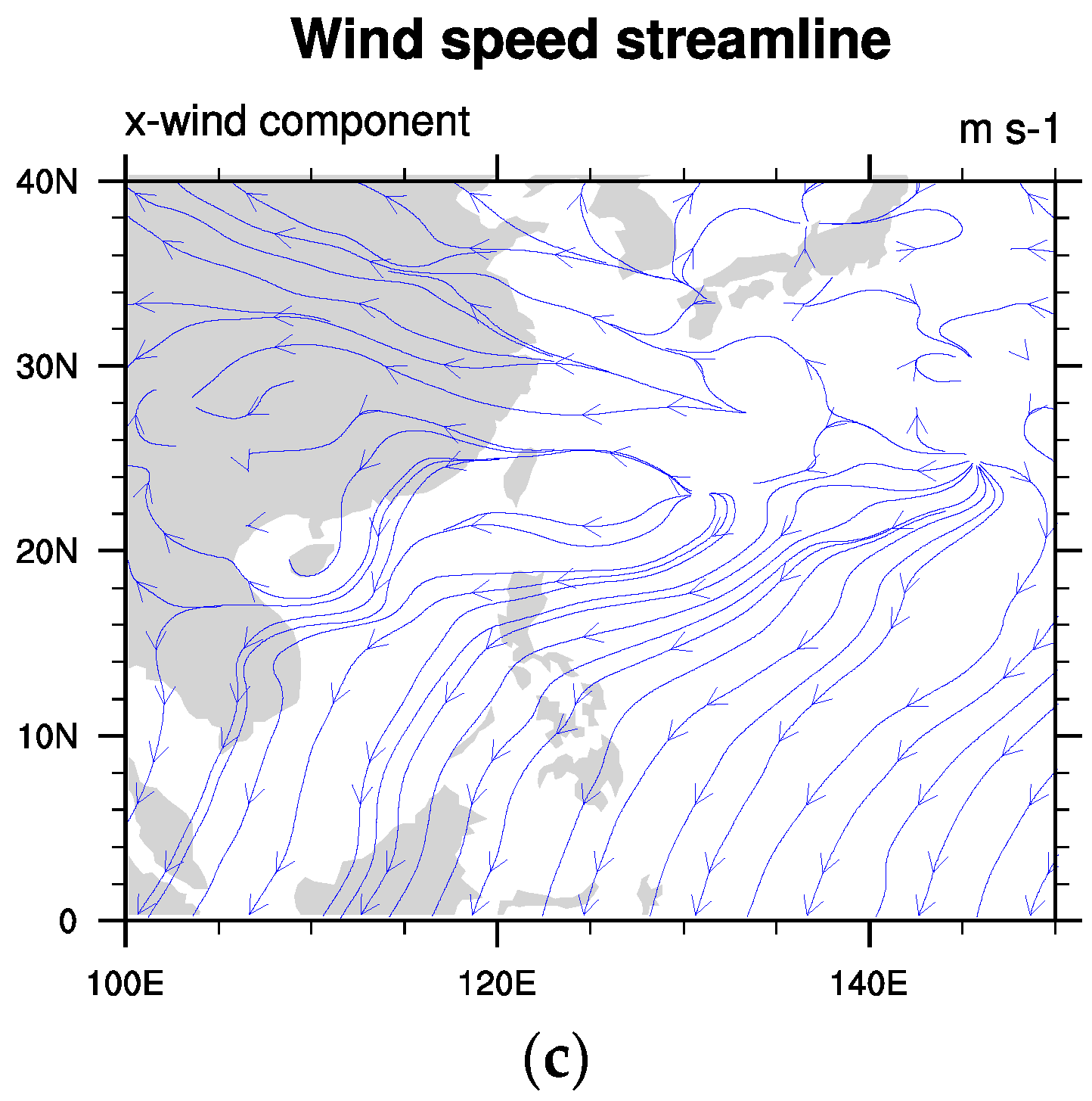
Figure 6.
Wind speed streamlines before, at, and after landing of the typhoon. (a) Before landing (14:00 on 22 August); (b) At landing (20:00 on 22 August); (c) After landing (02:00 on 23 August).
Figure 6.
Wind speed streamlines before, at, and after landing of the typhoon. (a) Before landing (14:00 on 22 August); (b) At landing (20:00 on 22 August); (c) After landing (02:00 on 23 August).
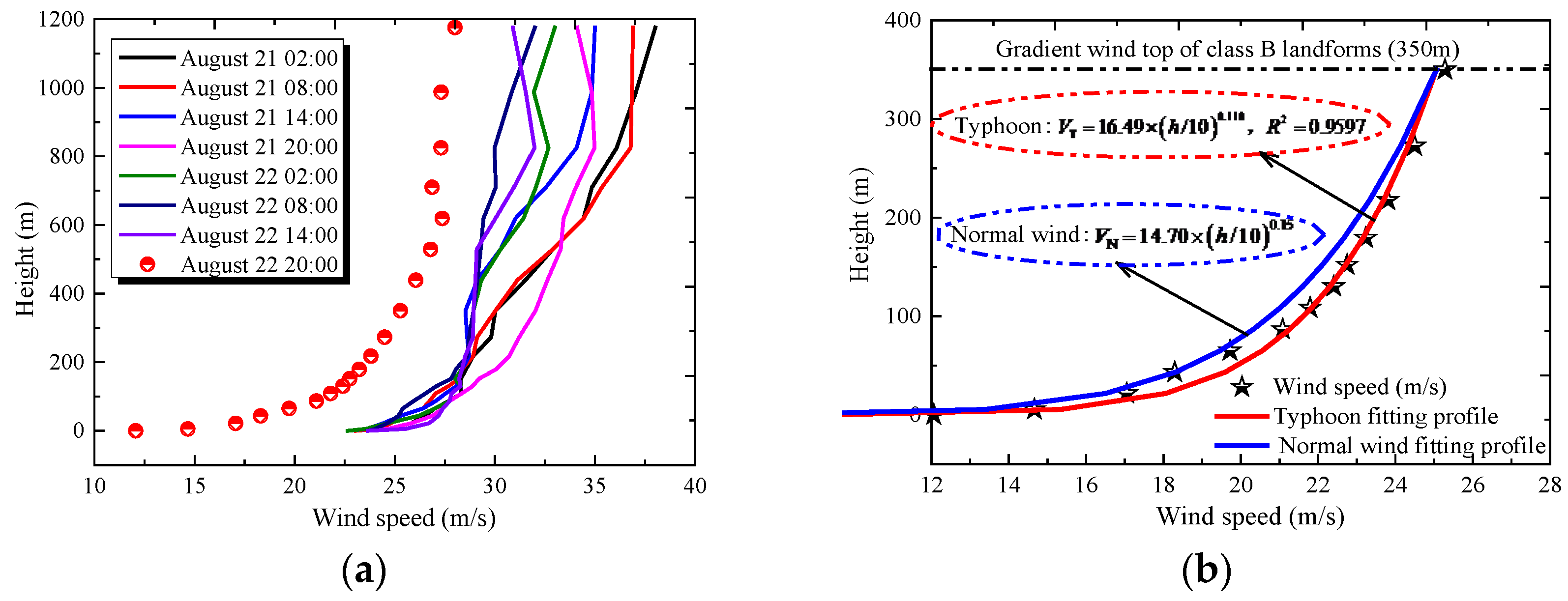
Figure 7.
Wind speed profile close to the typhoon center and near-ground wind speed and fitting curves in the center of the simulation region at different moments. (a) Wind speed profile close to the typhoon center at different moments; (b) Near-ground wind speed and fitting curves in the center of the simulation region.
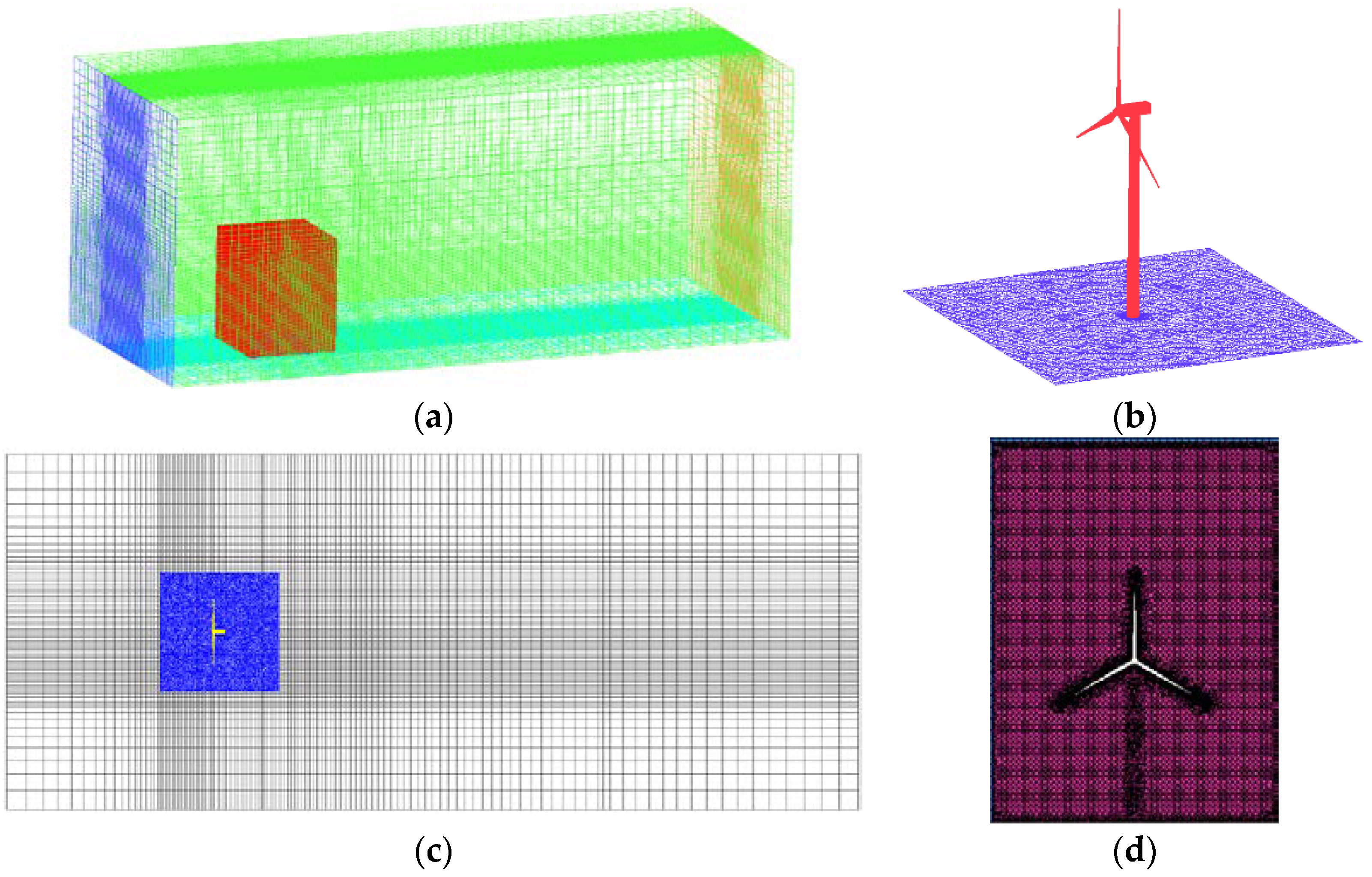
Figure 8.
Computational domain and meshing schemes. (a) Meshing of the overall computational domain; (b) Meshing of local computational domain; (c) Meshing of the x-y plane; (d) Meshing of the encrypted y-z plane.
Figure 8.
Computational domain and meshing schemes. (a) Meshing of the overall computational domain; (b) Meshing of local computational domain; (c) Meshing of the x-y plane; (d) Meshing of the encrypted y-z plane.
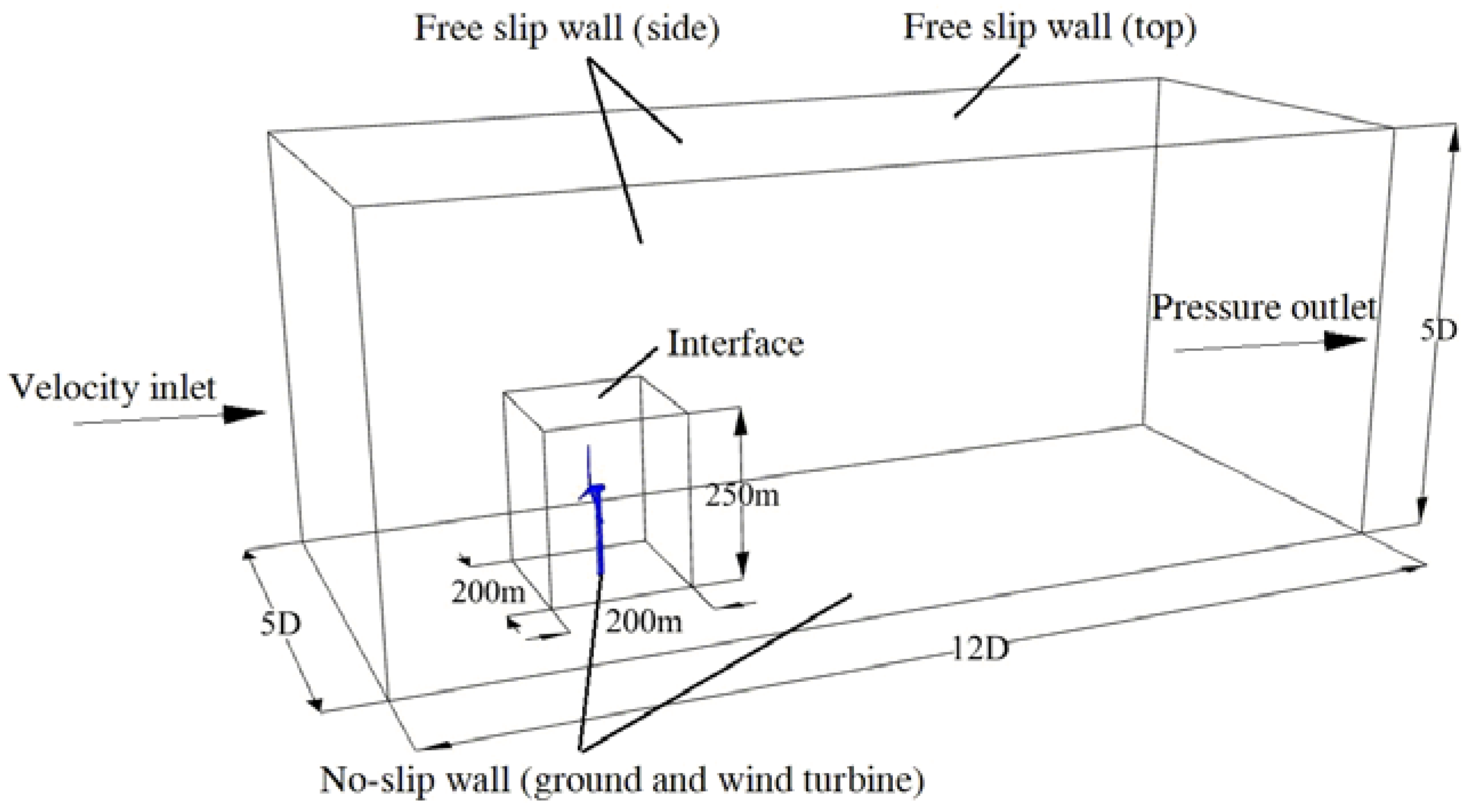
Figure 9.
Boundary conditions of the computational domain.
Figure 9.
Boundary conditions of the computational domain.
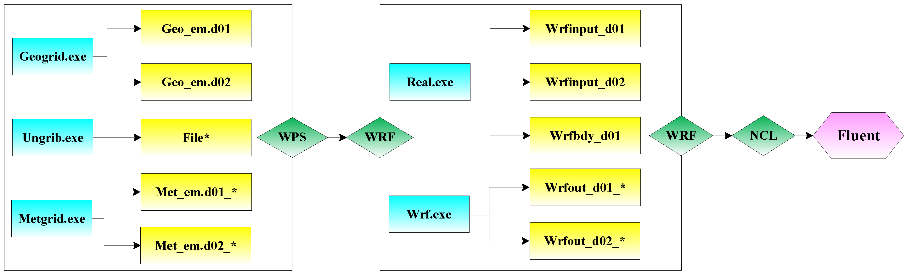
Figure 10.
Procedures of WRF-CFD (Computational Fluid Dynamics) computation and nesting.
Figure 10.
Procedures of WRF-CFD (Computational Fluid Dynamics) computation and nesting.
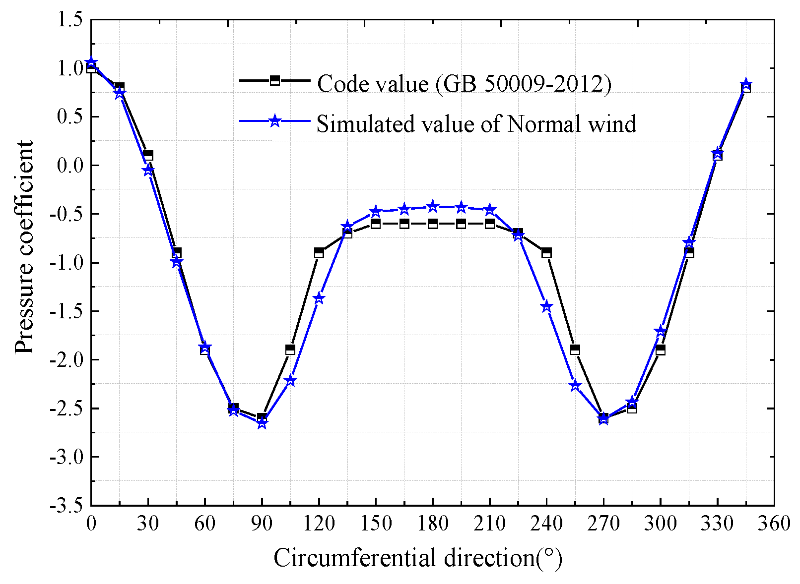
Figure 11.
Numerical simulation results under normal wind conditions versus value specified by Chinese code.
Figure 11.
Numerical simulation results under normal wind conditions versus value specified by Chinese code.
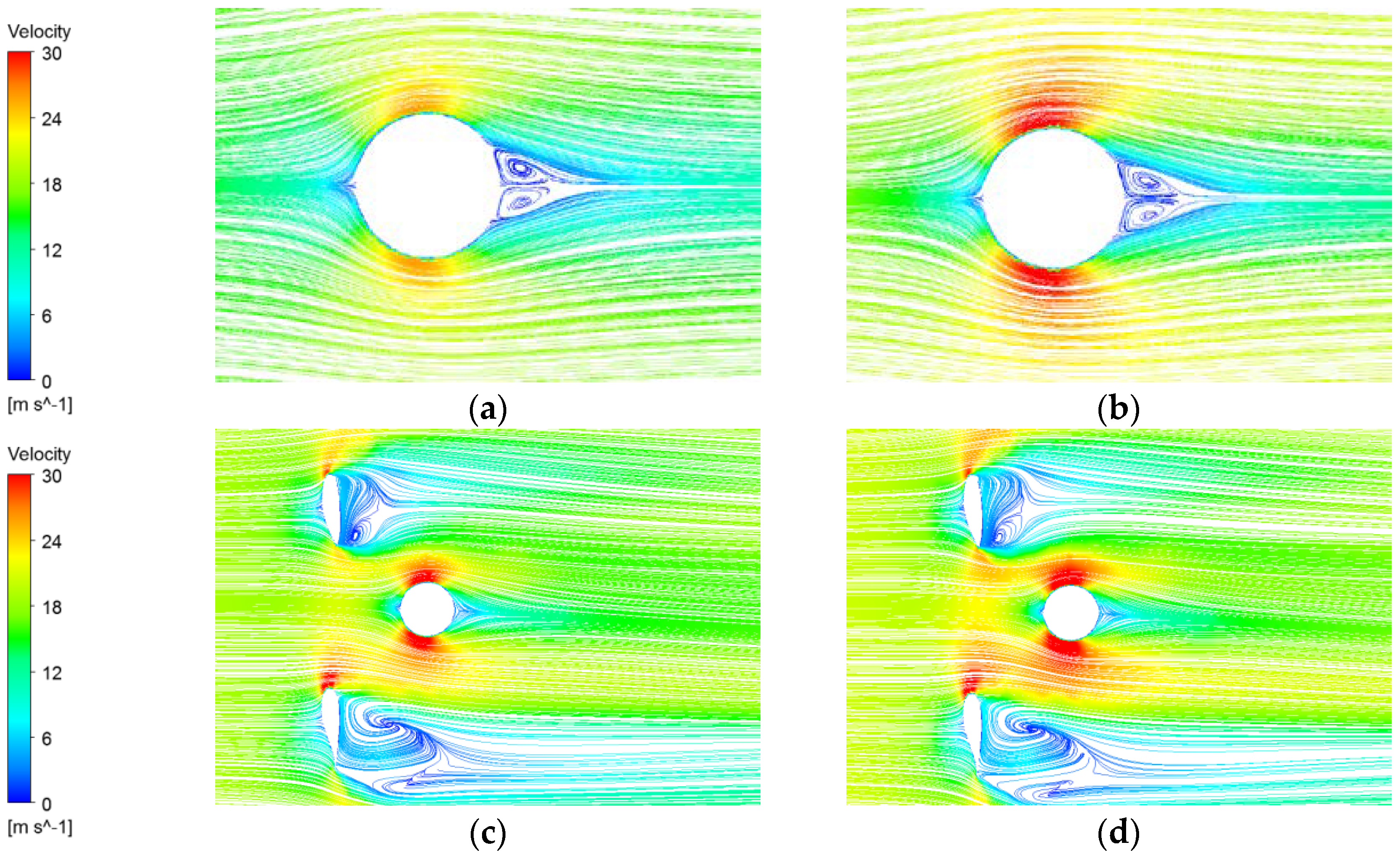
Figure 12.
Wind speed streamlines at a typical section of the tower body under normal wind and typhoon loads. (a) Normal wind (0.3H); (b) Typhoon (0.3H); (c) Normal wind (0.8H); (d) Typhoon (0.8H).
Figure 12.
Wind speed streamlines at a typical section of the tower body under normal wind and typhoon loads. (a) Normal wind (0.3H); (b) Typhoon (0.3H); (c) Normal wind (0.8H); (d) Typhoon (0.8H).
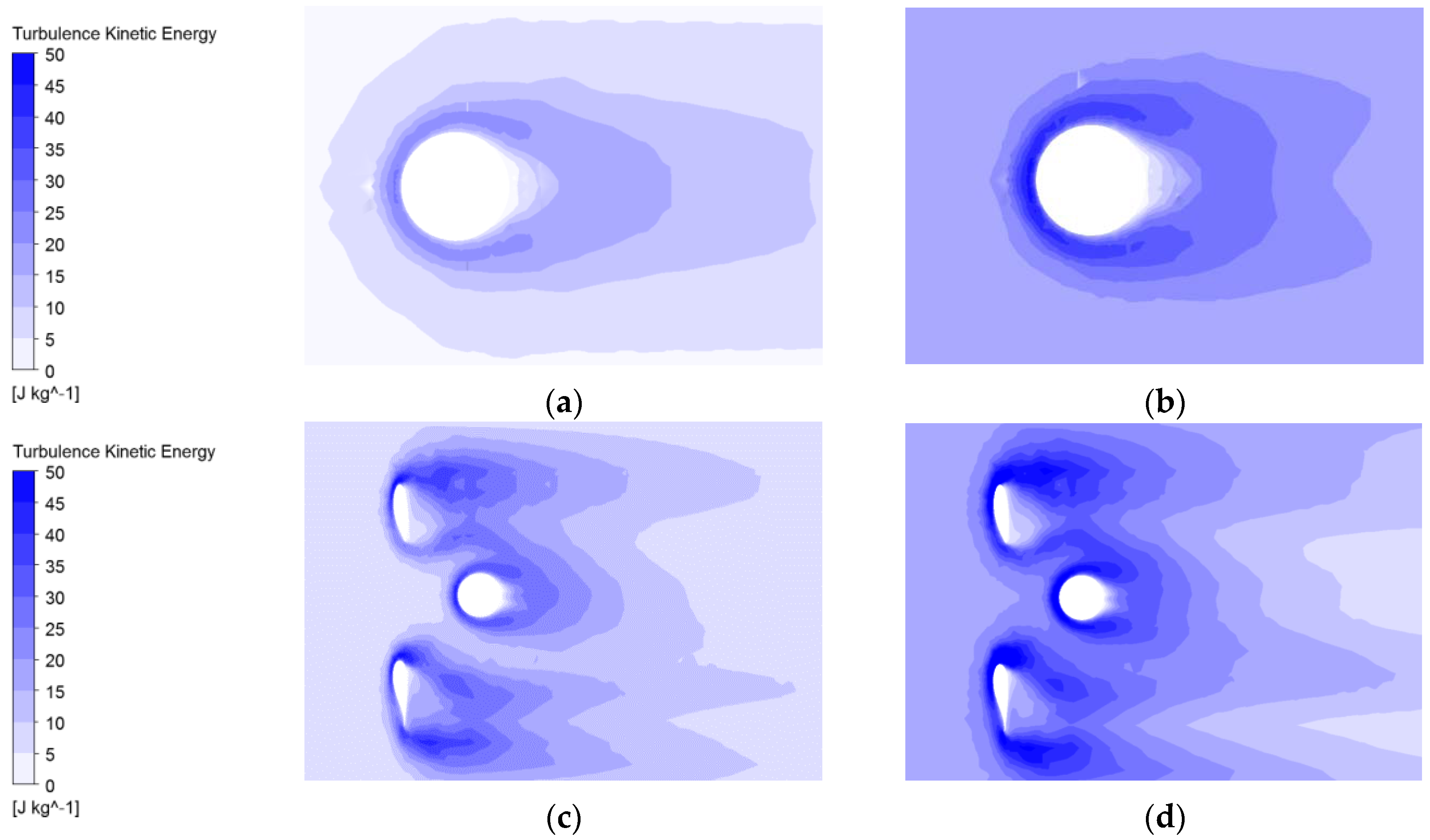
Figure 13.
Turbulence energy distribution at a typical section of the tower body under normal wind and typhoon loads. (a) Normal wind (0.3H); (b) Typhoon (0.3H); (c) Normal wind (0.8H); (d) Typhoon (0.8H).
Figure 13.
Turbulence energy distribution at a typical section of the tower body under normal wind and typhoon loads. (a) Normal wind (0.3H); (b) Typhoon (0.3H); (c) Normal wind (0.8H); (d) Typhoon (0.8H).
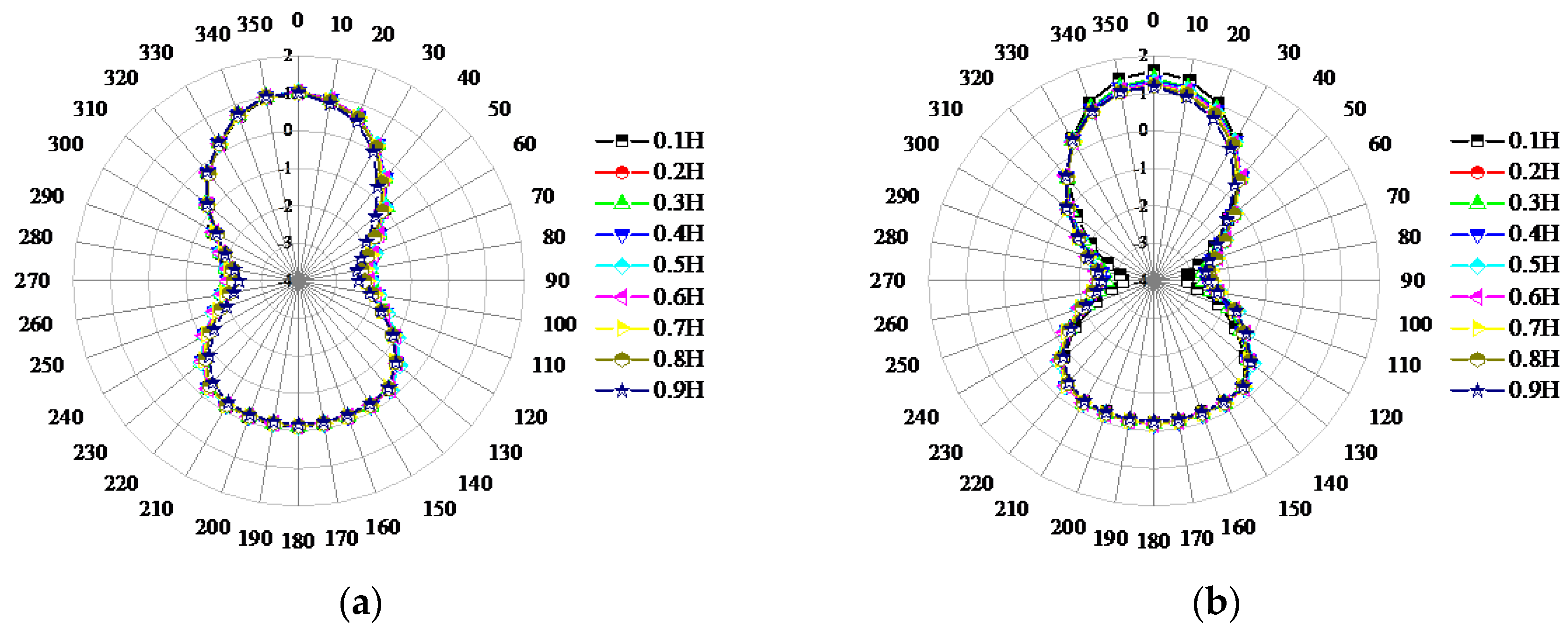
Figure 14.
Distribution curves of wind pressure coefficient on tower body under normal wind and typhoon loads. (a) Normal wind; (b) Typhoon.
Figure 14.
Distribution curves of wind pressure coefficient on tower body under normal wind and typhoon loads. (a) Normal wind; (b) Typhoon.
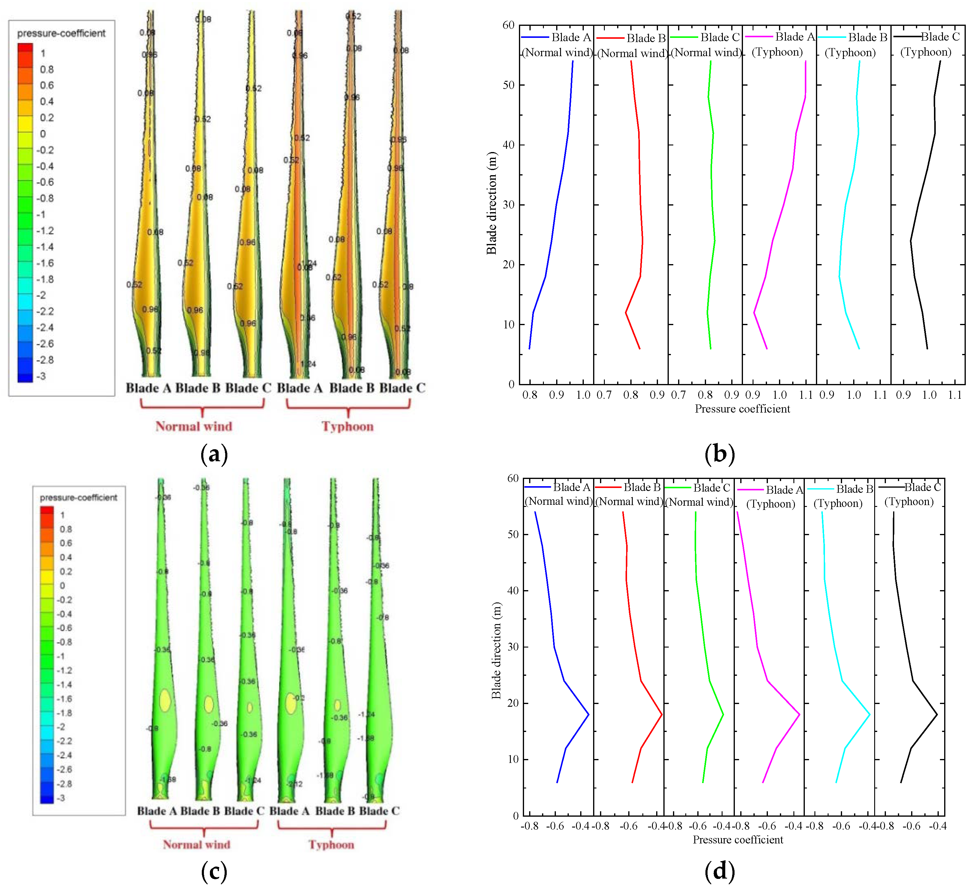
Figure 15.
Wind pressure coefficient nephograms on the windward and leeside of blades as well as the mean along the blade under normal wind and typhoon loads. (a) Wind pressure coefficient nephogram on the windward side; (b) Wind pressure coefficient curves on the windward side; (c) Wind pressure coefficient nephogram on the leeside; (d) Wind pressure coefficient curves on the leeside.
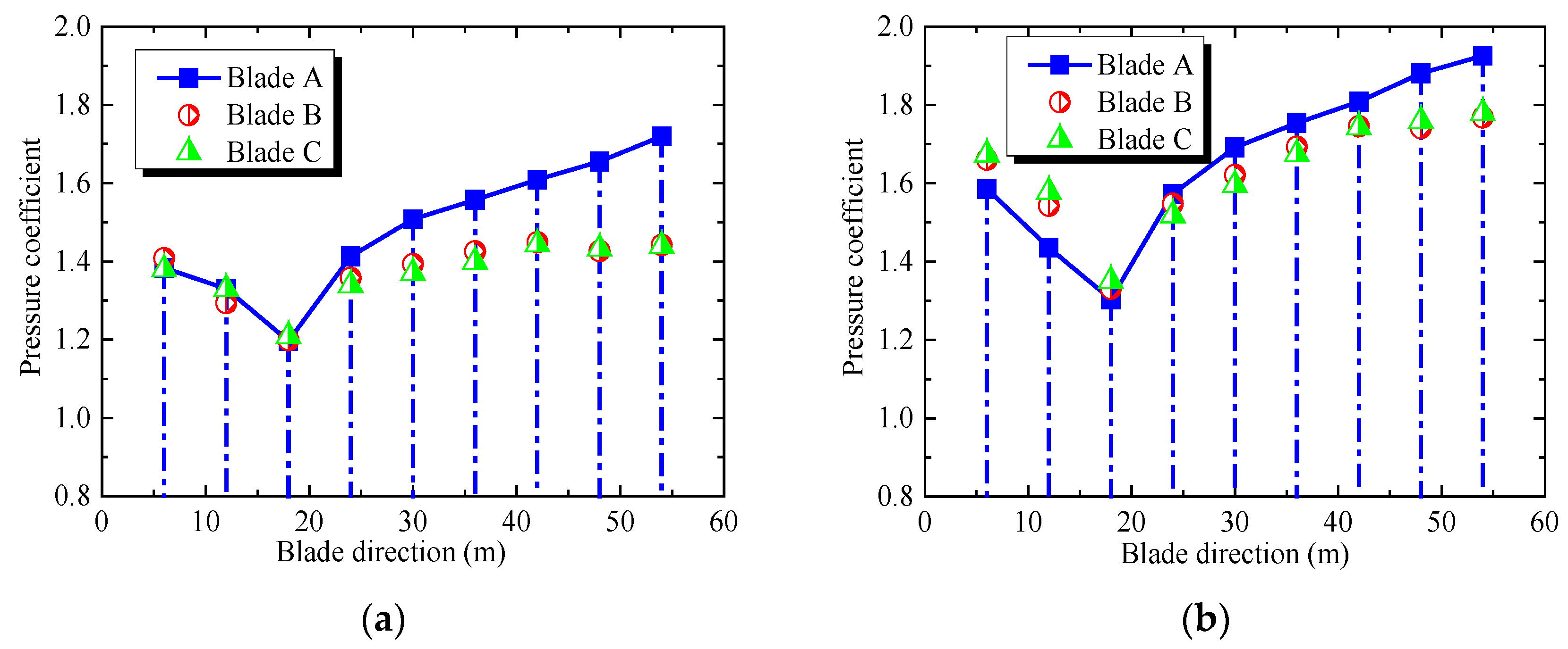
Figure 16.
Distribution curves of overall wind pressure coefficient on blades under normal wind and typhoon loads. (a) Normal wind; (b) Typhoon.
Figure 16.
Distribution curves of overall wind pressure coefficient on blades under normal wind and typhoon loads. (a) Normal wind; (b) Typhoon.
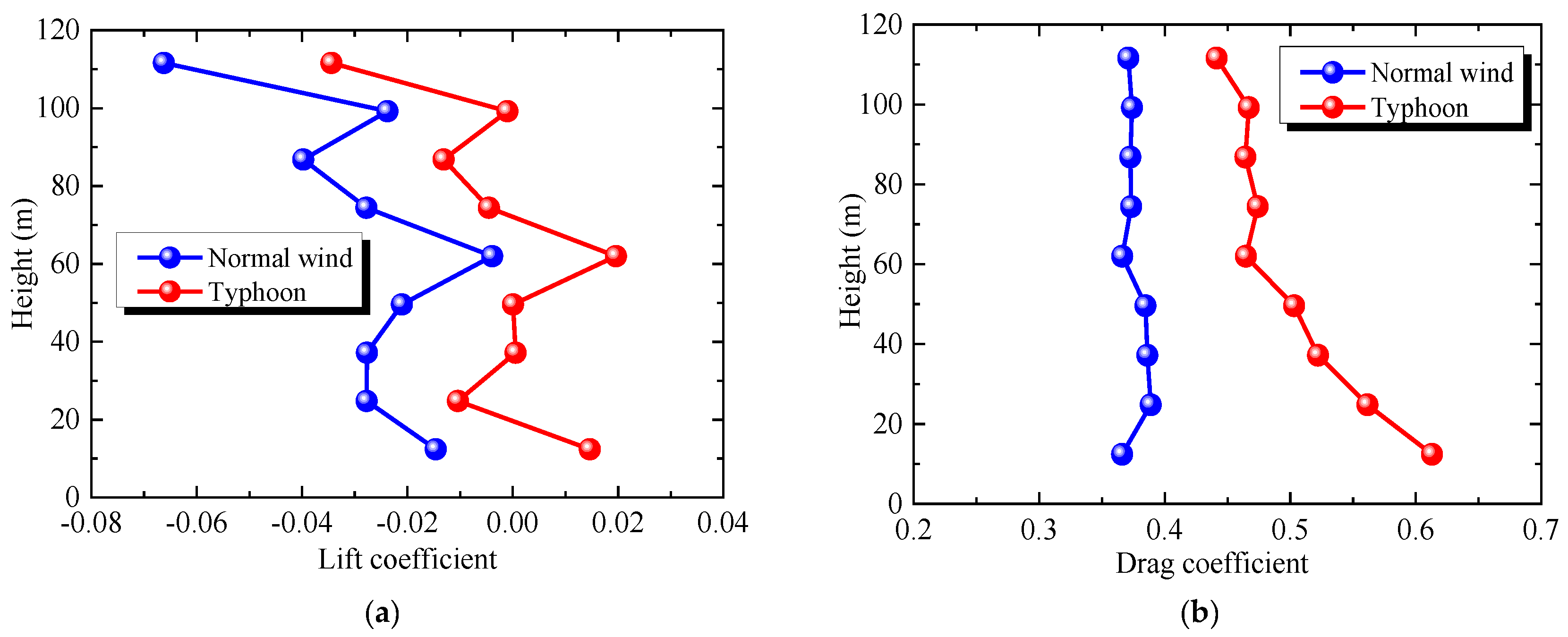
Figure 17.
Distribution curves of lift coefficient and drag coefficient of the tower body under normal wind and typhoon loads. (a) Lift coefficient. (b) Drag coefficient.
Figure 17.
Distribution curves of lift coefficient and drag coefficient of the tower body under normal wind and typhoon loads. (a) Lift coefficient. (b) Drag coefficient.
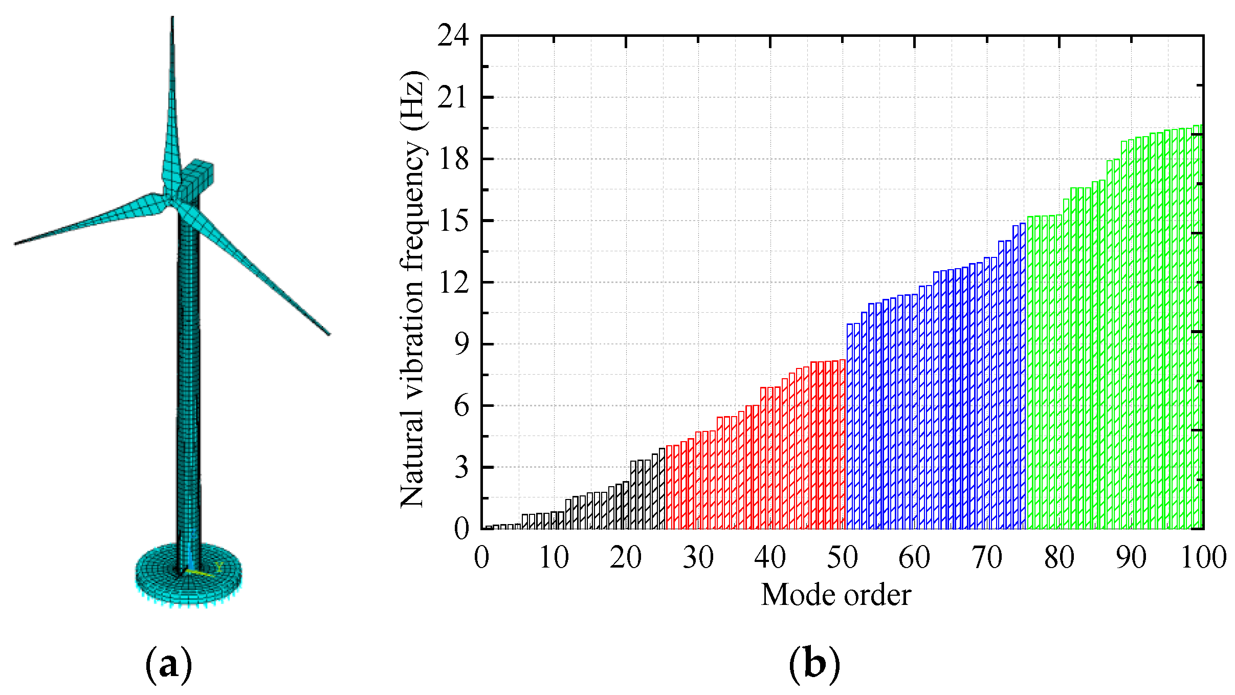
Figure 18.
Finite element model of wind turbine and the first 100 orders of inherent frequency. (a) Finite element model; (b) First 100 orders of inherent frequency.
Figure 18.
Finite element model of wind turbine and the first 100 orders of inherent frequency. (a) Finite element model; (b) First 100 orders of inherent frequency.
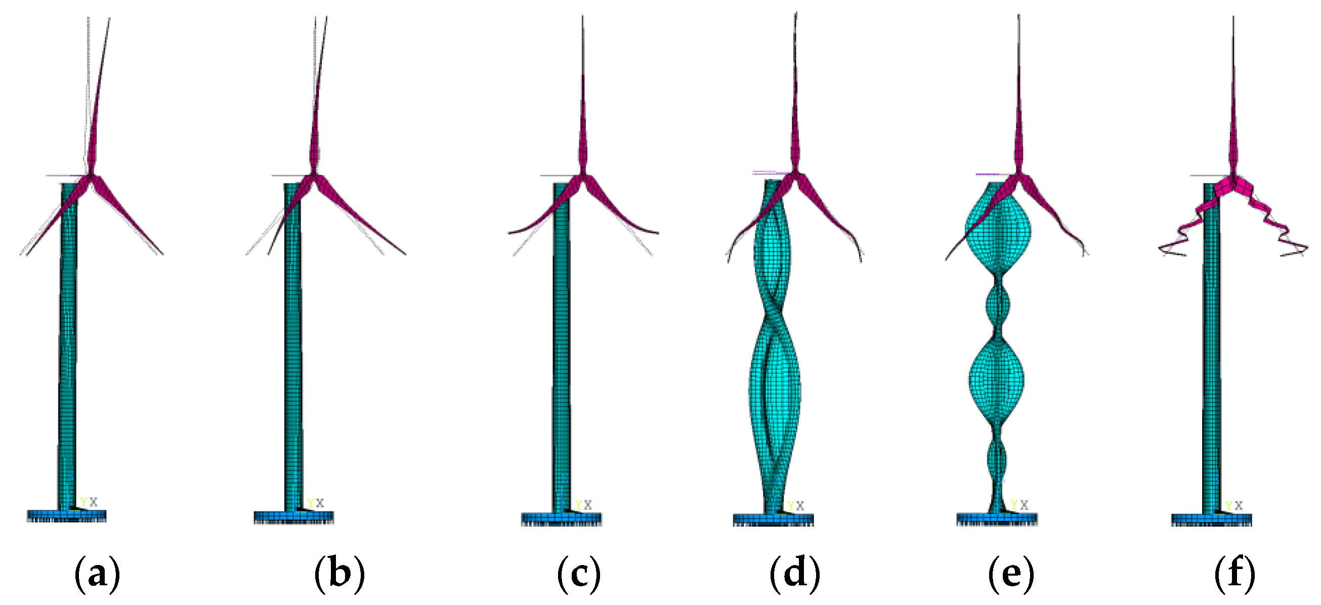
Figure 19.
Mode of vibration of the tower–blade coupling model at different orders. (a) First order; (b) Fifth order; (c) 10th order; (d) 30th order; (e) 50th order; (f) 100th order.
Figure 19.
Mode of vibration of the tower–blade coupling model at different orders. (a) First order; (b) Fifth order; (c) 10th order; (d) 30th order; (e) 50th order; (f) 100th order.
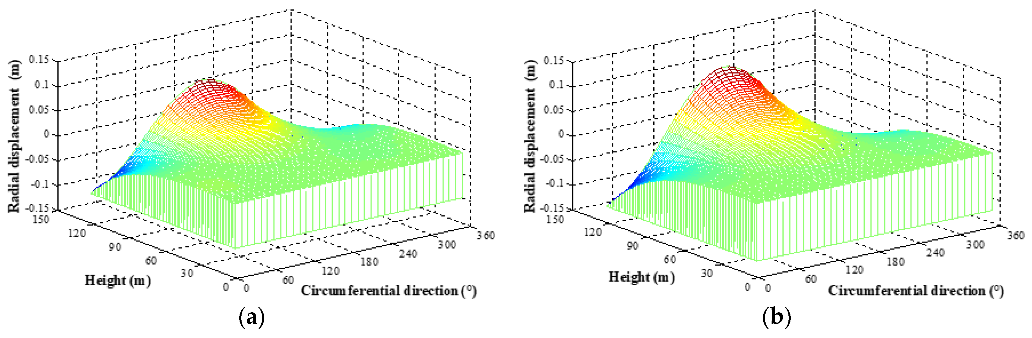
Figure 20.
3D radial displacement of tower body under normal wind and typhoon loads. (a) Normal wind; (b) Typhoon.
Figure 20.
3D radial displacement of tower body under normal wind and typhoon loads. (a) Normal wind; (b) Typhoon.
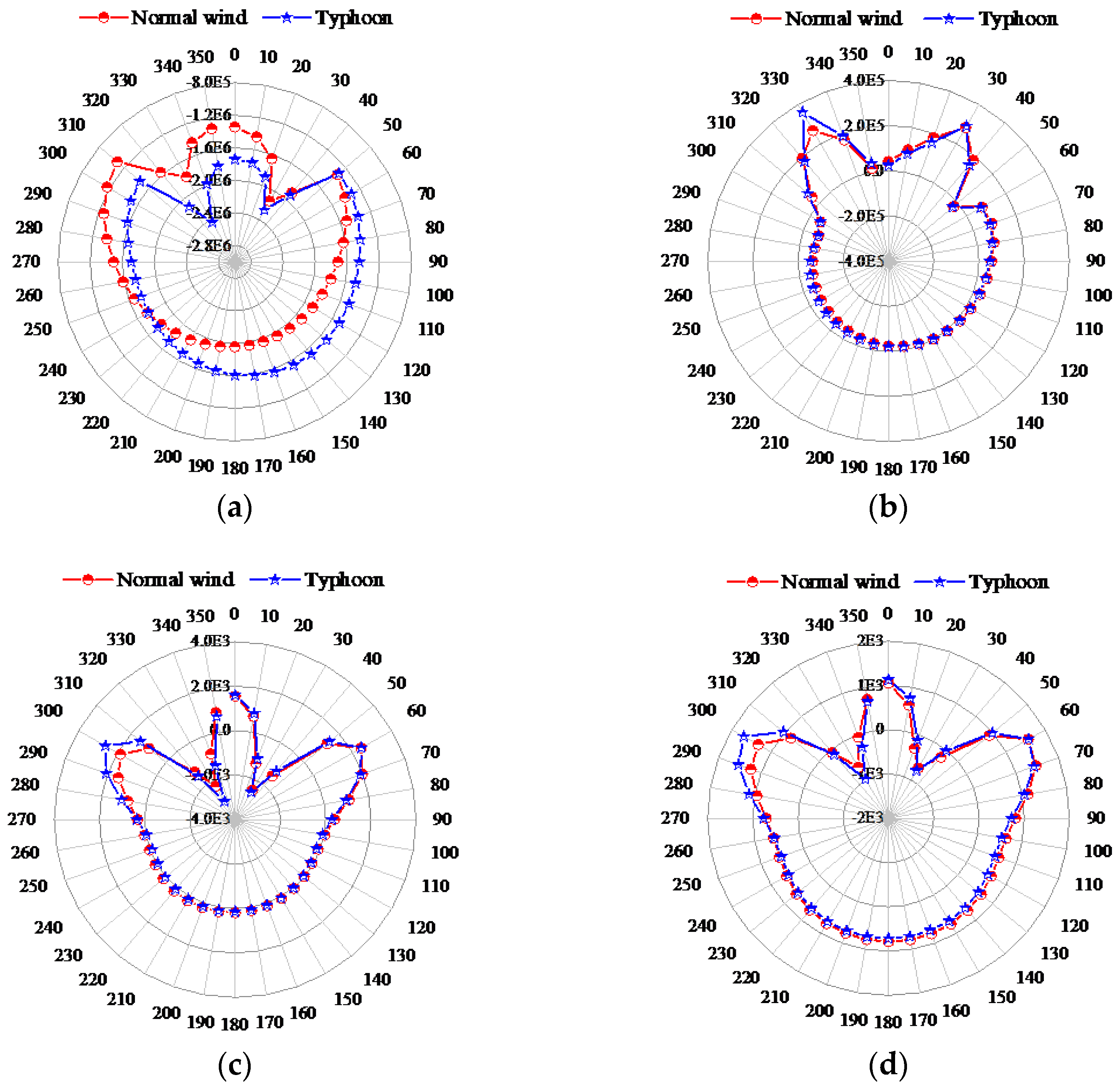
Figure 21.
Internal stress responses at the tower bottom of the wind turbine system under normal wind and typhoon loads. (a) Meridian axial force Ty/(N); (b) Shearing force Txy/(N); (c) Circumferential bending moment Mx/(N·m); (d) Meridian bending moment My/(N·m).
Figure 21.
Internal stress responses at the tower bottom of the wind turbine system under normal wind and typhoon loads. (a) Meridian axial force Ty/(N); (b) Shearing force Txy/(N); (c) Circumferential bending moment Mx/(N·m); (d) Meridian bending moment My/(N·m).
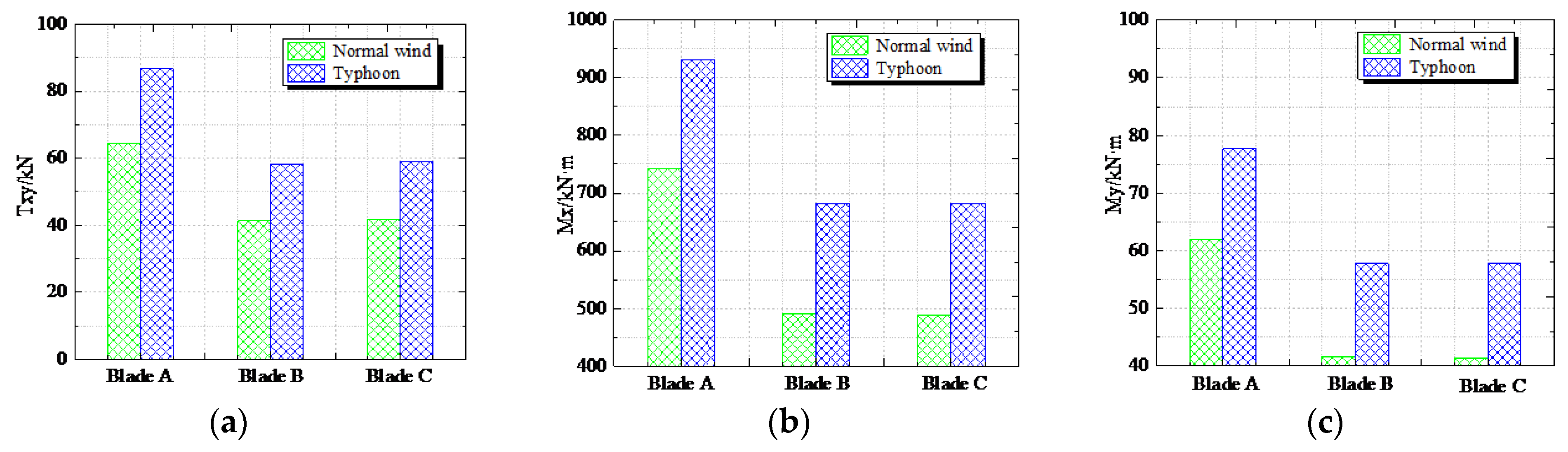
Figure 22.
Internal stress responses at the blade roots of the wind turbine under normal wind and typhoon loads. (a) Shearing force (Txy); (b) Circumferential bending moment (Mx); (c) Meridian bending moment (My).
Figure 22.
Internal stress responses at the blade roots of the wind turbine under normal wind and typhoon loads. (a) Shearing force (Txy); (b) Circumferential bending moment (Mx); (c) Meridian bending moment (My).
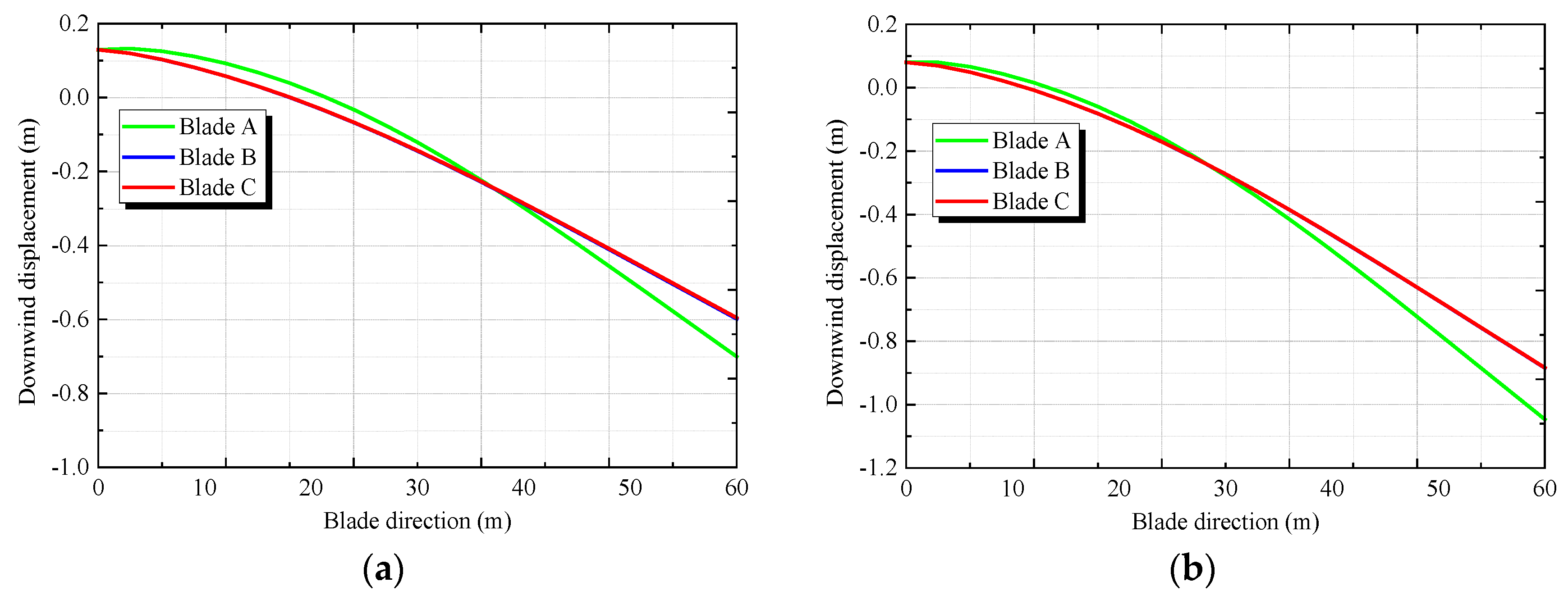
Figure 23.
Distribution curves of downwind displacements of three blades under normal wind and typhoon loads. (a) Normal wind; (b) Typhoon.
Figure 23.
Distribution curves of downwind displacements of three blades under normal wind and typhoon loads. (a) Normal wind; (b) Typhoon.
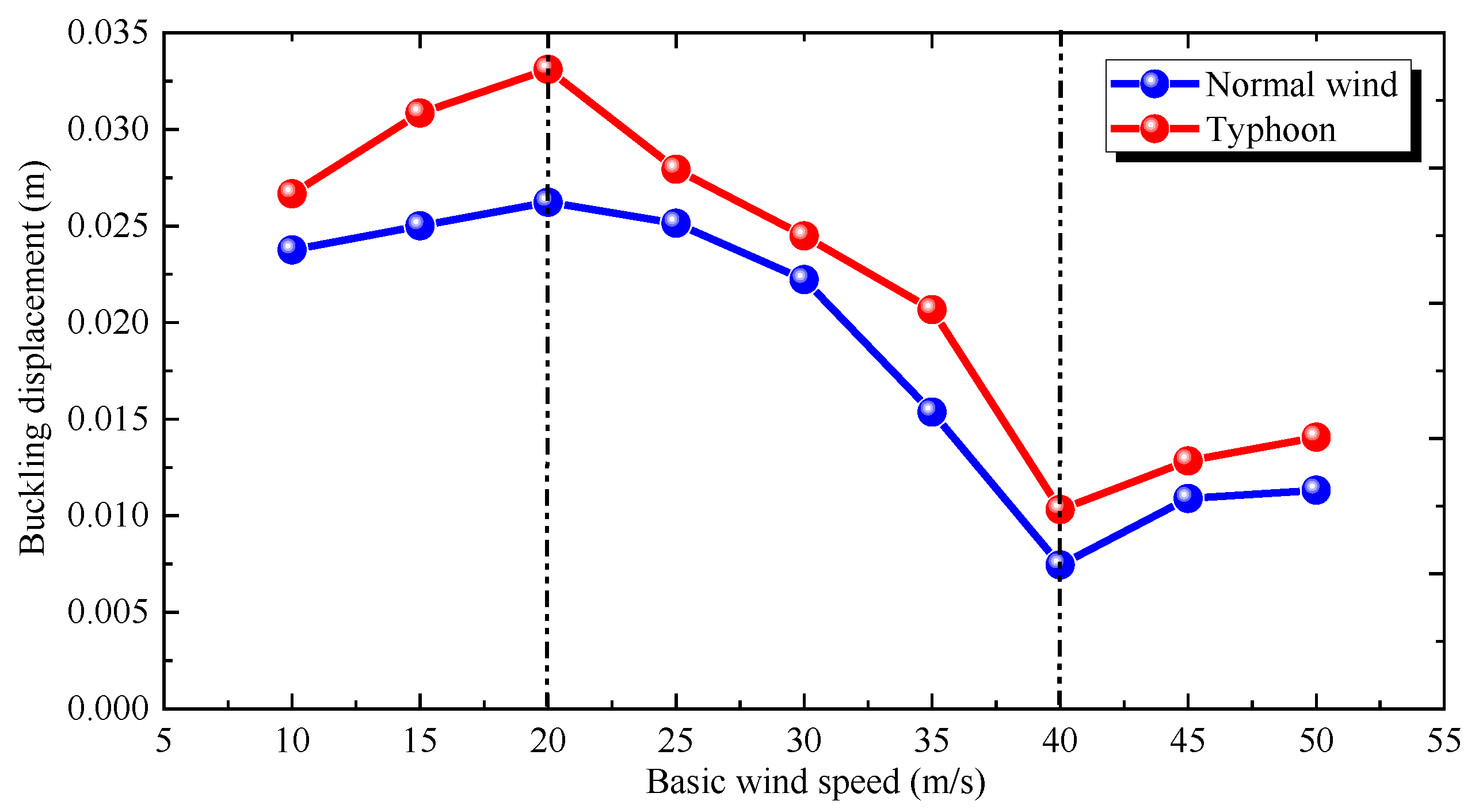
Figure 24.
Changes of the buckling displacement of the wind turbine with wind speed under normal wind and typhoon loads.
Figure 24.
Changes of the buckling displacement of the wind turbine with wind speed under normal wind and typhoon loads.
Table 1.
Altitudes of different vertical layers.
Table 1.
Altitudes of different vertical layers.
| Layers | Altitude/m | Layers | Altitude/m |
|---|
| 0 | 0 | 19 | 997.85 |
| 1 | 5.41 | 20 | 1441.03 |
| 2 | 21.64 | 21 | 1864.44 |
| 3 | 43.28 | 22 | 2383.35 |
| 4 | 64.96 | 23 | 2929.90 |
| 5 | 86.67 | 24 | 3508.54 |
| 6 | 108.42 | 25 | 4124.07 |
| 7 | 130.20 | 26 | 4780.99 |
| 8 | 152.01 | 27 | 5484.65 |
| 9 | 179.34 | 28 | 6243.02 |
| 10 | 217.70 | 29 | 7067.05 |
| 11 | 272.71 | 30 | 8489.99 |
| 12 | 350.13 | 31 | 10,070.22 |
| 13 | 439.15 | 32 | 11,332.60 |
| 14 | 528.81 | 33 | 12,805.37 |
| 15 | 619.11 | 34 | 14,592.36 |
| 16 | 710.08 | 35 | 17,014.78 |
| 17 | 824.83 | 36 | 19,617.33 |
| 18 | 987.29 | 37 | —— |
Table 2.
Physical parameter settings of the WRF model.
Table 2.
Physical parameter settings of the WRF model.
| WRF Parameters | Main Zone (D01) | Nesting Zone (D02) | Nesting Zone (D03) |
|---|
| Horizontal resolution | 13.5 km | 4.5 km | 1.5 km |
| Integral time step | 180 s |
| Microphysical process scheme | Lin |
| Long-wave radiation | RRTM |
| Short-wave radiation | Dudhia |
| Near-ground layer scheme | Monin-Obukhov |
| Land surface process scheme | Noah |
| Planet boundary layer scheme | MYJ |
| Cumulus convective parameterization scheme | Kain-Fritsch |
Table 3.
Main structural design parameters and model of the five-MW wind turbine.
Table 3.
Main structural design parameters and model of the five-MW wind turbine.
| Parameters | Numerical Value | 3D Blade Model | 3D Wind Turbine Model |
|---|
| Tower height | 124 m | ![Applsci 08 01982 i001]() | ![Applsci 08 01982 i002]() |
| Radius at tower top | 3.0 m |
| Radius at tower bottom | 3.5 m |
| Thickness at tower top | 0.04 m |
| Thickness at tower bottom | 0.09 m |
| Blade length | 60 m |
| Nacelle size | 18 m × 6 m × 6 m |
| Cut-out speed | 25 m/s |
| Yaw rotation speed | 0.5°/s |
Table 4.
Blade parameters of wind turbine.
Table 4.
Blade parameters of wind turbine.
| Position/% | Blade Span/m | Chord Length/m | Installation Angle/° | Blade Pitch Angle/° | Position/% | Blade Span/m | Chord Length/m | Installation Angle/° | Blade Pitch Angle/° |
|---|
| 5 | 3 | 2.9 | 0.823 | 37.14 | 55 | 33 | 1.95 | 0.169 | −0.293 |
| 10 | 6 | 3.66 | 0.64 | 26.672 | 60 | 36 | 1.75 | 0.156 | −1.072 |
| 15 | 9 | 4.41 | 0.507 | 19.069 | 65 | 39 | 1.58 | 0.144 | −1.736 |
| 20 | 12 | 4.56 | 0.414 | 13.692 | 70 | 42 | 1.42 | 0.134 | −2.31 |
| 25 | 15 | 4.25 | 0.346 | 9.83 | 75 | 45 | 1.27 | 0.125 | −2.81 |
| 30 | 18 | 3.91 | 0.296 | 6.976 | 80 | 48 | 1.12 | 0.118 | −3.25 |
| 35 | 21 | 3.59 | 0.258 | 4.802 | 85 | 51 | 0.98 | 0.111 | −3.64 |
| 40 | 24 | 3.05 | 0.229 | 3.103 | 90 | 54 | 0.83 | 0.105 | −3.987 |
| 45 | 27 | 2.63 | 0.205 | 1.742 | 95 | 57 | 0.69 | 0.099 | −4.299 |
| 50 | 30 | 2.29 | 0.186 | 0.63 | 100 | 60 | 0.54 | 0.095 | −4.58 |
Table 5.
Grid number, grid quality, and windward pressure coefficient on the tower body under different meshing schemes.
Table 5.
Grid number, grid quality, and windward pressure coefficient on the tower body under different meshing schemes.
| Meshing Schemes | 1 | 2 | 3 | 4 | 5 |
|---|
| Total number of grids | 1.1 million | 4.5 million | 7.4 million | 9.3 million | 28.4 million |
| Minimum orthogonal quality of grids | 0.13 | 0.36 | 0.53 | 0.60 | 0.64 |
| Grid skewness | 0.95 | 0.87 | 0.82 | 0.74 | 0.71 |
| Windward pressure coefficient | 0.92 | 0.88 | 0.85 | 0.80 | 0.79 |
Table 6.
Lift–drag coefficient ratio of the tower body under normal wind and typhoon loads.
Table 6.
Lift–drag coefficient ratio of the tower body under normal wind and typhoon loads.
| CL/CD | Height of the Tower Body |
|---|
| 12.4 m | 24.8 m | 37.2 m | 49.6 m | 62 m | 74.4 m | 86.8 m | 99.2 m | 111.6 m |
|---|
| Normal wind | −0.040 | −0.071 | −0.072 | −0.055 | −0.011 | −0.074 | −0.107 | −0.064 | −0.179 |
| Typhoon loads | 0.024 | −0.019 | 0.001 | 0.001 | 0.042 | −0.010 | −0.028 | −0.002 | −0.078 |
Table 7.
Downwind displacements at blade tips under normal wind and typhoon loads.
Table 7.
Downwind displacements at blade tips under normal wind and typhoon loads.
| Blade A | Blade B | Blade C |
|---|
| Normal Wind | Typhoon | Normal Wind | Typhoon | Normal Wind | Typhoon |
|---|
| −0.701 m | −1.047 m | −0.599 m | −0.885 m | −0.596 m | −0.884 m |
Table 8.
Comparison of buckling mode and eigenvalues of wind turbine system under normal wind and typhoon loads.
Table 8.
Comparison of buckling mode and eigenvalues of wind turbine system under normal wind and typhoon loads.
| Buckling Eigenvalue under Normal Wind | Buckling Mode under Normal Wind | Buckling Mode under Typhoon Loads | Buckling Eigenvalue under Typhoon Loads |
|---|
| Buckling coefficient | 2.955 | ![Applsci 08 01982 i003]() | ![Applsci 08 01982 i004]() | Buckling coefficient | 2.992 |
| Critical wind speed/(m/s) | 24.12 | Critical wind speed/(m/s) | 31.57 |
| Maximum displacement/m | 0.025 | Maximum displacement/m | 0.032 |


