Classification of Heart Sound Signal Using Multiple Features


Department of Digital Contents, Sejong University, Seoul 05006, Korea
*
Author to whom correspondence should be addressed.
Appl. Sci. 2018, 8(12), 2344; https://0-doi-org.brum.beds.ac.uk/10.3390/app8122344
Submission received: 10 October 2018
/
Revised: 17 November 2018
/
Accepted: 20 November 2018
/
Published: 22 November 2018
(This article belongs to the Special Issue Deep Learning and Big Data in Healthcare)
Abstract
:Cardiac disorders are critical and must be diagnosed in the early stage using routine auscultation examination with high precision. Cardiac auscultation is a technique to analyze and listen to heart sound using electronic stethoscope, an electronic stethoscope is a device which provides the digital recording of the heart sound called phonocardiogram (PCG). This PCG signal carries useful information about the functionality and status of the heart and hence several signal processing and machine learning technique can be applied to study and diagnose heart disorders. Based on PCG signal, the heart sound signal can be classified to two main categories i.e., normal and abnormal categories. We have created database of 5 categories of heart sound signal (PCG signals) from various sources which contains one normal and 4 are abnormal categories. This study proposes an improved, automatic classification algorithm for cardiac disorder by heart sound signal. We extract features from phonocardiogram signal and then process those features using machine learning techniques for classification. In features extraction, we have used Mel Frequency Cepstral Coefficient (MFCCs) and Discrete Wavelets Transform (DWT) features from the heart sound signal, and for learning and classification we have used support vector machine (SVM), deep neural network (DNN) and centroid displacement based k nearest neighbor. To improve the results and classification accuracy, we have combined MFCCs and DWT features for training and classification using SVM and DWT. From our experiments it has been clear that results can be greatly improved when Mel Frequency Cepstral Coefficient and Discrete Wavelets Transform features are fused together and used for classification via support vector machine, deep neural network and k-neareast neighbor(KNN). The methodology discussed in this paper can be used to diagnose heart disorders in patients up to 97% accuracy. The code and dataset can be accessed at “https://github.com/yaseen21khan/Classification-of-Heart-Sound-Signal-Using-Multiple-Features-/blob/master/README.md”.
1. Introduction
Cardiovascular system is a perpetual source of data that sanctions soothsaying or distinguishing among cardiovascular diseases. External constrains can lead to cardiac diseases that can cause sudden heart failure [1]. Cardiovascular diseases are censorious and must be detected with no time delay [2]. Heart diseases may be identified by elucidating the cardiac sound data. The heart sound signal characteristics may vary with respect to different kinds of heart diseases. A huge difference in the pattern can be found between a normal heart sound signal and abnormal heart sound signal as their PCG signal varies from each other with respect to time, amplitude, intensity, homogeneity, spectral content, etc [3].
Cardiovascular auscultation is the principal yet simple diagnosing method used to assess and analyze the operation and functionality of the heart. It is a technique of listening to heart sound with stethoscope. The main source of the generation of heart sound is due to unsteady moment of blood called blood turbulence. The opening and closing of atrioventricular values, mitral and tricuspid values causes differential blood pressure and high acceleration and retardation of blood flow [4]. The auscultation of cardiac disorders is carried out using an electronic stethoscope which is indeed cost effective and non-invasive approach [3]. The digital recording of heart sound with the help of electronic stethoscope is called PCG [4].
Once the heart sound is obtained, it can be classified via computer aided software techniques, these techniques need more accurately defined heart sound cycle for feature extraction process [3]. Many different automated classifying approaches have been used, including artificial neural network (ANN) and hidden Markov model (HMM). Multilayer perceptron-back propagation (MLP-BP), Wavelet coefficients and neural networks were used for classification of heart sound signal. But they have often resulted in lower accuracy due to segmentation error [2].
To achieve better accuracy, in this work, we propose SVM, centroid displacement based KNN and DNN based classification algorithm using discrete wavelets transform (DWT) and (MFCC) features. The recognition accuracy can be increased for both noisy and clear speech signals, using discrete wavelets transform fused together with MFCCs features [5,6]. We extracted MFCCs features and discrete wavelets transform features for heart sound signals (normal and abnormal) and classified them using support vector machine, deep neural network and centroid displacement based KNN, the highest accuracy we achieved so far is 97.9%.
The beginning of this paper describes some background knowledge about heart sound signal processing and categories of heart disorders in brief detail, afterwards the methodology of features (MFCCs and DWT) and classifiers we used is discussed. In the experiment section we talk about classification of features, detail about classifiers, the tools we used, and database in detail. In the end, we have discussed our results and performance evaluation using accuracy and averaged F1 score and the last paragraph concludes the paper.
2. Background
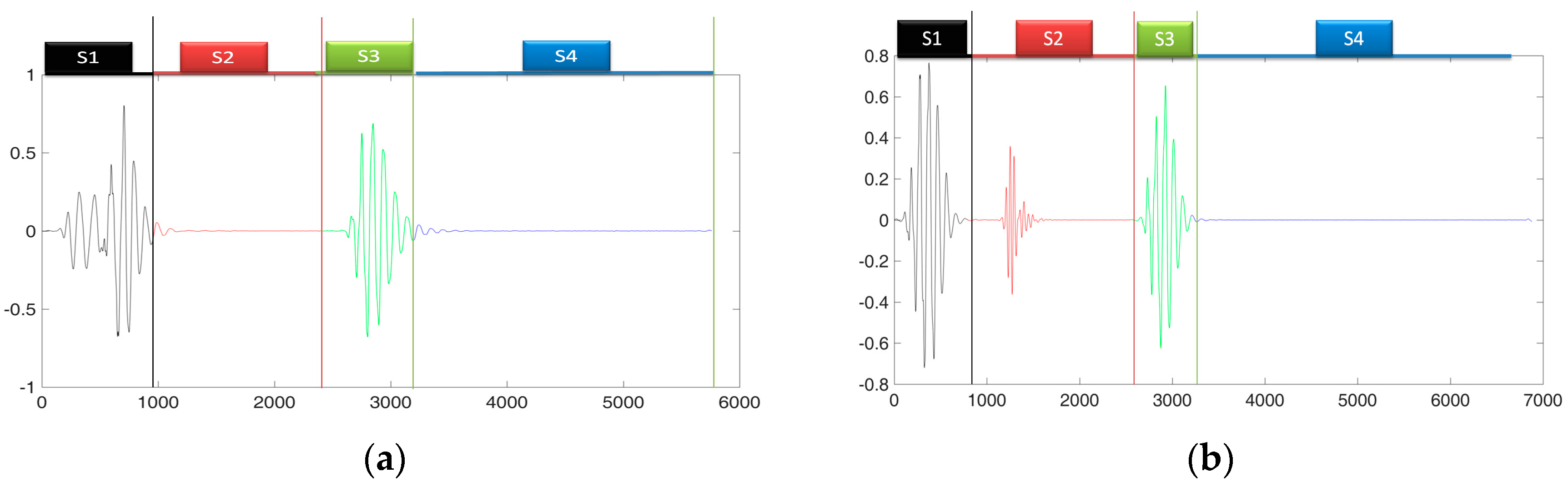
The human heart is comprised of four chambers. Two of them are called atrias and they make the upper portion of the heart while remaining two chambers are called ventricles and they make lower portion of heart, and blood enters the heart through atrias and exit through ventricles. Normal heart sounds (Figure 1a is an example of normal heart sound signal) are generated by closing and opening of the valves of heart. The heart sound signals produced, are directly related to opening and closing of the valves, blood flow and viscosity. Therefore during exercise or other activities which increases the heart rate, blood flow through the valves is increased and hence heart sound signal’s intensity is increased and during shock (low blood flow) the sound signal’s intensity is decreased [2]. Figure 1f also shows the spectrum of a PCG signal.
The movements of heart valves generate audible sounds of frequency range lower than 2 kHz, commonly refer to as “lub-dub” The “lub” is the first portion in the heart sound signal and is denoted by (S1), it is generated from the closing of mitral and tricuspid valve. One complete cardiac cycle is the heart sound signal wave which starts from S1 and ends to the start of next S1 and it is described as one heartbeat. The duration, pitch, and shape of the heart sound shows us detail about the different conditions of heart [4]. Closing of mitral valves is followed by closing of tricuspid valve and usually the delay between this operation is 20 to 30 ms. Due to the left ventricle contraction first, the mitral valve component occurs first followed by tricuspid valve component in the signal. If the duration between these two sound components is in between 100 to 200 ms, it is called a split and its frequency range lies from 40 to 200 Hz and it is considered fatal if the delay is above 30 ms [7]. “Dub”, is generated (the second heart sound component denoted by “S2”), when the aortic vales and pulmonary valves are closed. S1 is usually of longer time period and lower frequency than S2 which has shorter duration but higher frequency ranges (50 to 250 Hz). A2 is another heart sound signal component generated due to movement of Aortic valve and P2 is another heart sound signal component generated due to movement of pulmonary valve. Aortic pressure is higher compared to pulmonary pressure hence the A2 component appears before P2 in the heart sound signal. The presence of cardiac diseases such as pulmonary stenosis and atrial septal defect can be identified by analyzing closely the split between aortic component A2 and pulmonary component P2 and their intensities. During deep emotional and excitement state, the duration between A2 and P2 may be longer than usual, causing long and wide splitting in between the components. This state is considered fatal if the delay between these component is longer than 30 ms [7].
Beside “lub-dub”, some noisy signals may be present in the heart sounds called murmurs. Murmurs, both normal and fatal, are continuous vibrations produced due to the irregular flow of blood in cardiovascular system. Murmurs can be of two types “normal murmurs” and “abnormal murmurs”, normal murmurs are usually present in heart sound signal component of infants, children and adults during exercise also in women (during pregnancy), this type of murmur can be detected in the first heart sound. Abnormal murmurs are usually present in heart patience which indicate a heart valve defect called stenosis (squeezed heart valves) and regurgitation (bleeding heart valves) [7]. Murmurs are the unusual sound present in heart sound cycle of an abnormal heart sound which indicates some abnormalities. Based on the murmur position in the heart cycle, they can be called systolic murmurs, diastolic murmurs and continuous murmurs [4]. These murmurs sounds and clicks are a key points to identify cardiovascular disease [7]. Murmurs in the heart sound can be discovered using stethoscope, echocardiography or phonocardiography.
Murmurs are classified as continuous murmurs, systolic murmurs and diastolic murmurs. Systolic murmurs are present during systole and they are generated during the ventricles contraction (ventricular ejection). In the heart sound component they are present between S1 and S2 hence are called as systolic murmurs. Based on their types, these systolic murmurs can be called as either ejection murmurs (atrial septal defect, pulmonary stenosis, or aortic stenosis) Figure 1e, or regurgitant murmurs (ventricular septal defect, tricuspid regurgitation, mitral regurgitation or mitral valve prolapse) Figure 1c.
Diastolic murmurs are created during diastole (after systole), when the ventricles relax. Diastolic murmurs are present between the second and first heart sound portion, this type of murmur is usually due to mitral stenosis (MS) or aortic regurgitation (AR) by as shown in Figure 1d. Mitral valve prolapse (MVP) is a disease where the murmur sound is present in between the systole section as shown in Figure 1b. The murmur of AR is high pitched and the murmur of AS is low pitched. In mitral regurgitation (MR), systolic component S1 is either soft or buried or absent, and the diastolic component S2 is widely split. In mitral stenosis, the murmur is low pitched and rumbling and is present along the diastolic component. In mitral valve prolapse, the murmur can be found throughout S1compnent. The sound signal of VSD and MR are mostly alike [2,7].
Summarizing the above discussion, we can see that heart sound signal can be acquired using and electronic stethoscope, in each complete cycle of heart sound signal we have S1–S4 intervals, S3 and S4 are rare heart sounds and are not normally audible but can be shown on the graphical recording i.e., phonocardiogram [4]. S3 and S4 intervals are called murmur sound and the heart sound signal which carries murmurs are called abnormal heart sounds and can be classified according to murmur position in the signal. In this study automatic classification of heart sound signal is carried out using five categories, one normal category and four abnormal categories. These abnormal categories are aortic stenosis (AS), mitral regurgitation (MR), mitral stenosis (MS) and MVP (murmur exist in the systole interval). Figure 1 shows graphical representation of theses heart sound signals categorically.
The classification of heart sound signal can be carried out by several machine learning classifiers available for biomedical signal processing. One of them is SVM which can be used for classification of heart sounds. SVM is machine learning, classification and recognition technique that totally works on statistical learning and theorems, the classification accuracy of SVM is much more efficient than conventional classification techniques [8]. Another classifier that recently gained attention is DNN, DNN acoustic models have high performance in speech processing as well as other bio medical signal processing [9]. In this paper, our study shows that these classifiers (SVM and DNN also centroid displacement based KNN) have good performance for heart sound signal classification. The performance of Convolutional Neural Network is optimized for image classification, so this method is not suitable for the feature set we used in this paper. We also used Recurrent Neural Network in the pilot test, but our DNN method showed better results [10,11].
3. Methodology
The heart sound signal contains useful data about the working and health status of the heart, the heart sound signal can be processed using signal processing approach to diagnose various heart diseases before the condition of the heart get worse. Hence, various signal processing techniques can be applied to process the PCG signal. The stages involved in processing and diagnosing the heart sound signal are, the acquisition of heart sound signal, noise removal, sampling the PCG signal at a specific frequency rate, feature extraction, training and classification. As shown in the following Figure 2.
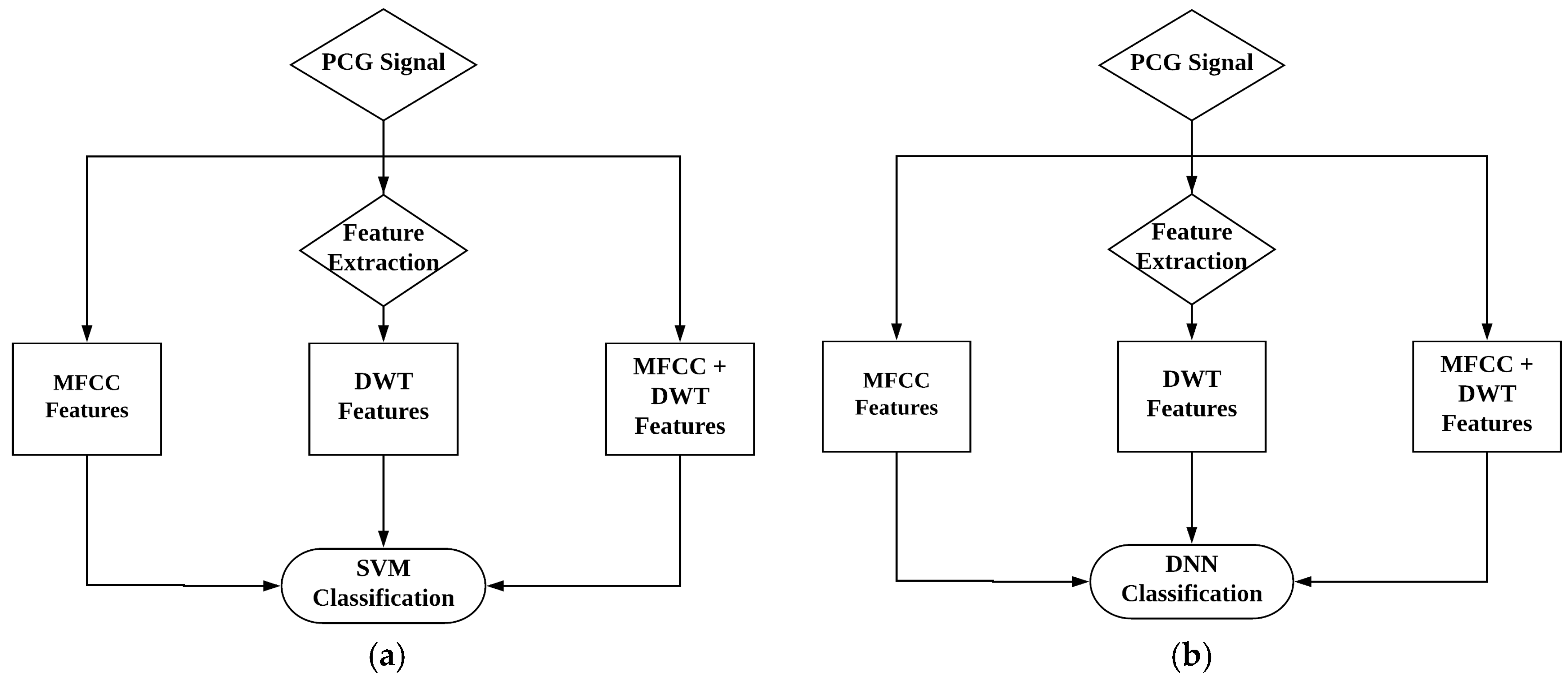
From heart sound signal we extract two different types of features: MFCCs and DWT. To classify these features we used SVM, centroid displacement based KNN and DNN as classifiers. For performance evaluation of features using these classifiers, we carried out our experiment and evaluated the averaged F1 score and accuracy for all of the three features (MFCCs, DWT and a combination of these) using the three classifies (SVM, DNN and centroid based KNN).
3.1. Mel Frequency Cepstral Coefficients (MFCCs)
We extracted features as a set of measured, non-redundant and derived values from heart signal which has been used in our study. As we used two types of features, MFCCs, DWT and the combination of both, MFCCs features are enormously used in signal processing and recognition. They were first calculated and used in speech analysis by Davis and Mermelstein in the 1980’s. Human can recognize small changes in pitch of sound signal at lower frequencies and the MFCC scale is linear for those frequencies having range <1 kHz. The power aspect of MFCCs is that they are able to represent the signal information efficiently. The MFCCs feature are almost similar to the log filter bank energies and include the mel scale which makes it an exact copy on smaller scale of what humans understand, the frequency in mel scale is given by Equation (1):
In MFCC algorithm, using Hamming window an audio signal is reshaped to smaller windows hence splitting of signal to frames is done. Using Fast Fourier Transform, spectrum is computed for each frame, using filter bank each spectrum is being weighted. Finally using Logarithm and Discrete Cosine Transform, the MFCC vector is computed [12,13]. Compared to other features, MFCCs have good performance against noisy signal when used in speech signal processing hence can be used in biomedical signal processing [12]. During feature extraction, we resampled each signal frequency to 8 KHz, the length of the each signal’s feature extracted is 19 and the length of frame in each sample is 240 and the step size is 80. The following diagram represents the extraction of MFCCs features Figure 3a.
3.2. Discrete Wavelets Transform (DWT)
DWT is mathematical tool for decomposing data in a top down fashion. DWT represent a function in terms of a rough overall form, and a wide range of details. Despite of the requirement and type of function i.e., signals images etc. DWT offers sublime methodology and technique for representing the amount of detail present [14]. Wavelets perform and offer scale based analysis for a given data. A wide range of applications and usage has been found for these wavelets including signal processing, mathematics and numerical analysis and, for its better performance in signals and image processing it is considered an alternative to Fast Fourier Transform as DWT provide time-frequency representation [15]. When there is a need for processing and analyzing non stationary tool, DWT can be used [16]. Study shows that discrete wavelets transform have high performance in speech signal processing so far and especially when combined with MFCCs, the performance is boosted further [5].
DWT can be defined as a short wave which carries its energy and information condensed in time. They are limited in space and possessing an average value approaching to zero. Each signal contains two components i.e., low frequency and high frequency components. Low frequency components mostly contain maximum information part, and high frequency components convey quality. That is why in DWT estimation and details are being rated. The estimation is of the high-scale, low-frequency components of the signal and the Details are the low-scale, high-frequency components. In Figure 3b, it is shown that down sampling a given signal can be divided into its component at level one it has cA1, cD1 approximated and detailed components and at level two it has cA2 and cD2 estimated and detailed components. Down sampling ensures the absence of redundancy in a given data [17]. Mathematically, DWT can be expressed in the following Equation (2) as:
The above equation can be used to extract more useful data from audio signal using DWT [18]. In case of DWT the length of feature vector is 24.
3.3. Support Vector Machine (SVM)
Its working is based on Statistics Learning Theory (SLT) and structure risk minimization principal (SRMP), it is considered a unique method in machine learning for signal processing. It has unique performance in solving nonlinear learning problems and sample learning problems [19,20]. Based on optimization technology SVM is a unique tool in solving machine learning challenges. It has been first used by Vapnik in 1990’s and now days they are used in pattern recognition in image processing and signal processing. Based on SLT and SRMP, it can solve many complex structures, process big data appropriate to over learning [20]. The use of SVM has been started as hyper plane classifier and is useful in a situation where data is required to be separated linearly [21].
Suppose having sample Si and its sorts Ti, expressed as (Si, Ti), S Rd, Ti (1, −1), i = 1,…,N. The d is dimension number of input space. For standard SVM, its classifying border or edge is . Making the classifying borer or edge to maximum is equal to making the 2 to minimum. Therefore, the optimization problem of making the classifying edge to maximum can be expressed in the follow quadratic programming problem:
Subject to
where i 0 (i = 1, …, N ) is flexible variable, which ensures classification validity under linear non-separable case, and parameter C is a positive real constant which determines penalties to approximation errors, a higher value of C is similar as to assigning a higher penalty to errors. The function is a non-linear mapping function, by which the non-linear problem can be mapped as linear problem of a high dimension space. In the transforming space, we can get optimal hyper plane. The SVM algorithm can discern right classification to sample by solving above quadratic programming problem [21]. We choose nonlinear kernel (quadratic SVM) model for our experiments, in that case SVM needs another parameter gamma along with C to be optimized for better results. Both of these values greatly affect the classification decision of SVM, larger values of gamma brings classifier closer to training accuracy and lower values make it away from it [22]. Similarly lower values of C are more suitable in bringing decision function closer to training accuracy and vice versa. In our experiments we achieved good training accuracy using C values in range of 0.0003 to 0.0001 and gamma value of log103.
3.4. Deep Neural Network (DNN)
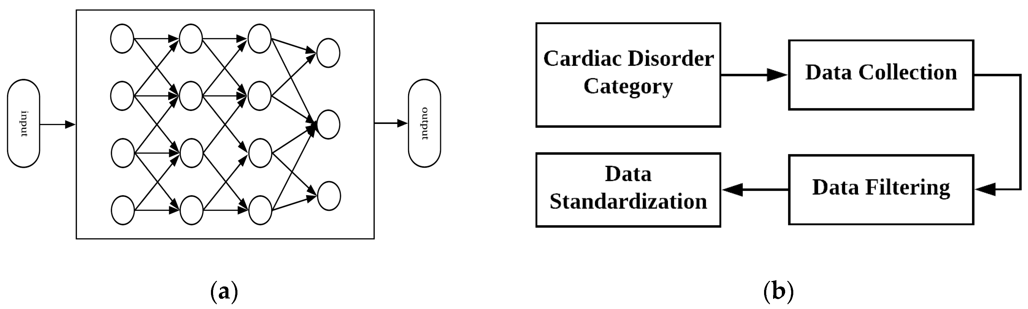
DNN is a new AI algorithm for machine learning and has been widely used in many research and developing fields. DNN is inspired bio natural object’s visual mechanism where it have many layers of neural network, it process data from their light carrying organs to center of the brain, replicating that mechanism, in DNN the process is done layer by layer where the information are carried out from one layer to another, sequentially extracting edge features, shape feature, part feature, and eventually forms abstract concept [23]. A DNN is a network of neurons in which they are grouped together in multiple layers, those layers are interconnected together in several sequential layers and neurons accepts the neuron activation from previous layer and calculate weighted sum multiply it with neuron and process the output to next layer and so on. The neurons in each layer of network combined execute a complex nonlinear mapping from the beginning to the last. This mapping causes the network to learn from neuron back propagation techniques using weighted sum of neurons. Figure 4a shows a simple neural network where there is an input to collection of many hidden layers and a final output.
For our DNN model we kept batch size equal to 100, three hidden layers and 2000 epochs for each training phase. We input the data to layers in chunks and the total numbers of chunks were calculated from the total number of features length divided by 40, as we selected the chunk size to be 40 for optimum results.
4. Experiments
We collected and arranged data in the form of database, which consist of two sets of data: normal set and abnormal set, the whole data in database (normal and abnormal) have five categories, one normal category (N) and four abnormal categories, the four abnormal categories were: aortic stenosis (AS) mitral stenosis (MS) mitral regurgitation (MR) mitral valve prolapse (MVP), details of data is shown in Table 1, there complete detail (w.r.t to category) were discussed in background section. The total numbers of audio files were 1000 for normal and abnormal categories (200 audio files/per category), the files are in .wav format. Our data collection procedure outline is shown in Figure 4b, in which we first selected cardiac disorder category, collected data then applied data standardization after filtering [Appendix A].
After gathering the data, the experiments we performed, can be categorized into nine types, as discussed in methodology section, we did first 3 experiments using SVM classifier and three types of features: MFCCs, DWT and MFCCs + DWT (fused features), second three experiments using DNN and last 3 experiments using centroid displacement based KNN, each of these features were trained and classified using each classifier individually. In case of centroid displacement based KNN we choose the value of k = 2.5 and that worked well for our dataset training. [24].
For training and classification of MFCCs features using SVM the parameters and arguments we used while extracting MFCCs features were as follows: sampling frequency 8000 Hz, feature vector having length 19 and frame size in sample 240 with step size of 80.Similarly, for training and classification of DWT features using SVM the parameters and arguments we used while extracting DWT features were as follows: sampling frequency 8000 Hz, and length of feature vector 24. Using fivefold cross validation technique, we classified our data using SVM and DNN. From dataset, 20% of sample data in each class was used for testing and eighty percent of sample data in each class for training, the performance of each machine learning algorithm with different features were recorded with respect to their given accuracies.
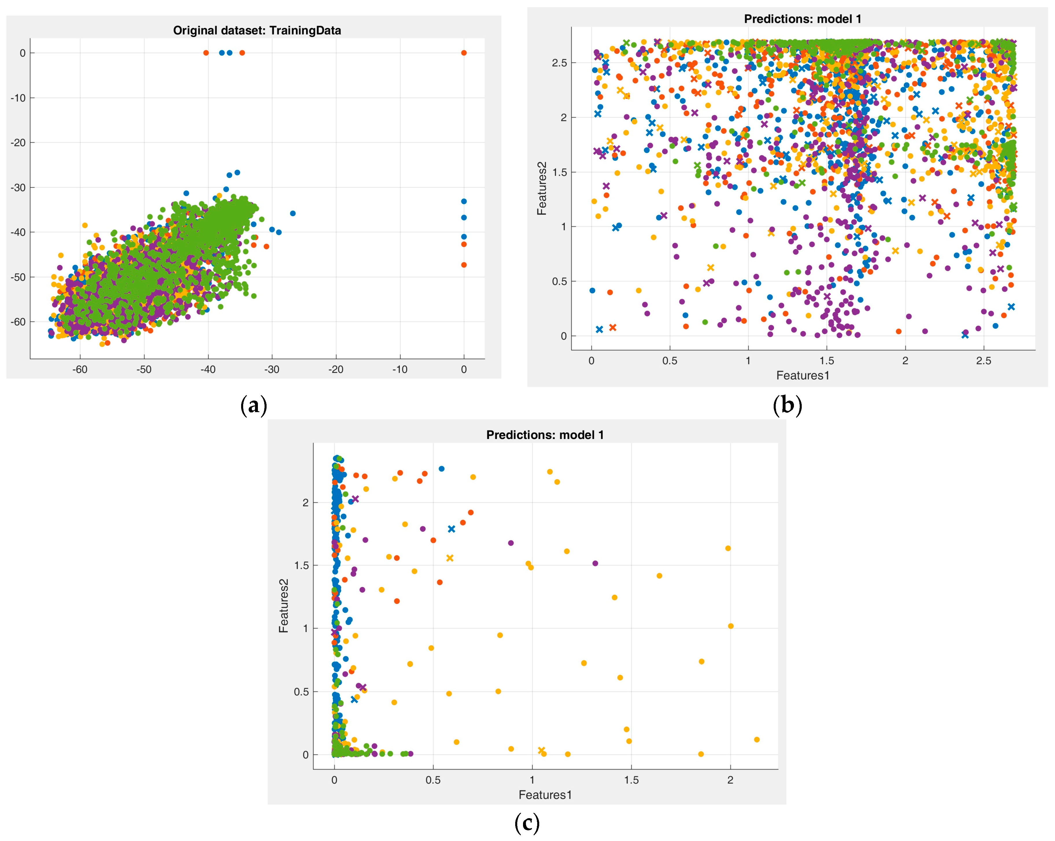
Referring to Figure 5, the data training phase has been shown, where data and features are distributed clearly shows that in case of DWT, the data is spread more across its region in plan, as it represents both lower and higher frequencies on its axes hence better performance evaluation.
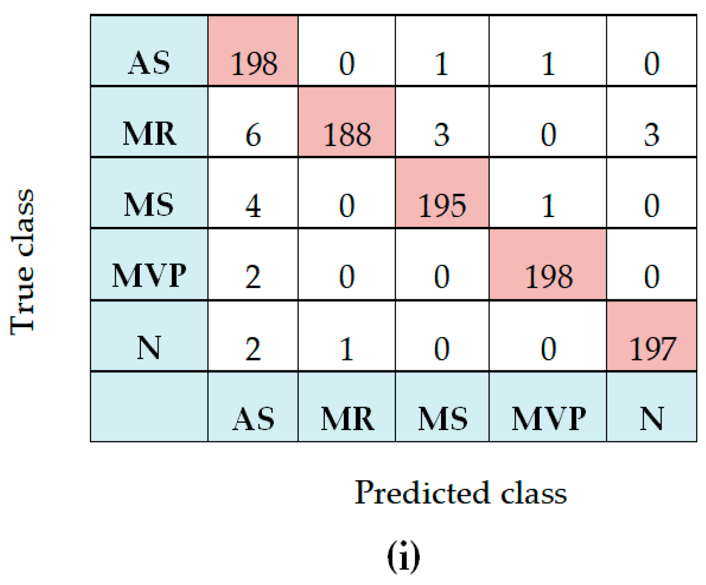
Figure 6 shows confusion matrices for features type and the training model, as explained in the footer section of this figure, a; d; g belongs to MFCCs features, b, e, h belongs to DWT features and c, f, i belongs to combined features (MFCCs plus DWT).
The heart sound signal preprocessing and classification is performed by three different methods and classifiers. In case of any speech and signal processing, study shows that features extracted with wavelets transform have greater performance and when those features are used in combination with MFCCs, the accuracy goes even higher [5,6,25].
5. Results and Discussion
In our experiments we classified our extracted features from heart sound signal database (including normal and abnormal category) using three different classifiers, SVM, DNN and centroid based KNN. Table 2 shows the baseline results obtained using MFCCs features and their corresponding accuracies. In order to improve the accuracy, we found out some optimum values for feature extraction such as sampling frequency and feature vector length on which the resulting accuracies were higher than before and the results are shown in Table 3. For better accuracy, new features (DWT) were taken into consideration for our experiments, after experimenting and training our data with DWT we have achieved results shown in Table 4. We can see from Table 3 and Table 4 that there is improvement in the accuracy but we considered to combine those features together and train using SVM and DNN, after performing experiments and finding some optimal values for sampling frequency, we arrived at the conclusion that we have much better output than using those features separately, and we can see the results from Table 5. Unfortunately DNN couldn’t perform well as compared to SVM and the reason for that is we have very limited amount of data available and we know that DNN requires thousands of files and features for training and classification, so in case if sufficient amount of data were available, DNN could have performed higher than SVM.
The highest accuracy we achieved from those experiments was from fused (combined) features we classified; these combined features have never been used for classification of heart sound signal before. Table 3, Table 4, Table 5 and Table 6 summarizes the output, and classification in terms of accuracy averaged f1 score sensitivity and specificity of our experiment in detail. Several experiments were performed with MFCCs and DWT with variant frequencies, variant Cepstral coefficient and their corresponding changing accuracy was recorded. From our experiments Table 3, Table 4 and Table 5 summarize the last and final results of MFCCs, DWT and combined features (MFCCs and DWT) respectively.
Depending on the size of dataset and type of features in the classification experiment different results can be achieved with variant accuracies. Using fivefold cross validation the evaluation results are achieved as shown in Table 5. It is observed that the overall maximum accuracy of 97.9% (F1 score of 99.7%) has been achieved using combine features of discrete wavelet transform and MFCCs, and training them via SVM classifier. In case of centroid displacement based KNN the highest accuracy achieved is 97.4% (F1 score of 99.2%).
Similarly, in case of DNN, the maximum accuracy of 89.3% has been achieved when we used MFCCs Features combined with DWT features, keeping the parameters for all the features same as mentioned in above paragraph, we trained our deep neural network with features (MFCCs and DWT), in deep neural network we kept batch size of 100, three hidden layers and one output layer and 2000 epochs. In case of DNN too, we can observe from our results table that using combined features of MFCCs and DWT, we can get higher results by efficiently utilizing the information present in the heart sound signal. The improved accuracy is due to usage of completely different domain signals (MFCCs and DWT) together.
6. Conclusions
PCG signals carries information about the functioning of heart valves during heartbeat, hence these signals are very important in diagnosing heart problems at early stage. To detect heart problems with great precision, the new features (MFCCs and DWT) were used and have been proposed in this study to detect 4 types of abnormal heart diseases category and one normal category. The results that have been obtained shows clear performance superiority and can help physicians in the early detection of heart disease during auscultation examination. This work can be greatly improved if the dataset is prepared on a larger scale and also if the data features are managed in a more innovative way, then the performance can be more fruitful. Some new features can also be introduced to asses and analyses heart sound signal more accurately.
Author Contributions
The authors contributed equally to this work. Conceptualization, visualization, writing and preparing the manuscript is done by Y., reviewing, supervision, project administration, validation and funding was done by S.K., Software related work, data creation, project administration was the task of G.Y.S.
Funding
This research was funded by the Ministry of SMEs and Startups (No. S2442956). The APC was funded by Sejong University.
Acknowledgments
This work was supported by the Ministry of SMEs and Startups (No. S2442956), the development of intelligent stethoscope sounds analysis engine and interactive smart stethoscope service platform.
Conflicts of Interest
The authors declare no conflict of interest.
Appendix A
The data was collected from random sources, such as books (Auscultation skills CD, Heart sound made easy) and websites (48 different websites provided the data including Washington, Texas, 3M, and Michigan and so on). After conducting efficient cross check test, we excluded files having extreme noise, data was sampled to 8000 Hz frequency rate and was converted to mono channel, 3 period heart sound signal, data sampling, conversion and editing was done in cool edit software.
References
- Bolea, J.; Laguna, P.; Caiani, E.G.; Almeida, R. Heart rate and ventricular repolarization variabilities interactions modification by microgravity simulation during head-down bed rest test. In Proceedings of the 2013 IEEE 26th International Symposium onComputer-Based Medical Systems (CBMS), Porto, Portugal, 22–23 June 2013; IEEE: New York, NY, USA, 2013; pp. 552–553. [Google Scholar]
- Kwak, C.; Kwon, O.-W. Cardiac disorder classification by heart sound signals using murmur likelihood and hidden markov model state likelihood. IET Signal Process. 2012, 6, 326–334. [Google Scholar] [CrossRef]
- Mondal, A.; Kumar, A.K.; Bhattacharya, P.; Saha, G. Boundary estimation of cardiac events s1 and s2 based on hilbert transform and adaptive thresholding approach. In Proceedings of the 2013 Indian Conference on Medical Informatics and Telemedicine (ICMIT), Kharagpur, India, 28–30 March 2013; IEEE: New York, NY, USA, 2013; pp. 43–47. [Google Scholar]
- Randhawa, S.K.; Singh, M. Classification of heart sound signals using multi-modal features. Procedia Computer Science 2015, 58, 165–171. [Google Scholar] [CrossRef]
- Anusuya, M.; Katti, S. Comparison of different speech feature extraction techniques with and without wavelet transform to kannada speech recognition. Int. J. Comput. Appl. 2011, 26, 19–24. [Google Scholar] [CrossRef]
- Turner, C.; Joseph, A. A wavelet packet and mel-frequency cepstral coefficients-based feature extraction method for speaker identification. Procedia Comput. Sci. 2015, 61, 416–421. [Google Scholar] [CrossRef]
- Thiyagaraja, S.R.; Dantu, R.; Shrestha, P.L.; Chitnis, A.; Thompson, M.A.; Anumandla, P.T.; Sarma, T.; Dantu, S. A novel heart-mobile interface for detection and classification of heart sounds. Biomed. Signal Process. Control 2018, 45, 313–324. [Google Scholar] [CrossRef]
- Wu, J.-B.; Zhou, S.; Wu, Z.; Wu, X.-M. Research on the method of characteristic extraction and classification of phonocardiogram. In Proceedings of the 2012 International Conference on Systems and Informatics (ICSAI), Yantai, China, 19–20 May 2012; IEEE: New York, NY, USA, 2012; pp. 1732–1735. [Google Scholar]
- Maas, A.L.; Qi, P.; Xie, Z.; Hannun, A.Y.; Lengerich, C.T.; Jurafsky, D.; Ng, A.Y. Building dnn acoustic models for large vocabulary speech recognition. Comput. Speech Lang. 2017, 41, 195–213. [Google Scholar] [CrossRef]
- Nanni, L.; Aguiar, R.L.; Costa, Y.M.; Brahnam, S.; Silla, C.N., Jr.; Brattin, R.L.; Zhao, Z. Bird and whale species identification using sound images. IET Comput. Vis. 2017, 12, 178–184. [Google Scholar] [CrossRef]
- Nanni, L.; Costa, Y.M.; Aguiar, R.L.; Silla, C.N., Jr.; Brahnam, S. Ensemble of deep learning, visual and acoustic features for music genre classification. J. New Music Res. 2018, 1–15. [Google Scholar] [CrossRef]
- Nair, A.P.; Krishnan, S.; Saquib, Z. Mfcc based noise reduction in asr using kalman filtering. In Proceedings of the Conference on Advances in Signal Processing (CASP), Pune, India, 9–11 June 2016; IEEE: New York, NY, USA, 2016; pp. 474–478. [Google Scholar]
- Almisreb, A.A.; Abidin, A.F.; Tahir, N.M. Comparison of speech features for arabic phonemes recognition system based malay speaker. In Proceedings of the 2014 IEEE Conference on Systems, Process and Control (ICSPC), Kuala Lumpur, Malaysia, 12–14 December 2014; IEEE: New York, NY, USA, 2014; pp. 79–83. [Google Scholar]
- DeRose, E.J.S.T.D.; Salesin, D.H. Wavelets for computer graphics: A primer part 1 y. Way 1995, 6, 1. [Google Scholar]
- Ghazali, K.H.; Mansor, M.F.; Mustafa, M.M.; Hussain, A. Feature extraction technique using discrete wavelet transform for image classification. In Proceedings of the 5th Student Conference on Research and Development SCOReD 2007, Selangor, Malaysia, 11–12 December 2007; IEEE: New York, NY, USA, 2007; pp. 1–4. [Google Scholar]
- Fahmy, M.M. Palmprint recognition based on mel frequency cepstral coefficients feature extraction. Ain Shams Eng. J. 2010, 1, 39–47. [Google Scholar] [CrossRef]
- Sharma, R.; Kesarwani, A.; Mathur, P.M. A novel compression algorithm using dwt. In Proceedings of the 2014 Annual IEEE India Conference (INDICON), Pune, India, 11–13 December 2014; IEEE: New York, NY, USA, 2014; pp. 1–4. [Google Scholar]
- Li, M.; Chen, W.; Zhang, T. Classification of epilepsy eeg signals using dwt-based envelope analysis and neural network ensemble. Biomed. Signal Process. Control 2017, 31, 357–365. [Google Scholar] [CrossRef]
- Zhong, Y.-C.; Li, F. Model identification study on micro robot mobile in liquid based on support vector machine. In Proceedings of the 3rd IEEE International Conference onNano/Micro Engineered and Molecular Systems, NEMS 2008, Sanya, China, 6–9 January 2008; IEEE: New York, NY, USA, 2008; pp. 55–59. [Google Scholar]
- Lu, P.; Xu, D.-P.; Liu, Y.-B. Study of fault diagnosis model based on multi-class wavelet support vector machines. In Proceedings of the 2005 International Conference on Machine Learning and Cybernetics, Guangzhou, China, 18–21 August 2005; IEEE: New York, NY, USA; pp. 4319–4321. [Google Scholar]
- Yang, K.-H.; Zhao, L.-L. Application of the improved support vector machine on vehicle recognition. In Proceedings of the 2008 International Conference on Machine Learning and Cybernetics, Kunming, China, 12–15 July 2008; IEEE: New York, NY, USA, 2008; pp. 2785–2789. [Google Scholar]
- Chapelle, O.; Vapnik, V.; Bousquet, O.; Mukherjee, S. Choosing multiple parameters for support vector machines. Mach. Learn. 2002, 46, 131–159. [Google Scholar] [CrossRef]
- Yi, H.; Sun, S.; Duan, X.; Chen, Z. A study on deep neural networks framework. In Proceedings of the 2016 IEEE Advanced Information Management, Communicates, Electronic and Automation Control Conference (IMCEC), Xi’an, China, 3–5 October 2016; IEEE: New York, NY, USA, 2016; pp. 1519–1522. [Google Scholar]
- Nguyen, B.P.; Tay, W.-L.; Chui, C.-K. Robust biometric recognition from palm depth images for gloved hands. IEEE Trans. Hum.-Mach. Syst. 2015, 45, 799–804. [Google Scholar] [CrossRef]
- Janse, P.V.; Magre, S.B.; Kurzekar, P.K.; Deshmukh, R. A comparative study between mfcc and dwt feature extraction technique. Int. J. Eng. Res. Technol. 2014, 3, 3124–3127. [Google Scholar]
Figure 1.
(a) A normal heart sound signal; (b) Murmur in systole (MVP); (c) Mitral Regurgitation (MR); (d) Mitral Stenosis (MS); (e) Aortic Stenosis (AS); (f) Spectrum of a PCG signal.
Figure 1.
(a) A normal heart sound signal; (b) Murmur in systole (MVP); (c) Mitral Regurgitation (MR); (d) Mitral Stenosis (MS); (e) Aortic Stenosis (AS); (f) Spectrum of a PCG signal.


Figure 2.
(a) Proposed heart sound signal classification algorithm using SVM; (b) Proposed heart sound signal classification algorithm using DNN.
Figure 2.
(a) Proposed heart sound signal classification algorithm using SVM; (b) Proposed heart sound signal classification algorithm using DNN.

Figure 3.
(a) MFCCs computation; (b) Decomposition tree of wavelets (3rd level).

Figure 4.
(a) Neural network composed of many interrelated neurons; (b) Data collection procedure outline.
Figure 4.
(a) Neural network composed of many interrelated neurons; (b) Data collection procedure outline.

Figure 5.
(a) MFCCs Features data pattern; (b) DWT Features data pattern; (c) DWT plus MFCCs Features data pattern.
Figure 5.
(a) MFCCs Features data pattern; (b) DWT Features data pattern; (c) DWT plus MFCCs Features data pattern.

Figure 6.
(a) Confusion matrix for MFCCs Features and Centroid displacement based KNN classifier; (b) Confusion matrix for DWT Features and Centroid displacement based KNN classifier; (c) Confusion matrix for MFCCs plus DWT Features and Centroid displacement based KNN classifier; (d) Confusion matrix for MFCCs Features and DNN classifier; (e) Confusion matrix for DWT Features and DNN classifier; (f) Confusion matrix for MFCCs plus DWT Features and DNN classifier; (g) Confusion matrix for MFCCs Features and SVM classifier; (h) Confusion matrix for DWT Features and SVM classifier; (i) Confusion matrix for MFCCs plus DWT Features and SVM classifier.


Table 1.
Dataset detail.
| Classes | Number of Samples Per Class | |
|---|---|---|
| Normal | N | 200 |
| Abnormal | AS | 200 |
| MR | 200 | |
| MS | 200 | |
| MVP | 200 | |
| Total | 1000 |
Table 2.
Baseline results with MFCCs features.
| Classifier | Features | Accuracy |
|---|---|---|
| SVM | MFCC | 87.2% |
| DNN | MFCC | 82.3% |
| Centroid displacement base KkNN | MFCC | 72.2% |
Table 3.
Improved Result based on MFCCs Features.
| MFCCs | KNN (Centroid Displacement Based) | SVM | DNN |
|---|---|---|---|
| Accuracy | 80.2% | 91.6% | 86.5% |
| Average F1 Score | 92.5% | 86.0% | 96.9% |
Table 4.
Result based on DWT Features.
| DWT | KNN (Centroid Displacement Based) | SVM | DNN |
|---|---|---|---|
| Accuracy | 91.8% | 92.3% | 87.8% |
| Average F1 Score | 98.3% | 99.1% | 95.6% |
Table 5.
Result based on MFCCs and DWT Features.
| MFCCs + DWT | KNN (Centroid Displacement Based) | SVM | DNN |
|---|---|---|---|
| Accuracy | 97.4% | 97.9% | 92.1% |
| Average F1 Score | 99.2% | 99.7% | 98.3% |
Table 6.
Sensitivity and Specificity calculated for each classifier performance based on the Figure 6 confusion matrix.
Table 6.
Sensitivity and Specificity calculated for each classifier performance based on the Figure 6 confusion matrix.
| Classifiers | Features | Sensitivity | Specificity |
|---|---|---|---|
| Centroid displacement based KNN | MFCCs | 81.98% | 93.5% |
| DWT | 92.0% | 97.9% | |
| MFCCs + DWT | 97.6% | 98.8% | |
| DNN | MFCCs | 86.8% | 95.1% |
| DWT | 91.6% | 97.4% | |
| MFCCs + DWT | 94.5% | 98.2% | |
| SVM | MFCCs | 87.3% | 96.6% |
| DWT | 92.3% | 98.4% | |
| MFCCs + DWT | 98.2% | 99.4% |
© 2018 by the authors. Licensee MDPI, Basel, Switzerland. This article is an open access article distributed under the terms and conditions of the Creative Commons Attribution (CC BY) license (http://creativecommons.org/licenses/by/4.0/).
Share and Cite
MDPI and ACS Style
Yaseen; Son, G.-Y.; Kwon, S. Classification of Heart Sound Signal Using Multiple Features. Appl. Sci. 2018, 8, 2344. https://0-doi-org.brum.beds.ac.uk/10.3390/app8122344
AMA Style
Yaseen, Son G-Y, Kwon S. Classification of Heart Sound Signal Using Multiple Features. Applied Sciences. 2018; 8(12):2344. https://0-doi-org.brum.beds.ac.uk/10.3390/app8122344
Chicago/Turabian StyleYaseen, Gui-Young Son, and Soonil Kwon. 2018. "Classification of Heart Sound Signal Using Multiple Features" Applied Sciences 8, no. 12: 2344. https://0-doi-org.brum.beds.ac.uk/10.3390/app8122344
Note that from the first issue of 2016, this journal uses article numbers instead of page numbers. See further details here.