Recognition of Acoustic Signals of Commutator Motors


Department of Automatic Control and Robotics, Faculty of Electrical Engineering, Automatics, Computer Science and Biomedical Engineering, AGH University of Science and Technology, al. A. Mickiewicza 30, 30-059 Kraków, Poland
Appl. Sci. 2018, 8(12), 2630; https://0-doi-org.brum.beds.ac.uk/10.3390/app8122630
Submission received: 15 November 2018
/
Revised: 11 December 2018
/
Accepted: 12 December 2018
/
Published: 15 December 2018
(This article belongs to the Special Issue Fault Diagnosis of Rotating Machine)
Abstract
:Most faults can stop a motor, and time is lost in fixing the damaged motor. This is a reason why it is essential to develop fault-detection methods. This paper describes the acoustic-based fault detection of two commutator motors: the commutator motor of an electric impact drill and the commutator motor of a blender. Acoustic signals were recorded by a smartphone. Five states of the electric impact drill and three states of the blender were analysed: for the electric impact drill, these states were healthy, damaged gear train, faulty fan with five broken rotor blades, faulty fan with 10 broken rotor blades, and shifted brush (motor off); for the blender, these states were healthy, faulty fan with two broken rotor blades, and faulty fan with five broken rotor blades. A feature extraction method, MSAF-RATIO-27-MULTIEXPANDED-4-GROUPS (Method of Selection of Amplitudes of Frequency Ratio of 27% Multiexpanded 4 Groups), was developed and used for the computation of feature vectors. The nearest mean (NM) and support vector machine (SVM) classifiers were used for data classification. Analysis of the recognition of acoustic signals was carried out. The analysed value of TEEID (the total efficiency of recognition of the electric impact drill) was equal to 96% for the NM classifier and 88.8% for SVM. The analysed value of TEB (the total efficiency of recognition of the blender) was equal to 100% for the NM classifier and 94.11% for SVM.
Keywords:
electrical machine; classification; mechanical fault; detection; analysis; sound; commutator motors1. Introduction
Commutator motors (CMs) are the most frequently used electrical motors for devices used at home, for example, electric impact drills, angle grinders, cordless drills, hair dryers, blenders, etc. CMs are also used in the energy industry, material industry, construction industry, mining industry, transport industry, and by construction and renovation companies. Sometimes, faults of devices can happen. An undetected fault can lead to the damage of the whole device. Frequent faults of commutator motors are: bearing faults, damaged gears, damaged teeth, short-circuits, and damaged electric motor brushes. Bearings hold the shaft of the CM, but they wear out after years of use. Most of these faults can stop the motor. Then, there is a loss of time associated with fixing the damaged motor. It is essential for industrial motors. A production line (consisting of motors) can be stopped for a longer time for repair.
The above constitutes an essential reason for developing fault-detection methods. Diagnostic methods can use various signals, for example: ultrasound, acoustic signals, current signals, magnetic signals, vibration, video images, and thermal images. There is also the possibility of using oil analysis. Ultrasound is used for detecting faults of motors, pumps, and bearings [1,2,3,4]. However, the cost of an ultrasound generator is about $1000. The analysis of acoustic emissions (in the range 30–16,000 Hz) is noninvasive and low-cost [5,6,7,8,9,10,11,12]; however, its main disadvantages are the appearance of background noises and reflected sounds. The analysis of thermal images is also a common diagnostic technique [13,14,15], which is used for electrical faults such as shorted coils and broken bars of the motor. The analysis of electric currents is also used for the fault diagnosis of motors [16,17,18,19,20,21]. Similarly to the analysis of thermal images, it can be used for electrical faults. Vibration analysis is often used for the condition monitoring of motors [22,23,24,25,26,27,28]. Vibration analysis can detect many types of faults, such as rotor and stator faults, mechanical faults, gear faults, cracks, bearing faults, damaged teeth of sprockets, etc. Moreover, a vibration signal is measured immediately.
This paper deals with the fault detection of an electric impact drill and blender using a smartphone. Considering that the electric impact drill and blender consisted of commutator motors and other mechanical parts such as gears, sprockets, etc., five states of the electric impact drill were analysed: healthy (Figure 1), with a damaged gear train (Figure 2), with a faulty fan with five broken rotor blades (Figure 3), with a faulty fan with 10 broken rotor blades (Figure 4), and with a shifted brush (motor off) (Figure 5); and three states of the blender were analysed: healthy (Figure 6), with a faulty fan with 2 broken rotor blades (Figure 7), and with a faulty fan with 5 broken rotor blades (Figure 8).
The developed approach used a smartphone as the measuring device. Acoustic signals were recorded by the smartphone. Next, the signals were processed by a method of amplitude normalization, MSAF-RATIO-27-MULTIEXPANDED-4-GROUPS (Method of Selection of Amplitudes of Frequency Ratio 27% Multiexpanded 4 Groups—described more in detail in Section 2.1) and nearest mean and SVM classifiers. The results of the fault detection for the electric impact drill and blender are presented in Section 3.
2. Proposed Fault Detection Approach Using a Smartphone and Acoustic Signals
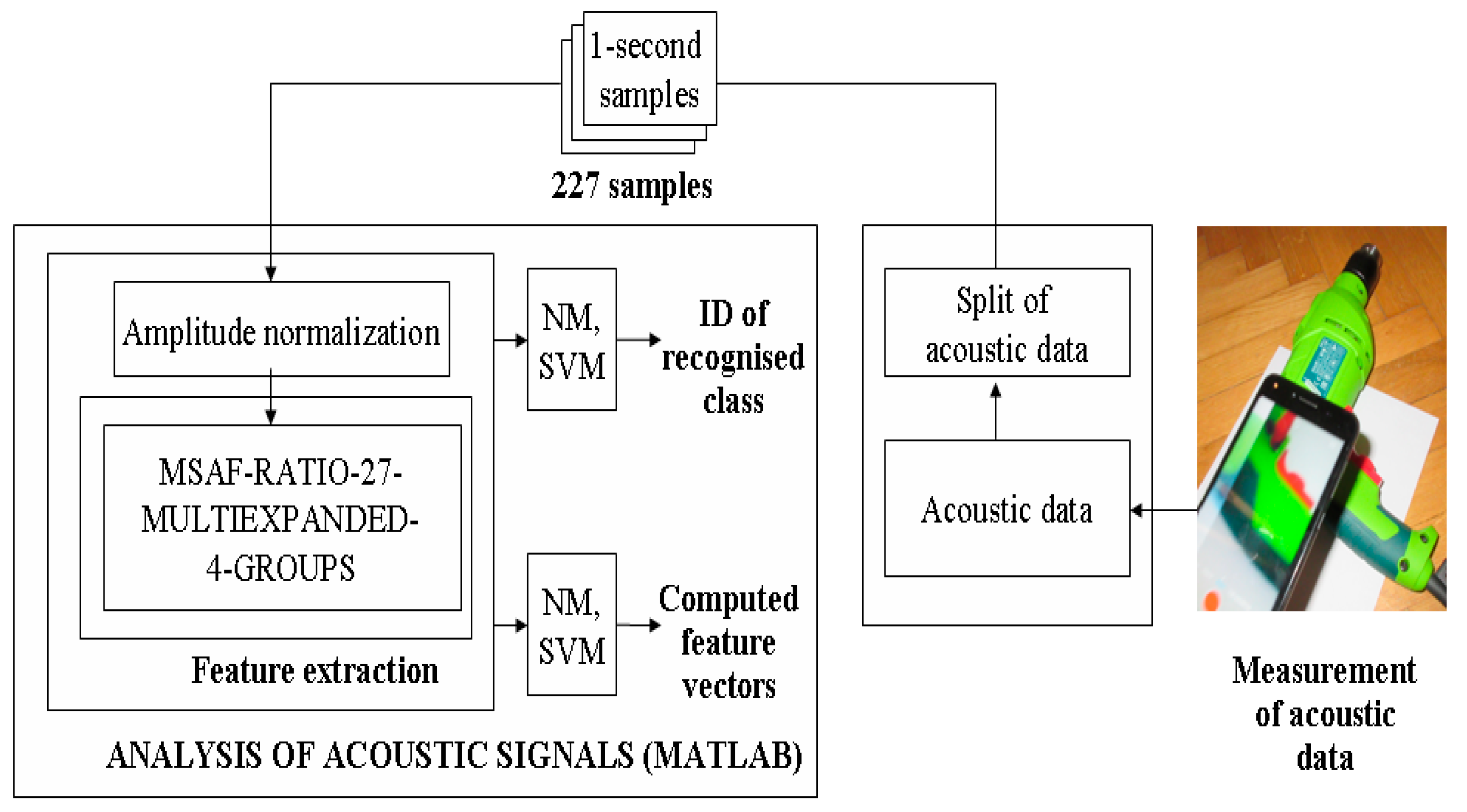
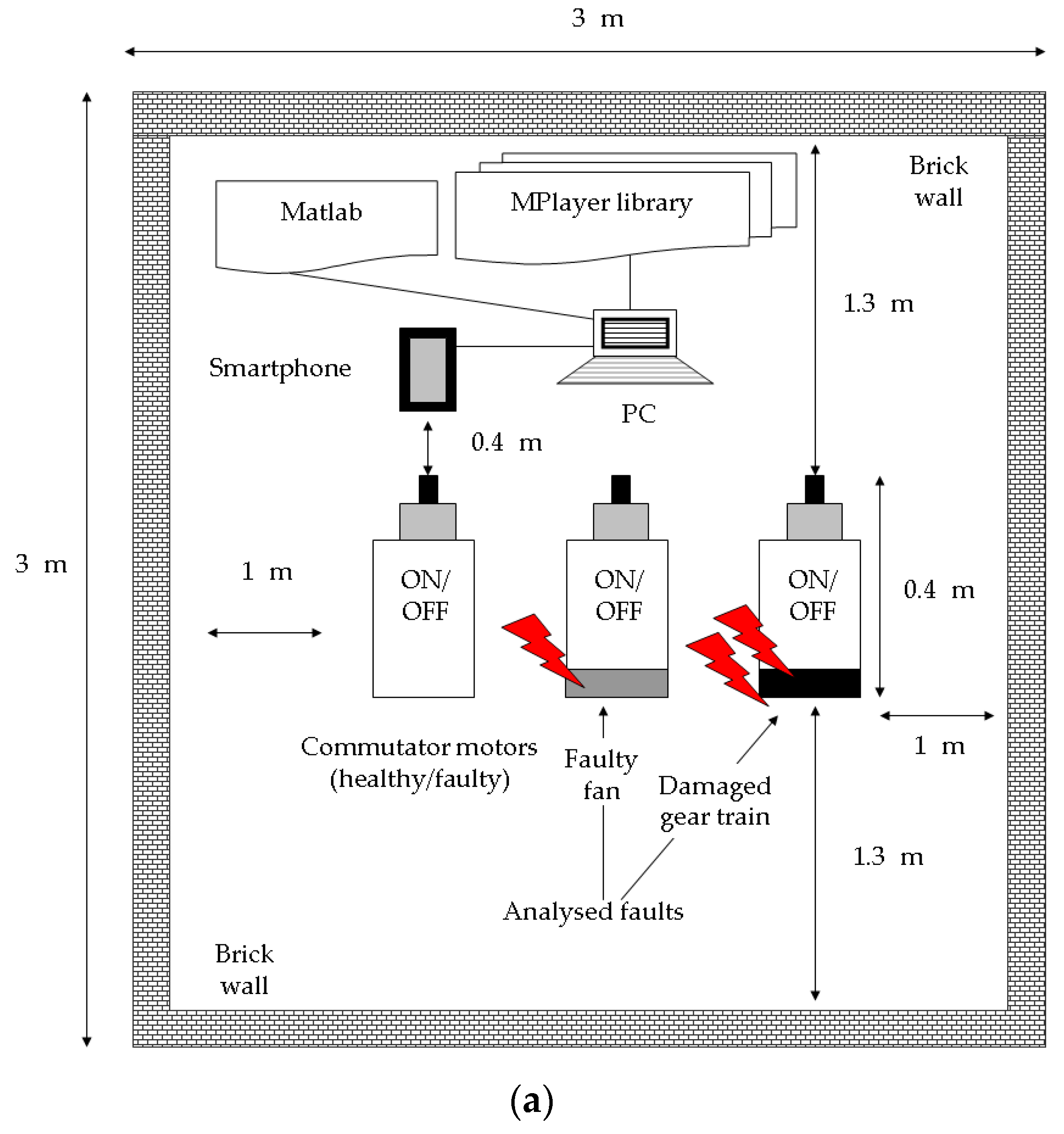
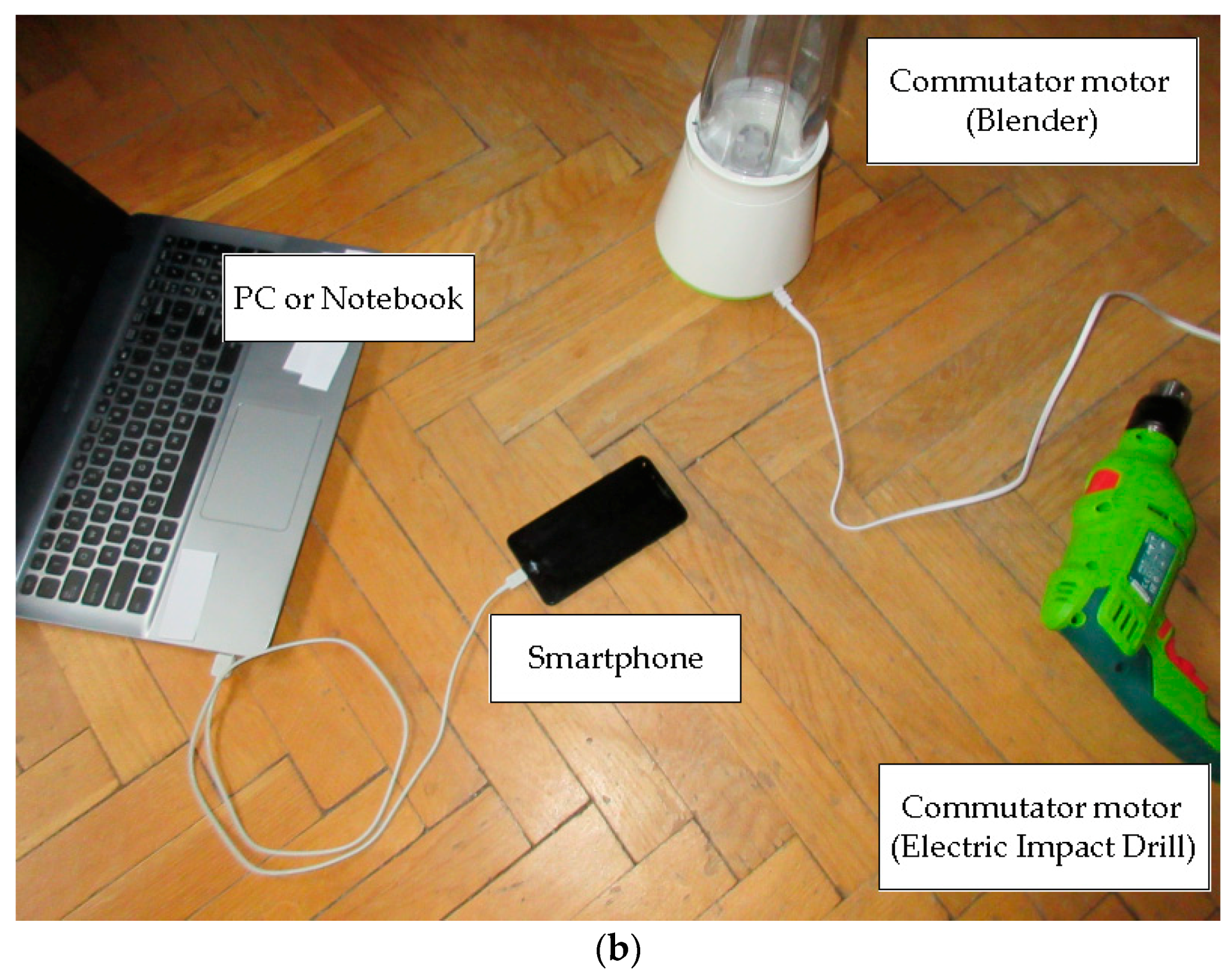
The smartphone can record acoustic signals (parameters of a microphone: frequency response: 30–16,000 Hz, sensitivity: −42 dB). The smartphone was positioned above the electric impact drill/blender (0.4 m above the device). Next, the recorded acoustic signals were converted into acoustic data using ‘MPlayer library—The Movie Player’. Obtained acoustic data (single channel, 44.1-kHz sampling frequency) were processed by signal processing methods: splitting the soundtrack into 1-s samples, a method of amplitude normalization, MSAF-RATIO-27-MULTIEXPANDED-4-GROUPS, the nearest mean classifier, and the SVM classifier. A flowchart of the proposed fault-detection approach is presented in Figure 9. An experimental setup of the measurements using the smartphone is presented in Figure 10a,b.
2.1. MSAF-RATIO-27-MULTIEXPANDED-4-GROUPS
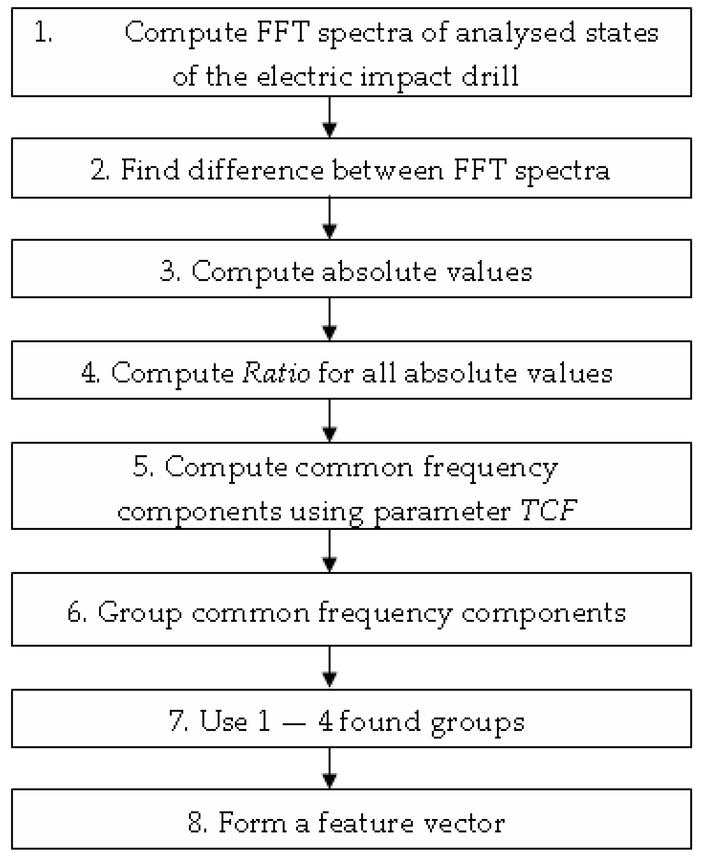
It is difficult to see changes of signals in the time domain; this is a reason to use the frequency domain. The MSAF-RATIO-27-MULTIEXPANDED-4-GROUPS (Method of Selection of Amplitudes of Frequency Ratio 27% Multiexpanded 4 Groups) method computed the FFT (Fast Fourier Transform) spectra. Next, the method computed feature vectors of the analysed states of the electric impact drill. The method used the differences of the FFT spectra. The proposed method used the following steps:
- Compute the FFT spectra of the analysed states of the electric impact drill. Each FFT spectrum had 16,384 values. These values formed 16,384 elements of the vector. Vectors were denoted as follows: healthy electric impact drill—hd = [hd1, hd2, …, hd16,384], electric impact drill with damaged gear train—ddgt = [ddgt1, ddgt2, …, ddgt16,384], electric impact drill with a faulty fan (5 broken rotor blades)—dfive = [dfive1, dfive2, …, dfive16,384], electric impact drill with a faulty fan (10 broken rotor blades)—dten = [dten1, dten2, …, dten16,384],
- Find difference between the FFT spectra: hd − ddgt, hd − dfive, hd − dten, ddgt − dfive, ddgt − dten, dfive − dten.
- Compute absolute values: |hd − ddgt|, |hd − dfive|, |hd − dten|, |ddgt − dfive|, |ddgt − dten|, |dfive − dten|.
- Compute Ratio from Equation (1) for all absolute values:where MaxAV is the maximum absolute value of the difference between FFT spectra, AVi is the absolute value of the difference between FFT spectra with index i, and Ratio is the threshold of the difference between FFT spectra. The RATIO-27 means that 27% of the maximum absolute value of the difference between FFT spectra was the threshold. First, the ratio is defined, and next, it is fixed to a specific threshold. All frequency components larger than the threshold were used for the further steps of processing.Ratio = (100%)AVi/MaxAV
- Compute common frequency components using the parameter TCF (Threshold of common frequency components) = (number of required common frequency components)/(number of all differences). An example of using TCF is presented as follows. There are the following differences of the FFT spectra: |hd − ddgt|, |hd − dfive|, |hd − dten|, |ddgt − dfive|, |ddgt − dten|, |dfive − dten|. Frequency components of 100 and 150 Hz are selected 3 times for |hd − ddgt|. Frequency components of 100 and 200 Hz are selected 3 times for |hd − dfive|. Frequency components of 100 and 300 Hz are selected 3 times for |hd − dten|. Frequency components of 400 and 450 Hz are selected 3 times for |ddgt − dfive|. Frequency components of 400 and 500 Hz are selected 3 times for |ddgt − dten|. Frequency components of 400 and 600 Hz are selected 3 times for |dfive − dten|. It can be noticed that the best frequency components are 100 and 400 Hz, being found 9 times (if TCF = 9/18 = 0.5, it assumes, that 9 required common frequency components are set and there are 18 differences between 4 states, it assumes there are 3 training sets, then it will have 18 differences). The MSAF-RATIO-27-MULTIEXPANDED-4-GROUPS finds none of the frequency components (if TCF = 11/18 = 0.6111 − 11 required common frequency components/18 differences).
- Group the common frequency components. The MSAF-RATIO-27-MULTIEXPANDED-4-GROUPS used 1–4 groups of the best common frequency components. In the mentioned example, the best group had the common frequency components of 100 and 400 Hz.
- Use 1–4 of the found groups.
- Form a feature vector.
A flowchart of the proposed method of feature extraction, MSAF-RATIO-27-MULTIEXPANDED-4-GROUPS, is shown in Figure 11.
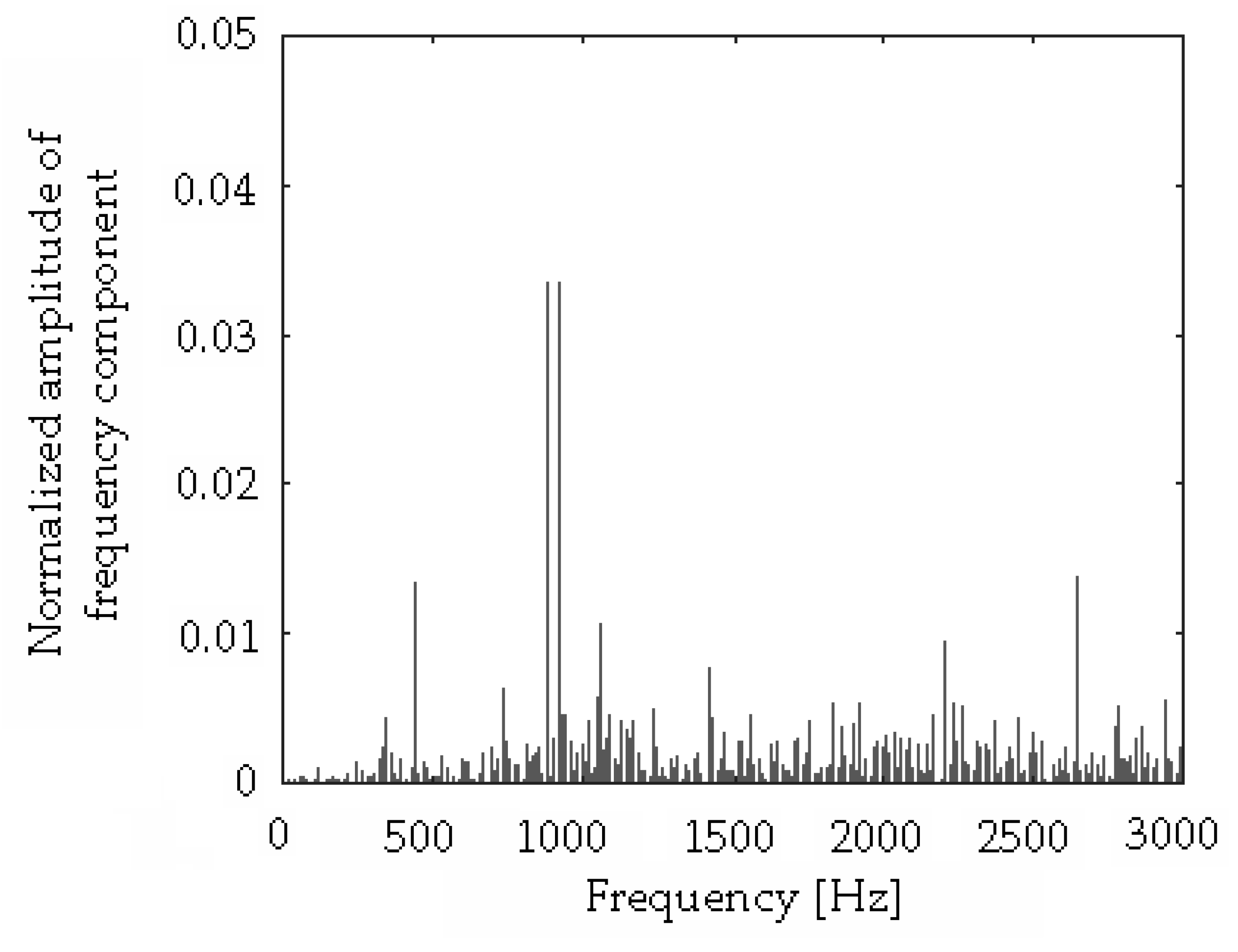
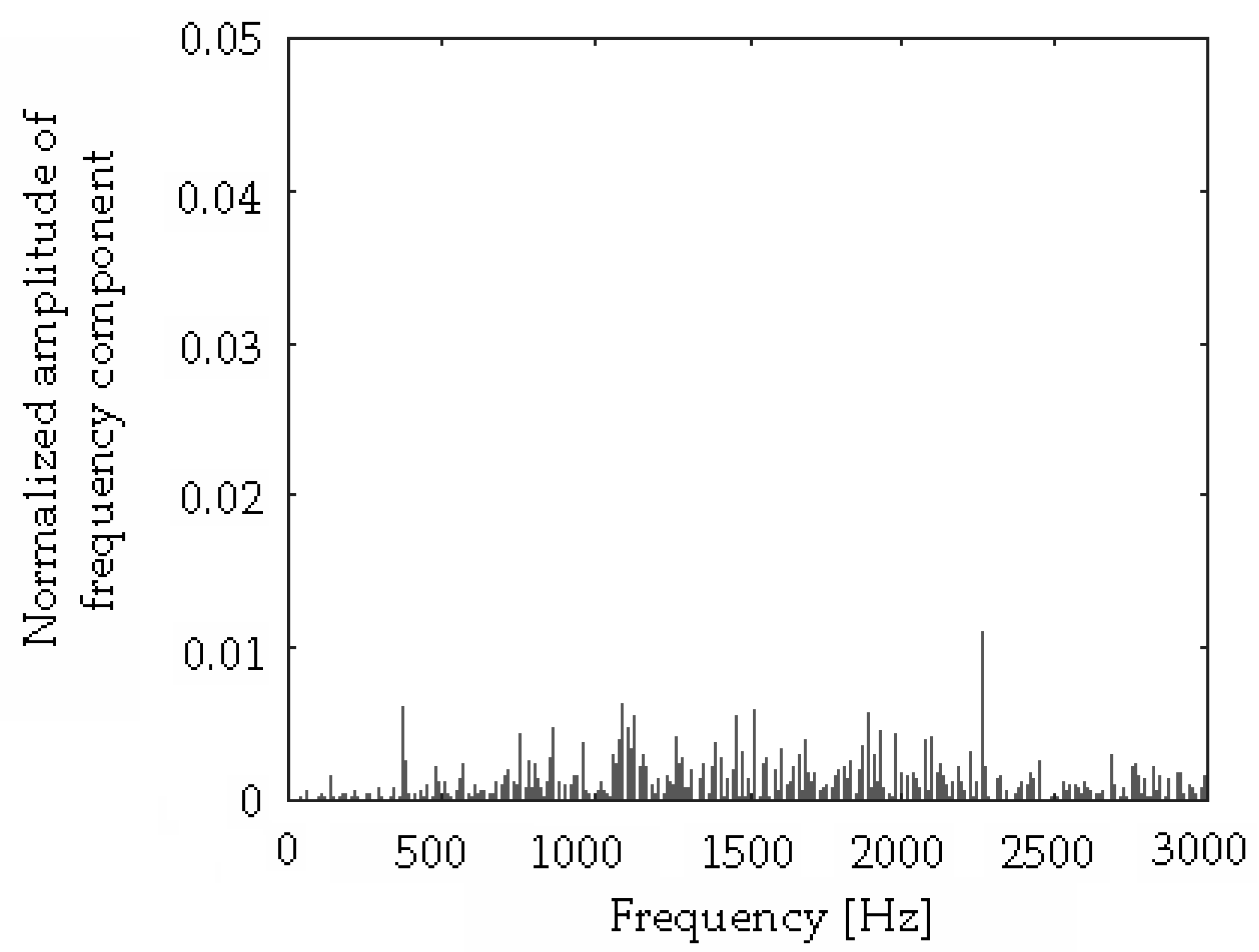
Computed differences between the FFT spectra of the analysed states of the electric impact drill (rotor speed: 3000 rpm) are shown in Figure 12, Figure 13, Figure 14, Figure 15, Figure 16 and Figure 17. Next, we can select the best frequency components for all differences.
The analysed states are compared with each other. If there are 3 states, 3 differences are analysed for 1 training set. If there are 4 states, 6 differences are analysed for 1 training set. If there are 5 states, 10 differences are analysed for 1 training set. If there are 5 states, 30 differences are analysed for 3 training sets. The MSAF-RATIO-27-MULTIEXPANDED-4-GROUPS method computed 12 common frequency components for the electric impact drill: 355, 356, 371, 433, 707, 709, 865, 866, 1108, 1110, 1112, and 1297 Hz for TCF = 0.25 (6/24). The computed frequency components were used for feature vectors (see Table 1, Table 2, Table 3, Table 4 and Table 5 and Figure 18, Figure 19, Figure 20, Figure 21 and Figure 22).
The MSAF-RATIO-27-MULTIEXPANDED-4-GROUPS method computed 12 common frequency components of the blender: 280, 281, 292, 293, 295, 296, 479, 480, 1915, 1916, 2383, and 2479 Hz for TCF = 0.222 (4/18). The computed frequency components were used for feature vectors (Table 6, Table 7 and Table 8) (Figure 23, Figure 24 and Figure 25).
2.2. NM Classifier
To classify feature vectors, the NM classifier was used. It is a well-known classifier used for various applications (similar to the nearest neighbour classifier and k-means clustering) [29,30,31,32,33,34,35,36]. It used an averaged feature vector. The averaged feature vector was the arithmetic average of the training feature vectors of one class. For example, for 5 classes, there are 5 vectors. Next, the averaged feature vector was compared with the test feature vector using the Manhattan distance (Equation (2)).
where MD(a − hd) is the Manhattan distance for vectors a and hd, where the test vector a = [a264, a265, a276, a322, a526, a527, a643, a644, a824, a825, a827, a964] and the averaged vector hd = [hd264, hd265, hd276, hd322, hd526, hd527, hd643, hd644, hd824, hd825, hd827, hd964].
The NM classifier performed Equation (2) for all feature vectors: |a − hd|, |a − ddgt|, |a − dfive|, |a − dten|. The nearest distance between vectors was essential for making decisions about the recognised class. For example, if |a − hd| is the nearest distance, then the class “healthy electric impact drill” will be recognised.
There are 2 recordings of the electric impact drill in the presented approach. The first recording was split into training samples. The second recording was split into test samples. The MSAF-RATIO-27-MULTIEXPANDED-4-GROUPS method used the training samples. Next, it computed the common frequency components (in the analysed case, it was 12 common frequency components; please see Section 2). The number of common frequency components depended on the analysed signals. Equation (2) uses the unknown test vector “a” and the known training vector “hd”. Each new recorded test sample is compared with the “training set” (all averaged feature vector). Assuming a signal for a new drill is acquired; next, it is compared with all states in the training set. Moreover, there is also the possibility of adding new training samples and new type of motors to the training set.
2.3. SVM Classifier
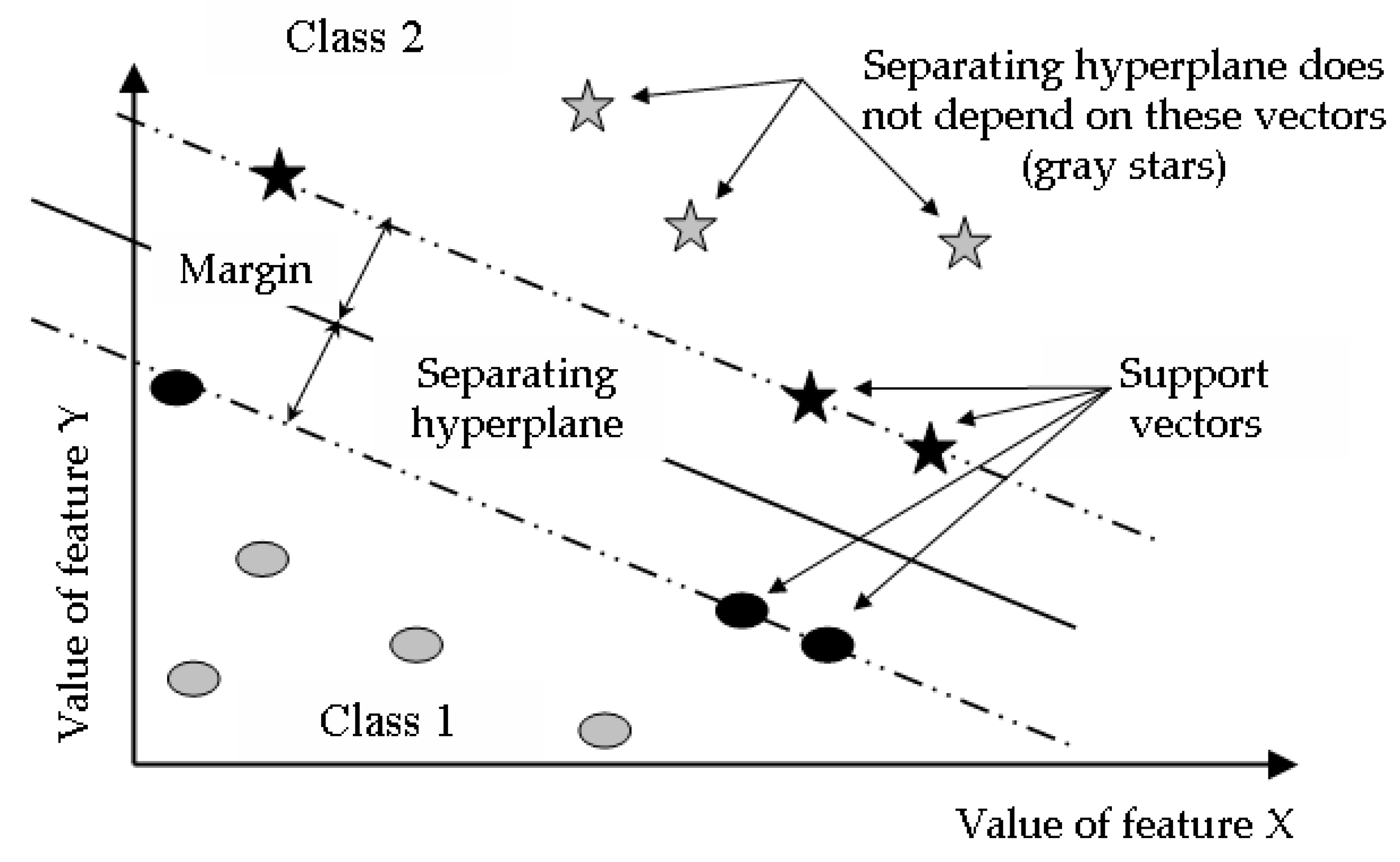
The second method of classification of the processed computed feature vectors (12 dimensions/features in the presented analysis) was using the SVM (support vector machine) classifier [37]. It was the supervised classification method. The SVM used a separating hyperplane. The method computed the separating hyperplane which categorised the unknown test feature vectors. Two classes of feature vectors could be separated by many hyperplanes. The objective of the SVM classifier was to compute the separating hyperplane that had the maximum margin [37]. The margin was the maximum distance between the analysed feature vectors. The hyperplane was a boundary between the analysed classes. It helped categorise the feature vectors. Feature vectors could be attributed to two classes (for example, healthy electric impact drill and electric impact drill with damaged gear train). This depended on the features of the vector and the location of the hyperplane.
The hyperplane was a line if the number of elements of feature vectors was equal to two. The hyperplane was a two-dimensional plane if the number of elements of feature vectors was equal to three.
Computed support vectors were the feature vectors. Support vectors were close to the hyperplane. The SVM model used support vectors to compute the position of the hyperplane. Distances between support vectors and the hyperplane were essential for the proper building of the SVM model (Figure 26).
3. Results of the Fault Detection of the Analysed Commutator Motors
Measurements of the acoustic signals of the analysed commutator motors (the commutator motor of the electric impact drill and the commutator motor of the blender) were conducted in a workshop. The analysed devices were operational, except for the electric impact drill with a shifted brush (motor off). The author measured and analysed five states of the electric impact drill: healthy, with damaged gear train, with a faulty fan with five broken rotor blades, with a faulty fan with 10 broken rotor blades, and with a shifted brush (motor off). Each electric impact drill had a commutator motor and had PEID = 500 W, REID = 3000 rpm, VEID = 230 V, fEID = 50 Hz, and MEID = 1.84 kg, where MEID—weight of the electric impact drill, PEID—rated power of the electric impact drill, REID—rotation speed of the electric impact drill, VEID—supply voltage of the electric impact drill, and fEID—current frequency of the electric impact drill. The author measured and analysed three states of the blender: healthy, with a faulty fan with two broken rotor blades, and with a faulty fan with 5 broken rotor blades. Each blender had a commutator motor and had PB = 300 W, RB = 10,000 rpm, VB = 230 V, and fB = 50 Hz, MB = 1.75 kg, where MB—weight of the blender, PB—rated power of the blender, RB—rotation speed of the blender, VB—supply voltage of the blender, and fB—current frequency of the blender.
To compute patterns, 20 one-second training samples of the electric impact drill and 18 one-second training samples of the blender were analysed. To analyse the proposed approach (please see Section 2), 125 one-second test samples of the electric impact drill and 102 one-second test samples of the blender were analysed. Acoustic data of the analysed commutator motors were evaluated by Equation (3). It defined the efficiency of recognition of the electric impact drill/blender (EEID):
where EEID—the efficiency of recognition of the electric impact drill/blender for the selected type of acoustic signal, NEID—the number of test samples of the electric impact drill/blender tested properly for the selected type of acoustic signal, and NAEID—the number of all test samples of the electric impact drill/blender for the selected type of acoustic signal.
The total efficiency of recognition of the electric impact drill (TEEID) was used to evaluate the EEID of all analysed acoustic signals of the electric impact drill. TEEID was expressed as Equation (4):
where TEEID—the total efficiency of recognition of the electric impact drill for the five selected types of acoustic signals, EEID1—the efficiency of recognition of the healthy electric impact drill, EEID2—the efficiency of recognition of the electric impact drill with a damaged gear train, EEID3—the efficiency of recognition of the electric impact drill with a faulty fan (five broken rotor blades), EEID4—the efficiency of recognition of the electric impact drill with a faulty fan (10 broken rotor blades), and EEID5—the efficiency of recognition of the electric impact drill with a shifted brush (motor off).
The total efficiency of recognition of the blender (TEB) was expressed as Equation (5):
where TEB—the total efficiency of recognition of the blender for three selected types of acoustic signals, EEID−B1—the efficiency of recognition of the healthy blender, EEID−B2—the efficiency of recognition of the blender with a faulty fan (two broken rotor blades), EEID−B3—the efficiency of recognition of the blender with a faulty fan (five broken rotor blades).
Computed TEEID and EEID values are shown in Table 9 and Table 10. The analysis of the acoustic signals of the electric impact drill using the MSAF-RATIO-27-MULTIEXPANDED-4-GROUPS method (12 analysed frequency components) and the NM was carried out (see Table 9).
The analysis of the acoustic signals of the electric impact drill using the MSAF-RATIO-27-MULTIEXPANDED-4-GROUPS method (12 analysed frequency components) and SVM was also carried out (see Table 10).
The computed results of the analysis of the electric impact drill were good (EEID = 84–100% and TEEID = 96%) for the NM classifier. The computed results of the analysis of the electric impact drill were the following: EEID = 72–100% and TEEID = 88.8% for the SVM classifier. The MSAF-RATIO-27-MULTIEXPANDED-4-GROUPS method used 12 frequency components of the acoustic signals of the electric impact drill.
The analysis of the acoustic signals of the blender using the MSAF-RATIO-27-MULTIEXPANDED-4-GROUPS method (12 analysed frequency components) and the NM was carried out (see Table 11).
The analysis of the acoustic signals of the blender using the MSAF-RATIO-27-MULTIEXPANDED-4-GROUPS method (12 analysed frequency components) and SVM was also carried out (Table 12).
The computed results of the analysis of the blender were good (EEID = 100% and TEB = 100%) for the NM classifier. The computed results of the analysis of the blender were the following: EEID = 82–100% and TEB = 94.11% for the SVM classifier. The MSAF-RATIO-27-MULTIEXPANDED-4-GROUPS method used 12 frequency components of the acoustic signals of the blender.
4. Discussion
The dependency of performance on the acoustic sensor was significant. The results of recognition depended on the training samples. If the training samples are measured by a specific type of microphone, then new test samples should be also measured by the same type of microphone. Frequency components can be different for different microphones, but the results should be similar.
Another point is the detection of a new, unknown fault. If there is an unknown fault of the commutator motor, then it will be classified as the nearest neighbour (the nearest spectrum of frequency). For example, if there is an acoustic signal of an aircraft, it will be classified as unknown (for example, the class ‘unknown’ includes the sounds of cars, trains, and aircrafts).
The proposed acoustic-based fault detection with variant selection of methods of recognition was based on the difference of FFT spectra (with normalized amplitude). The analysed differences were not big. The results of the recognition of acoustic signals (see Table 9, Table 10, Table 11 and Table 12) showed that the NM classifier was better than the SVM classifier. The nearest neighbour classifier and the nearest mean classifier are based on distance metrics. Distance metrics were very good for the classification of nonlinearly separable data and linearly separable data. In this paper, the SVM classifier used a linear function, the LSVM (linear SVM), which can classify linearly separable data.
5. Summary and Conclusions
The article presented a means of acoustic-based fault detection with variant selection of methods of recognition for two commutator motors: the commutator motor of an electric impact drill and the commutator motor of a blender. Five states of the electric impact drill were analysed: healthy, with a damaged gear train, with a faulty fan with 5 broken rotor blades, with a faulty fan with 10 broken rotor blades, and with a shifted brush (motor off). Three states of the blender were analysed: healthy, with a faulty fan with 2 broken rotor blades, and with a faulty fan with 5 broken rotor blades.
The MSAF-RATIO-27-MULTIEXPANDED-4-GROUPS method was used for the computation of feature vectors. The NM and SVM classifiers were used for data classification.
The computed results of analysis of the electric impact drill were good, with EEID = 84–100% and TEEID = 96% for the NM classifier. The computed results of analysis of the electric impact drill were EEID = 72–100% and TEEID = 88.8% for the SVM classifier. The computed results of analysis of the blender were very good, with EEID = 100% and TEB = 100% for the NM classifier. The computed results of analysis of the blender were EEID = 82–100% and TEB = 94.11% for the SVM classifier.
The proposed approach did not have a high cost. An ordinary computer and an ordinary smartphone cost about $600. The proposed solution can be used in other applications, such as the fault detection of angle grinders, cordless drills, hair dryers, various types of rotating machines, etc. The proposed approach can find applications in the energy industry, material industry, construction industry, mining industry, transport industry, and for construction and renovation companies. However, there were disadvantages of the proposed analysis: the appearance of background noises and reflected sounds.
The proposed approach can be developed in the future. Acoustic signals of various types of rotating machines can be measured and analysed. Acoustic signals can be measured by many types of microphones or acoustic cameras. There is also the possibility of adding diagnostic signals, such as vibrations or thermal images. To achieve a higher recognition efficiency, new feature extraction and classification methods can be analysed.
Funding
This research was funded by the AGH University of Science and Technology, grant no. 11.11.120.714.
Acknowledgments
This work has been supported by the AGH University of Science and Technology, grant no. 11.11.120.714. The author thanks the unknown reviewers for their valuable suggestions.
Conflicts of Interest
The author declares no conflict of interest.
References
- Heidari, M. Combined Diagnosis of PD Based on the Multidimensional Parameters. Model. Simul. Eng. 2016, 2016, UNSP 5949140. [Google Scholar] [CrossRef]
- Munoz, C.Q.G.; Jimenez, A.A.; Marquez, F.P.G. Wavelet transforms and pattern recognition on ultrasonic guides waves for frozen surface state diagnosis. Renew. Energy 2018, 116, 42–54. [Google Scholar] [CrossRef]
- Chen, X.G.; Liu, D.; Xu, G.H.; Jiang, K.S.; Liang, L. Application of Wavelet Packet Entropy Flow Manifold Learning in Bearing Factory Inspection Using the Ultrasonic Technique. Sensors 2015, 15, 341–351. [Google Scholar] [CrossRef] [PubMed]
- Rezaei, A.; Dadouche, A.; Wickramasinghe, V.; Dmochowski, W. A Comparison Study between Acoustic Sensors for Bearing Fault Detection under Different Speed and Load Using a Variety of Signal Processing Techniques. Tribol. Lubr. Technol. 2014, 70, 77–86. [Google Scholar] [CrossRef]
- Juengert, A. Damage Detection in wind turbine blades using two different acoustic techniques. NDT.net e-J. Nondestruct. Test. 2008. [Google Scholar]
- Zhang, D.C.; Entezami, M.; Stewart, E.; Roberts, C.; Yu, D.J. Adaptive fault feature extraction from wayside acoustic signals from train bearings. J. Sound Vib. 2018, 425, 221–238. [Google Scholar] [CrossRef]
- Omoregbee, H.O.; Heyns, P.S. Fault detection in roller bearing operating at low speed and varying loads using Bayesian robust new hidden Markov model. J. Mech. Sci. Technol. 2018, 32, 4025–4036. [Google Scholar] [CrossRef]
- Elforjani, M.; Shanbr, S. Prognosis of Bearing Acoustic Emission Signals Using Supervised Machine Learning. IEEE Trans. Ind. Electron. 2018, 65, 5864–5871. [Google Scholar] [CrossRef]
- Vaimann, T.; Sobra, J.; Belahcen, A.; Rassolkin, A.; Rolak, M.; Kallaste, A. Induction machine fault detection using smartphone recorded audible noise. IET Sci. Meas. Technol. 2018, 12, 554–560. [Google Scholar] [CrossRef]
- Vanraj Singh, R.; Dhami, S.S.; Pabla, B.S. Development of low-cost non-contact structural health monitoring system for rotating machinery. R. Soc. Open Sci. 2018, 5, 172430. [Google Scholar] [CrossRef]
- Glowacz, A. Acoustic-based fault diagnosis of commutator motor. Electronics 2018, 7, 299. [Google Scholar] [CrossRef]
- Gholamrezaei, S.; Alirezaee, S.; Ahmadi, A.; Ahmadi, M.; Erfani, S. Sound Target Localization in a 2-D Microphone Array. In Canadian Conference on Electrical and Computer Engineering, Proceedings of the 2015 IEEE 28th Canadian Conference on Electrical and Computer Engineering (CCECE), Halifax, NS, Canada, 3–6 May 2015; IEEE: Piscataway, NJ, USA, 2015; pp. 1168–1171. [Google Scholar]
- Janssens, O.; Van de Walle, R.; Loccufier, M.; Van Hoecke, S. Deep Learning for Infrared Thermal Image Based Machine Health Monitoring. IEEE/ASME Trans. Mechatron. 2018, 23, 151–159. [Google Scholar] [CrossRef] [Green Version]
- Huo, Z.Q.; Zhang, Y.; Sath, R.; Shu, L. Self-adaptive Fault Diagnosis of Roller Bearings using Infrared Thermal Images. In IEEE Industrial Electronics Society, Proceedings of the IECON 2017—43rd Annual Conference of the IEEE Industrial Electronics Society, Beijing, China, 29 October–1 November 2017; IEEE: Piscataway, NJ, USA, 2017; pp. 6113–6118. [Google Scholar]
- Liu, Z.W.; Wang, J.J.; Duan, L.X.; Shi, T.F.; Fu, Q. Infrared Image Combined with CNN Based Fault Diagnosis for Rotating Machinery. In Proceedings of the 2017 International Conference on Sensing, Diagnostics, Prognostics, and Control (SDPC), Shanghai, China, 16–18 August 2017; IEEE: Piscataway, NJ, USA, 2017; pp. 137–142. [Google Scholar] [CrossRef]
- Lopes, T.D.; Goedtel, A.; Palacios, R.H.C.; Godoy, W.F.; de Souza, R.M. Bearing fault identification of three-phase induction motors bases on two current sensor strategy. Soft Comput. 2017, 21, 6673–6685. [Google Scholar] [CrossRef]
- Bazan, G.H.; Scalassara, P.R.; Endo, W.; Goedtel, A.; Godoy, W.F.; Palacios, R.H.C. Stator fault analysis of three-phase induction motors using information measures and artificial neural networks. Electr. Power Syst. Res. 2017, 143, 347–356. [Google Scholar] [CrossRef]
- Wu, C.Y.; Guo, C.Q.; Xie, Z.W.; Ni, F.L.; Liu, H. A Signal-Based Fault Detection and Tolerance Control Method of Current Sensor for PMSM Drive. IEEE Trans. Ind. Electron. 2018, 65, 9646–9657. [Google Scholar] [CrossRef]
- Singh, G.; Naikan, V.N.A. Detection of half broken rotor bar fault in VFD driven induction motor drive using motor square current MUSIC analysis. Mech. Syst. Signal Process. 2018, 110, 333–348. [Google Scholar] [CrossRef]
- Cekic, Y.; Eren, L. Broken rotor bar detection via four-band wavelet packet decomposition of motor current. Electr. Eng. 2018, 100, 1957–1962. [Google Scholar] [CrossRef]
- Glowacz, A.; Glowacz, W.; Glowacz, Z. Recognition of armature current of DC generator depending on rotor speed using FFT, MSAF-1 and LDA. Eksploat. i Niezawodn. Maint. Reliab. 2015, 17, 64–69. [Google Scholar] [CrossRef]
- Antunovic, R.; Halep, A.; Bucko, M.; Peric, S.; Vucetic, N. Vibration and Temperature Measurement Based Indicator of Journal Bearing Malfunction. Teh. Vjesn. Tech. Gaz. 2018, 25, 991–996. [Google Scholar] [CrossRef]
- Song, L.Y.; Wang, H.Q.; Chen, P. Vibration-Based Intelligent Fault Diagnosis for Roller Bearings in Low-Speed Rotating Machinery. IEEE Trans. Instrum. Meas. 2018, 67, 1887–1899. [Google Scholar] [CrossRef]
- Jafarian, K.; Mobin, M.; Jafari-Marandi, R.; Rabiei, E. Misfire and valve clearance faults detection in the combustion engines based on a multi-sensor vibration signal monitoring. Measurement 2018, 128, 527–536. [Google Scholar] [CrossRef]
- Xin, G.; Hamzaoui, N.; Antoni, J. Semi-automated diagnosis of bearing faults based on a hidden Markov model of the vibration signals. Measurement 2018, 127, 141–166. [Google Scholar] [CrossRef]
- Abouel-seoud, S.A. Fault detection enhancement in wind turbine planetary gearbox via stationary vibration waveform data. J. Low Freq. Noise Vib. Act. Control. 2018, 37, 477–494. [Google Scholar] [CrossRef]
- Ismail, M.A.A.; Bierig, A.; Sawalhi, N. Automated vibration-based fault size estimation for ball bearings using Savitzky-Golay differentiators. J. Vib. Control. 2018, 24, 4297–4315. [Google Scholar] [CrossRef]
- Hamadache, M.; Lee, D.; Mucchi, E.; Dalpiaz, G. Vibration-Based Bearing Fault Detection and Diagnosis via Image Recognition Technique under Constant and Variable Speed Conditions. Appl. Sci. Basel 2018, 8, 1392. [Google Scholar] [CrossRef]
- Wang, D. K-nearest neighbors based methods for identification of different gear crack levels under different motor speeds and loads: Revisited. Mech. Syst. Signal Process. 2016, 70–71, 201–208. [Google Scholar] [CrossRef]
- Zhang, Z.H.; Jiang, T.; Li, S.H.; Yang, Y.P. Automated feature learning for nonlinear process monitoring—An approach using stacked denoising autoencoder and k-nearest neighbor rule. J. Process. Control. 2018, 64, 49–61. [Google Scholar] [CrossRef]
- Xiong, J.B.; Zhang, Q.H.; Peng, Z.P.; Sun, G.X.; Xu, W.C.; Wang, Q. A Diagnosis Method for Rotation Machinery Faults Based on Dimensionless Indexes Combined with K-Nearest Neighbor Algorithm. Math. Probl. Eng. 2017, 6872060. [Google Scholar] [CrossRef]
- Wang, L.M.; Shao, Y.M. Crack Fault Classification for Planetary Gearbox Based on Feature Selection Technique and K-means Clustering Method. Chin. J. Mech. Eng. 2018, 31, 4. [Google Scholar] [CrossRef] [Green Version]
- Liu, J.W.; Li, Q.; Chen, W.R.; Cao, T.Q. A discrete hidden Markov model fault diagnosis strategy based on K-means clustering dedicated to PEM fuel cell systems of tramways. Int. J. Hydrog. Energy 2018, 43, 12428–12441. [Google Scholar] [CrossRef]
- Jiang, Z.N.; Hu, M.H.; Feng, K.; Wang, H. A SVDD and K-Means Based Early Warning Method for Dual-Rotor Equipment under Time-Varying Operating Conditions. Shock. Vib. 2018, 5382398. [Google Scholar] [CrossRef]
- Shi, Z.L.; Song, W.Q.; Taheri, S. Improved LMD, Permutation Entropy and Optimized K-Means to Fault Diagnosis for Roller Bearings. Entropy 2016, 18, 70. [Google Scholar] [CrossRef]
- Glowacz, A. Fault diagnosis of single-phase induction motor based on acoustic signals. Mech. Syst. Signal Process. 2019, 117, 65–80. [Google Scholar] [CrossRef]
- Widodo, A.; Yang, B.S. Support vector machine in machine condition monitoring and fault diagnosis. Mech. Syst. Signal Process. 2007, 21, 2560–2574. [Google Scholar] [CrossRef]
- Jia, F.; Lei, Y.G.; Guo, L.; Lin, J.; Xing, S.B. A neural network constructed by deep learning technique and its application to intelligent fault diagnosis of machines. Neurocomputing 2018, 272, 619–628. [Google Scholar] [CrossRef]
- Caesarendra, W.; Wijayaa, T.; Tjahjowidodob, T.; Pappachana, B.K.; Weec, A.; Izzat Roslan, M. Adaptive neuro-fuzzy inference system for deburring stage classification and prediction for indirect quality monitoring. Appl. Soft Comput. 2018, 72, 565–578. [Google Scholar] [CrossRef]
- Pajaziti, A.; Gojani, I.; Shala, A.; Kopacek, P. Optimization of biped gait synthesis using fuzzy neural network controller. In Proceedings of the ASME International Design Engineering Technical Conferences and Computers and Information in Engineering Conference, Long Beach, CA, USA, September 24–28 2005; Volume 7, pp. 565–572, Parts A and B. [Google Scholar]
Figure 1.
Healthy electric impact drill with smartphone.

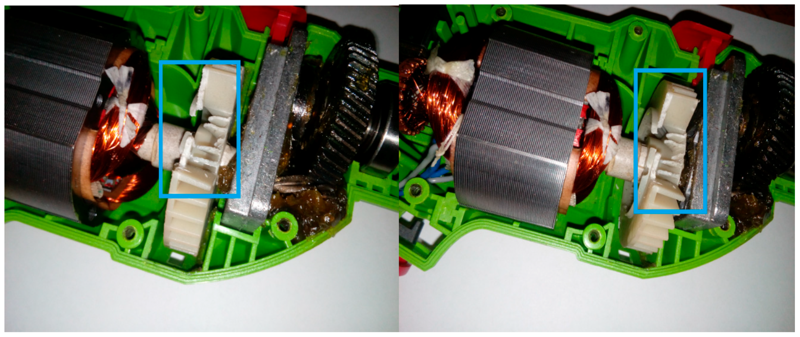
Figure 2.
Electric impact drill with a damaged gear train (indicated by the blue box).

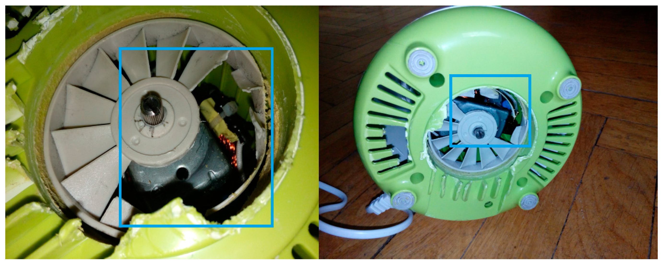
Figure 3.
Electric impact drill with a faulty fan (5 broken rotor blades; indicated by the blue box).
Figure 3.
Electric impact drill with a faulty fan (5 broken rotor blades; indicated by the blue box).

Figure 4.
Electric impact drill with a faulty fan (10 broken rotor blades; indicated by the blue box).
Figure 4.
Electric impact drill with a faulty fan (10 broken rotor blades; indicated by the blue box).

Figure 5.
Electric impact drill with a shifted brush (motor off; indicated by the blue box).

Figure 6.
Healthy blender.

Figure 7.
Blender with a faulty fan (2 broken rotor blades; indicated by the blue box).

Figure 8.
Blender with a faulty fan (5 broken rotor blades; indicated by the blue box).

Figure 9.
Flowchart of the proposed fault detection using smartphone and acoustic signals. NM: nearest mean; SVM: support vector machine.
Figure 9.
Flowchart of the proposed fault detection using smartphone and acoustic signals. NM: nearest mean; SVM: support vector machine.

Figure 10.
(a) Diagram of the experimental setup of the measurements using the smartphone. (b) Experimental setup of the blender and electric impact drill.
Figure 10.
(a) Diagram of the experimental setup of the measurements using the smartphone. (b) Experimental setup of the blender and electric impact drill.


Figure 11.
Flowchart of the proposed method of feature extraction, MSAF-RATIO-27-MULTIEXPANDED-4-GROUPS. FFT: Fast Fourier Transform; TCF: threshold of common frequency components.
Figure 11.
Flowchart of the proposed method of feature extraction, MSAF-RATIO-27-MULTIEXPANDED-4-GROUPS. FFT: Fast Fourier Transform; TCF: threshold of common frequency components.

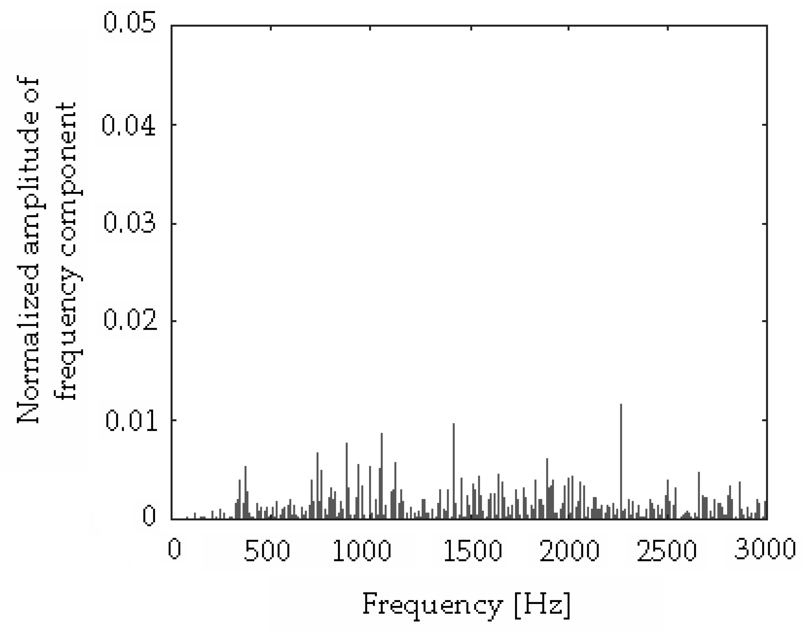
Figure 12.
Difference (|hd − ddgt|) using the MSAF-RATIO-27-MULTIEXPANDED-4-GROUPS method. hd refers to the healthy electric impact drill; ddgt refers to the electric impact drill with damaged gear train.
Figure 12.
Difference (|hd − ddgt|) using the MSAF-RATIO-27-MULTIEXPANDED-4-GROUPS method. hd refers to the healthy electric impact drill; ddgt refers to the electric impact drill with damaged gear train.

Figure 13.
Difference (|hd − dfive|) using the MSAF-RATIO-27-MULTIEXPANDED-4-GROUPS method. dfive refers to the electric impact drill with a faulty fan (5 broken rotor blades).
Figure 13.
Difference (|hd − dfive|) using the MSAF-RATIO-27-MULTIEXPANDED-4-GROUPS method. dfive refers to the electric impact drill with a faulty fan (5 broken rotor blades).

Figure 14.
Difference (|hd − dten|) using the MSAF-RATIO-27-MULTIEXPANDED-4-GROUPS method. dten refers to the electric impact drill with a faulty fan (10 broken rotor blades).
Figure 14.
Difference (|hd − dten|) using the MSAF-RATIO-27-MULTIEXPANDED-4-GROUPS method. dten refers to the electric impact drill with a faulty fan (10 broken rotor blades).

Figure 15.
Difference (|ddgt − dfive|) using the MSAF-RATIO-27-MULTIEXPANDED-4-GROUPS method.

Figure 16.
Difference (|ddgt − dten|) using the MSAF-RATIO-27-MULTIEXPANDED-4-GROUPS method.

Figure 17.
Difference (|dfive − dten|) using the MSAF-RATIO-27-MULTIEXPANDED-4-GROUPS method.

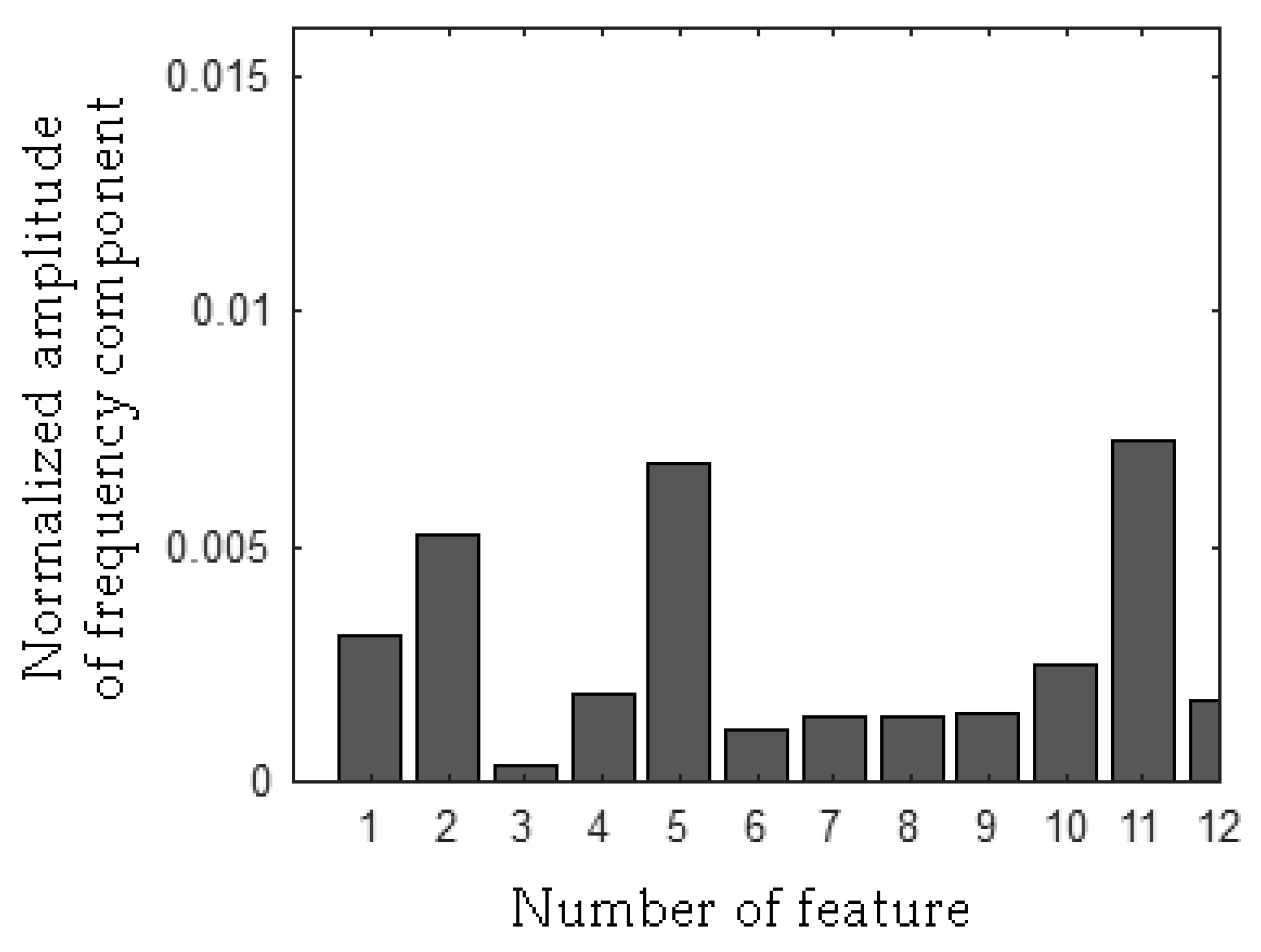
Figure 18.
Values of features of the vector hd (healthy electric impact drill).

Figure 19.
Values of features of the vector ddgt (electric impact drill with damaged gear train).

Figure 20.
Values of features of the vector dfive (electric impact drill with a faulty fan with 5 broken rotor blades).
Figure 20.
Values of features of the vector dfive (electric impact drill with a faulty fan with 5 broken rotor blades).

Figure 21.
Values of features of the vector dten (electric impact drill with a faulty fan with 10 broken rotor blades).
Figure 21.
Values of features of the vector dten (electric impact drill with a faulty fan with 10 broken rotor blades).

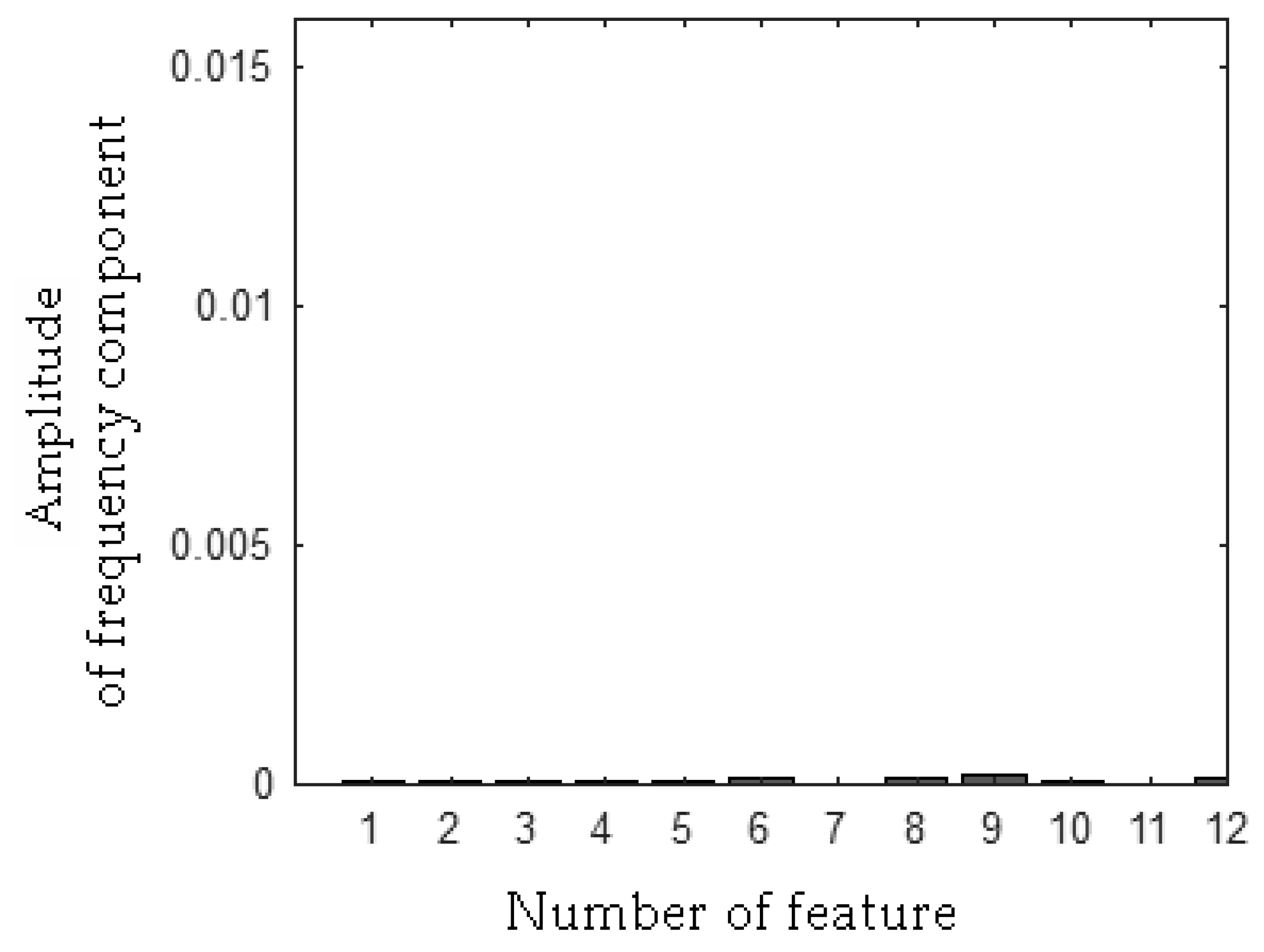
Figure 22.
Values of features (without amplitude normalization) of the electric impact drill with a shifted brush (motor off).
Figure 22.
Values of features (without amplitude normalization) of the electric impact drill with a shifted brush (motor off).

Figure 23.
Values of features of the healthy blender.

Figure 24.
Values of features of the blender with (2 broken rotor blades).

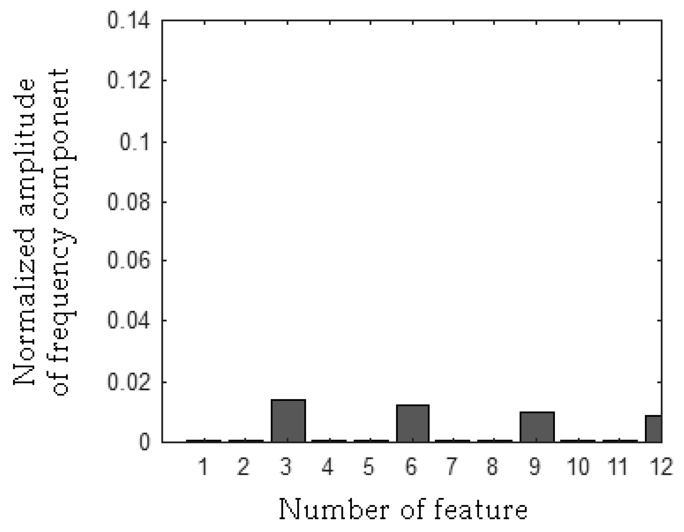
Figure 25.
Values of features of the blender with a faulty fan (5 broken rotor blades).

Figure 26.
SVM model (for the example two features of X and Y).


Table 1.
Values of features of the vector hd (healthy electric impact drill).
| Value of Feature | |||
|---|---|---|---|
| 0.002389 | 0.003904 | 0.000189 | 0.001208 |
| 0.006762 | 0.000414 | 0.000723 | 0.000510 |
| 0.002307 | 0.003273 | 0.006422 | 0.001074 |
Table 2.
Values of features of the vector ddgt (electric impact drill with damaged gear train).
| Value of Feature | |||
|---|---|---|---|
| 0.002216 | 0.002847 | 0.000434 | 0.001511 |
| 0.002599 | 0.000233 | 0.000449 | 0.000704 |
| 0.001381 | 0.001658 | 0.002525 | 0.003383 |
Table 3.
Values of features of the vector dfive (electric impact drill with a faulty fan with 5 broken rotor blades).
Table 3.
Values of features of the vector dfive (electric impact drill with a faulty fan with 5 broken rotor blades).
| Value of Feature | |||
|---|---|---|---|
| 0.001651 | 0.004912 | 0.012708 | 0.003004 |
| 0.006170 | 0.014284 | 0.002118 | 0.001150 |
| 0.005399 | 0.002338 | 0.004434 | 0.007732 |
Table 4.
Values of features of the vector dten (electric impact drill with a faulty fan with 10 broken rotor blades).
Table 4.
Values of features of the vector dten (electric impact drill with a faulty fan with 10 broken rotor blades).
| Value of Feature | |||
|---|---|---|---|
| 0.003078 | 0.005273 | 0.000338 | 0.001864 |
| 0.006732 | 0.001138 | 0.001405 | 0.001365 |
| 0.001450 | 0.002512 | 0.007226 | 0.001697 |
Table 5.
Values of features of the electric impact drill with a shifted brush (motor off).
| Value of Feature | |||
|---|---|---|---|
| 0.0001033 | 0.0000653 | 0.0000749 | 0.0001034 |
| 0.0000923 | 0.0001318 | 0.0000371 | 0.0001065 |
| 0.0002000 | 0.0000667 | 0.0000323 | 0.0001145 |
Table 6.
Values of features of the healthy blender.
| Value of Feature | |||
|---|---|---|---|
| 0.002236667 | 0.012738667 | 0.001946333 | 0.003069333 |
| 0.020384 | 0.001906667 | 0.002930667 | 0.013355 |
| 0.001388333 | 0.003803 | 0.014756 | 0.002679333 |
Table 7.
Values of features of the blender with a faulty fan (2 broken rotor blades).
| Value of Feature | |||
|---|---|---|---|
| 0.000446667 | 0.000665333 | 0.014109667 | 0.000445333 |
| 0.000905333 | 0.0125 | 0.000423667 | 0.000836333 |
| 0.009938 | 0.000623333 | 0.000480667 | 0.008561667 |
Table 8.
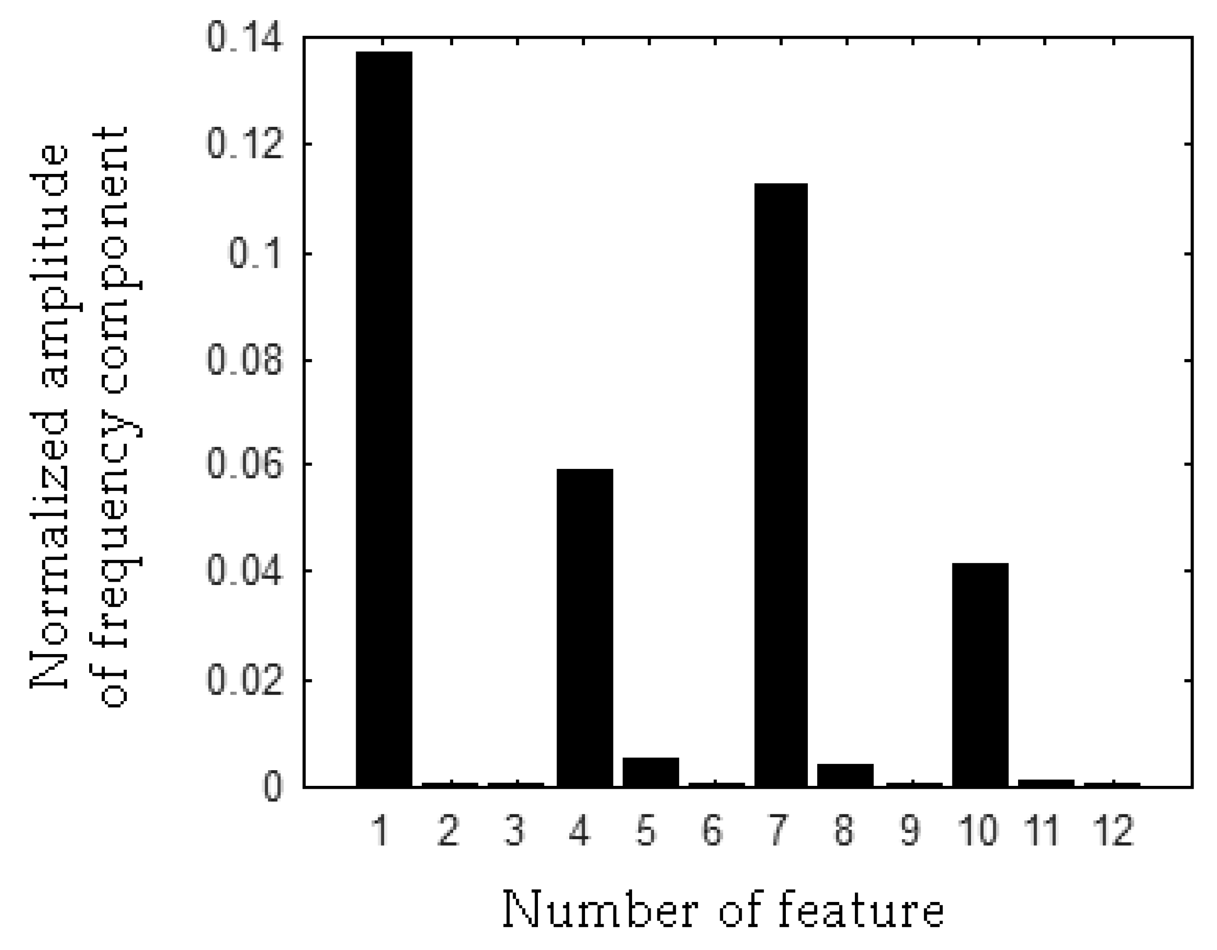
Values of features of the blender with a faulty fan (5 broken rotor blades).
| Value of Feature | |||
|---|---|---|---|
| 0.136920667 | 0.000855333 | 0.000701667 | 0.059152333 |
| 0.005108 | 0.000530667 | 0.112844667 | 0.004174333 |
| 0.000560667 | 0.041357333 | 0.001391333 | 0.000543 |
Table 9.
Analysis of the acoustic signals of the electric impact drill using the MSAF-RATIO-27-MULTIEXPANDED-4-GROUPS method (12 analysed frequency components) and the NM.
Table 9.
Analysis of the acoustic signals of the electric impact drill using the MSAF-RATIO-27-MULTIEXPANDED-4-GROUPS method (12 analysed frequency components) and the NM.
| Type of Acoustic Signal | EEID [%] |
|---|---|
| Healthy electric impact drill | 100 |
| Electric impact drill with a damaged gear train | 100 |
| Electric impact drill with a faulty fan (5 broken rotor blades) | 84 |
| Electric impact drill with a faulty fan (10 broken rotor blades) | 96 |
| Electric impact drill with a shifted brush (motor off) | 100 |
| TEEID [%] | |
| Total efficiency of recognition of the electric impact drill | 96 |
Table 10.
Analysis of the acoustic signals of the electric impact drill using the MSAF-RATIO-27-MULTIEXPANDED-4-GROUPS method (12 analysed frequency components) and SVM.
Table 10.
Analysis of the acoustic signals of the electric impact drill using the MSAF-RATIO-27-MULTIEXPANDED-4-GROUPS method (12 analysed frequency components) and SVM.
| Type of Acoustic Signal | EEID [%] |
|---|---|
| Healthy electric impact drill | 96 |
| Electric impact drill with a damaged gear train | 100 |
| Electric impact drill with a faulty fan (5 broken rotor blades) | 76 |
| Electric impact drill with a faulty fan (10 broken rotor blades) | 72 |
| Electric impact drill with a shifted brush (motor off) | 100 |
| TEEID [%] | |
| Total efficiency of recognition of the electric impact drill | 88.8 |
Table 11.
Analysis of the acoustic signals of the blender using the MSAF-RATIO-27-MULTIEXPANDED-4-GROUPS method (12 analysed frequency components) and the NM.
Table 11.
Analysis of the acoustic signals of the blender using the MSAF-RATIO-27-MULTIEXPANDED-4-GROUPS method (12 analysed frequency components) and the NM.
| Type of Acoustic Signal | EEID [%] |
|---|---|
| Healthy blender | 100 |
| Blender with a faulty fan (2 broken rotor blades) | 100 |
| Blender with a faulty fan (5 broken rotor blades) | 100 |
| TEB [%] | |
| Total efficiency of recognition of the blender | 100 |
Table 12.
Analysis of the acoustic signals of the blender using the MSAF-RATIO-27-MULTIEXPANDED-4-GROUPS method (12 analysed frequency components) and SVM.
Table 12.
Analysis of the acoustic signals of the blender using the MSAF-RATIO-27-MULTIEXPANDED-4-GROUPS method (12 analysed frequency components) and SVM.
| Type of Acoustic Signal | EEID [%] |
|---|---|
| Healthy blender | 82 |
| Blender with a faulty fan (2 broken rotor blades) | 100 |
| Blender with a faulty fan (5 broken rotor blades) | 100 |
| TEB [%] | |
| Total efficiency of recognition of the blender | 94.11 |
© 2018 by the author. Licensee MDPI, Basel, Switzerland. This article is an open access article distributed under the terms and conditions of the Creative Commons Attribution (CC BY) license (http://creativecommons.org/licenses/by/4.0/).
Share and Cite
MDPI and ACS Style
Glowacz, A. Recognition of Acoustic Signals of Commutator Motors. Appl. Sci. 2018, 8, 2630. https://0-doi-org.brum.beds.ac.uk/10.3390/app8122630
AMA Style
Glowacz A. Recognition of Acoustic Signals of Commutator Motors. Applied Sciences. 2018; 8(12):2630. https://0-doi-org.brum.beds.ac.uk/10.3390/app8122630
Chicago/Turabian StyleGlowacz, Adam. 2018. "Recognition of Acoustic Signals of Commutator Motors" Applied Sciences 8, no. 12: 2630. https://0-doi-org.brum.beds.ac.uk/10.3390/app8122630
Note that from the first issue of 2016, this journal uses article numbers instead of page numbers. See further details here.