Distributed Kernel Extreme Learning Machines for Aircraft Engine Failure Diagnostics

Abstract

Kernel extreme learning machine (KELM) has been widely studied in the field of aircraft engine fault diagnostics due to its easy implementation. However, because its computational complexity is proportional to the training sample size, its application in time-sensitive scenarios is limited. Therefore, in the case of largescale samples, the original KELM is difficult to meet the real-time requirements of aircraft engine onboard condition. To address this shortcoming, a novel distributed kernel extreme learning machines (DKELMs) algorithm is proposed in this paper. The distributed subnetwork is adopted to reduce the computational complexity, and then the likelihood probability and Dempster-Shafer (DS) evidence theory is used to design the fusion scheme to ensure the accuracy after fusion is not reduced. Afterwards, the verification on the benchmark datasets shows that the algorithm can greatly reduce the computational complexity and improve the real-time performance of the original KELM algorithm without sacrificing the accuracy of the model. Finally, the performance estimation and fault pattern recognition experiments of an aircraft engine show that, compared with the original KELM algorithm and support vector machine (SVM) algorithm, the proposed algorithm has the best performance considering both real-time capability and model accuracy.

1. Introduction

Aircraft engine is a mission-critical mechanical system [1] with complicated structure and poor operating conditions [2], and its stable and reliable operation is of great importance to the flight safety [3]. During its whole service life, the performance of the aircraft engine degrades gradually due to fouling [4] and corrosion [5] of blades, and the increase of tip clearance [6]. In addition, foreign or inner object damage [7] may cause sharp felling of performance. In reverse, decline of the performance would result in thrust loss of the aircraft engine, and then the fuel is required to guarantee the required thrust of the aircraft engine [8]. Thus the operating point would be closer to the surge margin and the exhaust gas temperature (EGT) would increase. Consequently, the reliability would be jeopardized by the former case and the service life would be jeopardized by the latter case. For the purpose of improving the reliability and reducing the maintenance cost, the condition-based maintenance (CBM) system is adopted to facilitate the mission scheduling [9]. Fault diagnostics and prognostics constitute two typical portions of the CBM system. Diagnostics is to detect the fault and then carry out the identification and isolation [10], and the main purpose of prognostics is to predict the aircraft engine performance after the degradation and failure [11]. Quantifiable evaluation of aircraft engine degradation is the core to the CBM system. In terms of the economic endurance, effective health assessment and reliable performance prediction are conducive to effectively cut down flight costs and improve the reliability and availability [12]. In addition, by utilizing the performance prediction technology reasonably, the aircraft engine can be restored to healthy state before failures, and thus catastrophic accidents can be avoided.

The existing diagnostic methods for aircraft engine mainly include the model-based method [13,14] and the data-driven method [15,16]. For the model-based approach, mathematical models are usually required to assess the internal characteristics of the aircraft engine failure. However, the failure mechanism of the aircraft engine is usually extremely complex, and it is hard to establish a volumetric dynamic or thermodynamics model that can predict the health state and is applicable to the whole working condition range [17] with high reliability. In the last few years, with the fast evolution of machine learning methods and the continuous accumulation of flight cycle data, the data-driven methods have attracted more and more attention in the field of diagnostics for aircraft engine [18]. In addition, some successful developments of aircraft engine CBM system are based on data-driven methods, and a great deal of practical cases have verified that the data-driven method can improve the accuracy of engine fault diagnosis and performance prediction without additional need for internal understanding of aircraft engine [19,20].

Common data-driven methods mainly include artificial neural networks (ANNs) [21,22], support vector machine (SVM) [23] and statistical feature analysis [24], etc. The nonlinear mapping capabilities of neural networks are excellent, and thus the application in fault diagnosis and performance prediction for aircraft engine is developed rapidly. The general structure of neural network usually involves input layer, hidden layer and output layer [25]. The training method based on gradient is widely used in the iterative adjustment of network structure parameters, thus in the practical application, the slow learning speed is a common problem of neural networks [26]. In order to improve the training speed, extreme learning machine (ELM) is proposed to train the single hidden layer feed-forward neural networks (SLFNs), which is one of the most popular networks. Different from the traditional ANNs, ELM randomly assigns the network parameter, and then the output weight is determined analytically [27]. Compared with the traditional network, ELM has much faster training and testing speed and better or similar generalization performance [28,29]. Due to the random configuration of parameters, ELM has advantages of high computational efficiency and easy implementation, but at the same time, the random characteristics also lead to fluctuating and unstable network performance [30]. Huang et al. proposed the KELM method by introducing kernel functions into ELM [31]. Similar to the SVM method, the training sample error and weight minimization are considered comprehensively in KELM, where the tradeoffs are represented by regular parameter.

Extensive experiments have shown that KELM has better generalization ability than ELM in most cases, and tends to perform better for dealing with classification as well as regression problems [32,33]. However, the original KELM has two obvious limitations. Firstly, due to the inverse calculation of an $n\times n$ matrix, the overall computational complexity increases cubically with n. Thus the training process would be computationally impossible when the number of training samples is too large even if the problem is linearly solvable. In addition, the network constructed by KELM contains all the training samples, and such a network would be too complex due to lack of sparsity, which is likely to lead to overfitting problem. Due to the limiting onboard computing power of aircraft engine, the data driven methods on board are required to have high computational efficiency and good real-time performance [34]. Aiming at the above lack of original KELM, we proposed a novel DKLEMs algorithm, where the network structure of the original KELM is replaced by some distributed sub-networks, and then the fusion of information form each sub-network is conducted subsequently. The new network structure includes feature input layer, distributed machines layer, fusion layer and output layer. In order to verify the validity of distributed kernel extreme learning machines (DKELMs) algorithm, performance comparison among the proposed algorithm, the original KELM algorithm and SVM algorithm are carried out in both regression and classification benchmark dataset. Finally, for practical verification of the proposed algorithm, experiments are carried out on performance degeneration estimation and failure patterns identification for an aircraft engine.

The remainder of this paper is organized as follows: In Section 2 we will briefly review the original KELM algorithm and further propose the distributed KELM framework. The fusion approach of distributed machines for both classification and regression problems are presented and the derivation is given in detail in Section 3. In Section 4, performance evaluation on regression and classification benchmark datasets are conducted, where DKELMs are compared with original KELM and SVM algorithms. In Section 5, the proposed DKELMs algorithm is applied into failure diagnostics of aircraft engine. Conclusions are given in Section 6.

2. Review of Basic and Kernel Elm

In order to improve the training speed of SLFNs network, Huang proposed the ELM algorithm. By randomly assigning network parameters and determining output weights analytically, ELM can greatly improve the learning speed. Later, Huang et. al introduced kernel method into the basic ELM and proposed the KELM algorithm, which can be directly applied into regression and multi-class classification problems. This section provides a brief review of the basic ELM and KELM algorithms.

2.1. Elm

For the structural form of SLFNs, Huang et al. proposed ELM to improve the network training speed, and then extended the hypothesis of ELM from neuron hidden nodes to other hidden nodes. Training samples can be represented as ${\left\{{\mathit{x}}_i,t_i\right\}}_{i=1}^n$, where n is the training samples number, ${\mathit{x}}_i$ denotes input of $ith$ sample with m-dimension and $t_i$ is output of $ith$ sample. Then, given the input vector $\mathit{x}$, the output of SLFNs with L hidden nodes can be written as

$$\begin{array}{c}\hfill f(\mathit{x})={\displaystyle \sum _{i=1}^L}{\beta }_i{h}_i(\mathit{x})={\mathit{h}}^T(\mathit{x})\mathit{\beta }\end{array}$$

(1)

where $\mathit{h}(\mathit{x})={\left[h_1(\mathit{x})\cdots h_L(\mathit{x})\right]}^T$ denotes the hidden output, and $\mathit{\beta }={\left[{\beta }_1\cdots {\beta }_L\right]}^T$ denotes the output weights. Assume that outputs of these n training samples can be approximated with zero errors, the compact formulation is as follows

$$\begin{array}{c}\hfill H\mathit{\beta }=\mathit{t}\end{array}$$

(2)

where $H={\left[\mathit{h}({\mathit{x}}_1)\cdots \mathit{h}({\mathit{x}}_n)\right]}^T$ is named as hidden output matrix. The solution of output weights $\mathit{\beta }$ only involves a simple linear equation, and the solution may be equivalent to the minimization of training error i.e., $min∥H\mathit{\beta }-\mathit{t}∥$. The optimal estimation of output weights may be represented by the Moore-Penrose generalized inverse [35] $H^{†}$ as follows

$$\begin{array}{c}\hfill \widehat{\mathit{\beta }}=H^{†}\mathit{t}\end{array}$$

(3)

Generally, the orthogonal projection can be used to solve the generalized inverse $H^{†}$. If $H^{T}H$ is nonsingular, $H^{†}={(H^{T}H)}^{-1}{H}^T$, or if $H{H}^T$ is nonsingular, $H^{†}=H^T{(H{H}^T)}^{-1}$.

2.2. Kernel ELM

Kernel ELM was developed from ELM using the kernel transforming technology, which enables it to have better generalization performance than ELM due to the kernel transformation from input space to kernel space. Minimizing the training errors as well as the output weights at the same time, KELM can be derived as the following constrained optimization form

$$\begin{array}{c}\hfill \begin{array}{c}\underset{\mathit{\beta }}{min}\frac{1}{2}{\parallel \mathit{\beta }\parallel }_2^2+\frac{C}{2}{\displaystyle \sum _{i=1}^n}{\epsilon }_i^2\hfill \\ s.t.{\mathit{\phi }}^T({\mathit{x}}_i)\mathit{\beta }=t_i-{\epsilon }_i,i=1,2,\cdots ,n\hfill \end{array}\end{array}$$

(4)

where $\mathit{\phi }(·)$ defines the kernel transformation from input space to kernel space, ${\epsilon }_i$ is the $ith$ training error, the specified parameter C is used to represent the tradeoff between $\mathit{\beta }$ and $\mathit{\epsilon }$.

Through proper kernel transformation, the linear unsolvable problem in the input space can be converted to a linear solvable problem in the kernel space. According to the Karush-Kuhn-Tucker (KKT) theorem and after introducing the Lagrange multiplier ${\alpha }_i$, the following dual optimization problem can be utilized to solve the output weights $\mathit{\beta }$

$$\begin{array}{c}\hfill \underset{\mathit{\beta },\mathit{\alpha },\mathit{\epsilon }}{min}\left\{L=\frac{1}{2}{\parallel \mathit{\beta }\parallel }_2^2+\frac{C}{2}{\displaystyle \sum _{i=1}^n}{\epsilon }_i^2-{\displaystyle \sum _{i=1}^n}{\alpha }_i\left({\mathit{\phi }}^T({\mathit{x}}_i)\mathit{\beta }-t_i+{\epsilon }_i\right)\right\}\end{array}$$

(5)

Take the partial derivatives and make them zero, the KKT conditions can be written as

$$\begin{array}{c}\hfill \begin{array}{c}\frac{\partial L}{\partial {\beta }_j}=0,j=1,\cdots ,L\to \mathit{\beta }={\Phi }^T\mathit{\alpha }\hfill \\ \frac{\partial L}{\partial {\epsilon }_i}=0,i=1,\cdots ,n\to \mathit{\alpha }=C\mathit{\epsilon }\hfill \\ \frac{\partial L}{\partial {\alpha }_i}=0,i=1,\cdots ,n\to \Phi \mathit{\beta }-\mathit{t}+\mathit{\epsilon }=\mathit{0}\hfill \end{array}\end{array}$$

(6)

where $\Phi ={\left[\mathit{\phi }({\mathit{x}}_1)\cdots \mathit{\phi }({\mathit{x}}_n)\right]}^T$ denotes the kernel output function. With a little bit of simple substitution and derivation, the output function may be transformed into the following expression

$$\begin{array}{c}\hfill f(\mathit{x})={\mathit{\phi }}^T(\mathit{x}){\Phi }^T\mathit{\alpha }={\mathit{\phi }}^T(\mathit{x}){\Phi }^T{\left(I_n/C+\Phi {\Phi }^T\right)}^{-1}\mathit{t}\end{array}$$

(7)

where $I_n$ denotes identity matrix with n-dimension, and based on the ridge regression theory, the enhancement of the regulation item $I_n/C$ is able to improve the generalization performance [35]. For the convenience of calculation, kernel transformation is uniformly written as inner product, and the kernel matrix is defined as

$$\begin{array}{c}\hfill K=\Phi {\Phi }^T:K_{i,j}=\mathit{\phi }({\mathit{x}}_i)·\mathit{\phi }({\mathit{x}}_j)=k({\mathit{x}}_i,{\mathit{x}}_j)\end{array}$$

(8)

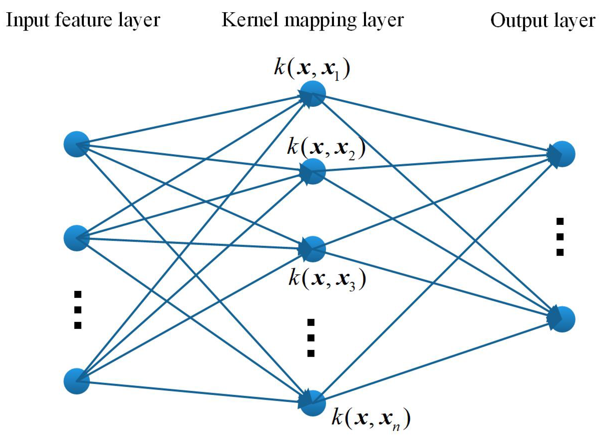
The network structure of the original KELM algorithm is illustrated by Figure 1, including the input feature layer, the kernel mapping layer and the output layer. In the kernel mapping layer, all the training samples are used as the hidden nodes. Thus, the output function could be represented in the compact formulation as

$$\begin{array}{c}\hfill f(\mathit{x})=\left[k(\mathit{x},{\mathit{x}}_1)\cdots k(\mathit{x},{\mathit{x}}_n)\right]\mathit{\alpha }\end{array}$$

(9)

where $\mathit{\alpha }={\left(I_n/C+K\right)}^{-1}\mathit{t}$ denotes the output weights in terms of kernel mapping.

KELM is similar to the SVM in that it only needs to define the kernel matrix without needing knowledge about the specific kernel mapping and the dimension of kernel space. It can be proved theoretically that if the expression of SVM does not contain bias terms, the result of KELM is consistent with that of least squares SVM. KELM adopts structural risk minimization strategy to ensure good generalization performance by comprehensively considering empirical risks as well as confidence intervals. Solution of the weight $\mathit{\alpha }$ mainly involves the inverse calculation of an $n\times n$ matrix. If there are too many training samples in the data set, the network structure redundancy may jeopardize the computational efficiency and generalization performance, and even lead to the failure of inverse operation.

3. Distributed Kernel Extreme Learning Machines

It has been proved theoretically that the original KELM algorithm has the approaching ability for any continuous functions and classifying ability for any disjoint regions. However, the KELM network is constructed by using all the training samples, and inevitably, the network structure that lacks sparsity may be very redundant. When large datasets are involved, the redundancy of the network would lead to the decrease of computing efficiency, overfitting problem and lower generalization performance. In addition, the issue of excessive storage expense and memory exhaustion problem must be considered as well. To this end, a novel DKELMs algorithm is proposed in this section, where the network structure of the original KELM is replaced by multiple subnetworks to improve its performance for largescale datasets.

3.1. Distributed Framework

The framework of the proposed DKELMs algorithm is illustrated by Figure 2, including feature samples input and output, distributed subnetworks, fusion module and estimated output. In the distributed subnetworks, l learning machines are used to process the input features, and the fusion module can mix the outputs of l subnetworks. The entire training dataset can be represented as ${\left\{{\mathit{x}}_i,t_i\right\}}_i^n$, and divide it into l subsets. The training samples number of the $p_{th}$ subset is represented as $n_p$, and we have ${\displaystyle \sum _{p=1}^l}{n}_p=n$. The $p_{th}$ subset of training samples ${\left\{{\tilde{\mathit{x}}}_i,{\tilde{t}}_i\right\}}_1^{n_p}$ is used to construct the $p_{th}$ subnetwork DKELM p in Figure 2. For the $p_{th}$ subnetwork, the hidden nodes number is $n_p$, and the portion kernel matrix ${\tilde{K}}_p$ is defined as follows

$$\begin{array}{c}\hfill {\tilde{K}}_p:{\tilde{K}}_{i,j}=k({\tilde{\mathit{x}}}_i,{\mathit{x}}_j),i=1,\cdots ,n_p,j=1,\cdots ,n\end{array}$$

(10)

For the inversion calculation of the non-square matrix ${\tilde{K}}_p$, the generalized inverse theory should be used, and taking no account of regular terms, the kernel output weights can be represented as ${\tilde{\mathit{\alpha }}}_p={\tilde{K}}_p^{†}\mathit{t}={({\tilde{K}}_p{\tilde{K}}_p^T)}^{-1}{\tilde{K}}_p\mathit{t}$. According to the ridge regression theory, adding a small positive deviation to the diagonal value of ${\tilde{K}}_p{\tilde{K}}_p^T$ can improve the stability of the solution. Then, the model output of subnetwork DKELM p can be expressed as follows

$$\begin{array}{c}\hfill {\tilde{\mathit{\alpha }}}_p={(I/C+{\tilde{K}}_p{\tilde{K}}_p^T)}^{-1}{\tilde{K}}_p\mathit{t}\end{array}$$

(11)

$$\begin{array}{c}\hfill f_p(\mathit{x})=\left[k(\mathit{x},{\tilde{\mathit{x}}}_1)\cdots k(\mathit{x},{\tilde{\mathit{x}}}_{n_p})\right]{\tilde{\mathit{\alpha }}}_p\end{array}$$

(12)

The proposed DKELMs algorithm can replace the inversion of a $n\times n$ matrix by inversions of $n_p\times n_p$ matrix in l times. When it comes to largescale dataset, the computation complexity can be largely cut down. Given the kernel function and a training dataset ${\left\{{\mathit{x}}_i,t_i\right\}}_i^n$, the $p_{th}$ subnetwork DKELM p can be constructed as follows

• Divide ${\left\{{\mathit{x}}_i,t_i\right\}}_i^n$ into l subsets, and pick the $p_{th}$ subset ${\left\{{\tilde{\mathit{x}}}_i,{\tilde{t}}_i\right\}}_1^{n_p}$.
• Calculate the rectangular kernel matrix ${\tilde{K}}_p\in R^{n_p}\times R^n$.
• Calculate the kernel output weights ${\tilde{\mathit{\alpha }}}_p$ as Formula (11).
• Figure out the output of the subnetwork DKELM p for new input vector $\mathit{x}$ according to Formula (12).

In the fusion layer, output information of l parallel subnetworks should be taken into account comprehensively and come up with more excellent results. Therefore, a likelihood probability distribution-based regression fusion method is constructed for the regression problem, and for the classification problem, a classification fusion method based on DS evidence theory is designed.

3.2. Likelihood Probability Fusion

In the regression problem, for the input characteristics $\mathit{x}$, the output of l subnetworks can be represented as ${\left\{{\mu }_i,{\sigma }_i\right\}}_i^l$, where ${\mu }_i$ is the regression value of $i_{th}$ subnetwork and ${\sigma }_i$ is the standard deviation of the training process. Assuming that the predicted value of regression obeys gaussian distribution, the probability density function of each sub-learning machine regression value can be expressed as

$$\begin{array}{c}\hfill p_i\left(t|\mathit{x}\right)=\frac{1}{\sqrt{2\pi }{\sigma }_i}exp\left(-\frac{{\left(t-{\mu }_i\right)}^2}{2{\sigma }_i^2}\right)\end{array}$$

(13)

Thus, the probability density function of the comprehensive output of the learning unit is proportional to the product of the densification density output of the sub-learning machine

$$\begin{array}{c}\hfill p\left(t|\mathit{x}\right)\propto p_1\left(t|\mathit{x}\right)p_2\left(t|\mathit{x}\right)\cdots p_l\left(t|\mathit{x}\right)\end{array}$$

(14)

If we take the natural logarithm of the above expression and convert the product into a sum, the following relation can be obtained

$$\begin{array}{c}\hfill ln(p)\propto ln(p_1)+ln(p_2)+\cdots +ln(p_l)\end{array}$$

(15)

By substituting the probability density of the sub-learning machine, the comprehensive output probability density can be transformed into the form of quadratic function

$$\begin{array}{c}\hfill ln\left(p\left(t|\mathit{x}\right)\right)\propto -{\displaystyle \sum _1^l}\frac{{\left(t-{\mu }_i\right)}^2}{2{\sigma }_i^2}\end{array}$$

(16)

According to the principle of maximum likelihood probability, the maximum value of probability density is taken as the predicted value of regression

$$\begin{array}{c}\hfill \widehat{t}=\underset{y\in R}{argmin}{\displaystyle \sum _1^l}\frac{{\left(t-{\mu }_i\right)}^2}{2{\sigma }_i^2}\end{array}$$

(17)

3.3. DS Evidence Theory Fusion

A.P. Dempster used upper and lower limit probability to solve the multi-value mapping problem, marking the formal birth of DS evidence theory, and G. Shafer further developed the evidence theory, introduced the concept of trust function, and formed a set of mathematical methods of “evidence” and “combination” to deal with uncertain reasoning [36]. DS theory is a generalization of Bayesian inference method, which is mainly carried out by using Bayesian conditional probability in probability theory. It can represent “uncertainty” well and is widely used to deal with uncertain data.

In this subsection, DS evidence theory is introduced to design the classification fusion device of DKELMs algorithm. It is assumed that number of categories is k, and the $i_{th}$ category is represented as $c_i$. The identification framework is $U={\left\{c_i\right\}}_1^k$, and the mass function $m:2^U\to [0,1]$ satisfies two equations: $m(\varnothing )=0$ and ${\sum }_{C\subset U}m(C)=1$. The mass function $m(C)$ is the basic probability assignment of C, and denotes the degree of confidence.

For the classification problem, the output of each subnetwork can be transferred into the mass function by the softmax function, and the mass function outputs of l subnetworks can be expressed as $m_1,m_2,\cdots ,m_l$ respectively. For each proper subset C of U, the Dempster combination rules are

$$\begin{array}{c}\hfill m_1\oplus m_2\oplus \cdots \oplus m_l(C)=\frac{1}{\Omega }\sum _{C_1\bigcap C_2\bigcap \cdots \bigcap C_l=C}{m}_1(C_1)m_2(C_2)\cdots m_l(C_l)\end{array}$$

(18)

$$\begin{array}{c}\hfill \begin{array}{cc}\hfill \Omega & =\sum _{C_1\bigcap C_2\bigcap \cdots \bigcap C_l\ne \varnothing }{m}_1(C_1)m_2(C_2)\cdots m_l(C_l)\hfill \\ & =1-\sum _{C_1\bigcap C_2\bigcap \cdots \bigcap C_l=\varnothing }{m}_1(C_1)m_2(C_2)\cdots m_l(C_l)\hfill \end{array}\end{array}$$

(19)

where $\Omega$ is the normalization factor, and $1-\Omega$ reflects the degree of conflicts from different subnetworks. Let the proper subset C be a category $\left\{c_i\right\}$, and then the probability that a sample having input feature $\mathit{x}$ belongs to this category should be

$$\begin{array}{c}\hfill P(\mathit{x}\in c_i)=m_1\oplus m_2\oplus \cdots \oplus m_l(C)\end{array}$$

(20)

By synthesizing the output results of multiple subnetworks, the output after fusion is more accurate than that of the subnetworks, and not lower than the accuracy of the original KELM network. In addition, as the scale of each subnetwork is effectively controlled, the sparsity is improved and the overfitting problem is weakened to some extent. Furthermore, the decrease of computation results in higher learning speed.

4. Verification on Benchmark Datasets

For purposing verifying the validity and superiority of DKELMs algorithm, seven regression datasets and six classification datasets are selected [37], and DKELMs algorithm is compared with original KELM and SVM (n-SVR algorithm for regression and C-SVC algorithm for classification [38]). The input data of all datasets is normalized to $[-1,1]$, the output data of the regression dataset is normalized to $[0,1]$, and the output data of the classification dataset is represented by one-hot encoding. The hardware used for all simulations is a desktop computer, equipped with i5-7200U processor and 4GB running memory, and the software environment is MATLAB 7.11. Gaussian kernel function is selected, and the regular parameters and kernel parameters of KELM are selected by the fast leave-one-out (FLOO) method [39], while the adjustment parameters of DKELMs and SVM are selected by the experimental method.

4.1. Regression

The selected seven regression datasets are shown in

Table 1. Parameters of the regression dataset.

Datasets	#Attributes	#Train	#Test
Abalone	7	3133	1044
Airfoil sound	5	1127	376
Auto mpg	7	297	99
Bike sharing	11	549	183
Boston housing	13	380	126
Cpusmall	12	6144	2048
White wine quality	11	3674	1224

, and for each dataset, attributes number (#Attributes), training samples number (#Training) and testing samples number (#Testing) are given respectively. For regression problems, the following rooted mean square error ($RMSE$) is defined to describe the performance,

$$\begin{array}{c}\hfill RMSE=\sqrt{\frac{{\displaystyle \sum _{i=1}^N}{(t_i-{\widehat{t}}_i)}^2}{N}}\end{array}$$

(21)

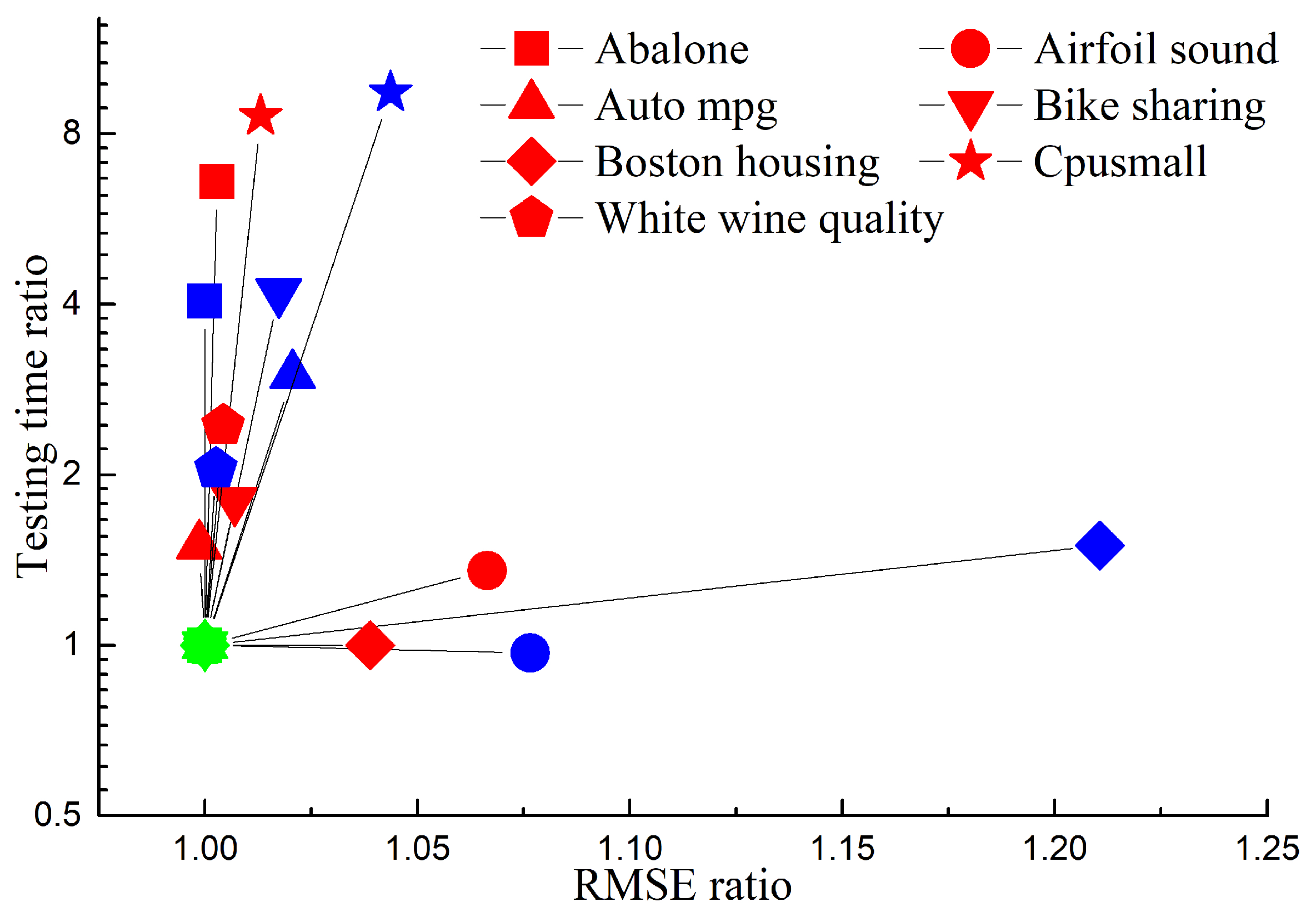
where $t_i$ denotes the output of testing sample, ${\widehat{t}}_i$ is the corresponding estimation, and N is the testing samples number. As a classic regression algorithm, n-support vector regression (n-SVR) algorithm would be utilized in this subsection for comparison experiments in the benchmark regression problem dataset with original KELM and proposed DKELMs algorithms. The regression performance comparison among the three algorithms is shown in

Table 2. Performance of distributed KELM on regression benchmark datasets.

Datasets	Algorithm	RMSE	Training Time/s	Testing Time/s
Abalone	KELM	0.0708	0.3725	0.0546
	DKELMs	0.0706	0.0310	0.0083
	n-SVR	0.0706	17.4184	0.0336
Airfoil sound	KELM	0.0738	0.0364	0.0088
	DKELMs	0.0692	0.0295	0.0065
	n-SVR	0.0745	1.1691	0.0063
Auto mpg	KELM	0.0727	0.0020	0.0003
	DKELMs	0.0728	0.0013	0.0002
	n-SVR	0.0743	0.0093	0.0006
Bike sharing	KELM	0.0290	0.0066	0.0009
	DKELMs	0.0288	0.0028	0.0005
	n-SVR	0.0293	0.0409	0.0021
Boston housing	KELM	0.0641	0.0040	0.0010
	DKELMs	0.0617	0.0037	0.0010
	n-SVR	0.0747	0.0630	0.0015
Cpusmall	KELM	0.0232	1.4076	0.1563
	DKELMs	0.0229	0.0094	0.0182
	n-SVR	0.0239	12.3305	0.1721
White wine quality	KELM	0.1180	0.2140	0.0838
	DKELMs	0.1175	0.0658	0.0343
	n-SVR	0.1178	0.3859	0.0703

, in which $RMSE$, training time and testing time of each algorithm are listed respectively. As can be seen from Table 2, DKELMs has lower training time and testing time than KELM, and is of similar or higher accuracy. After adopting distributed structure, DKLEMs does not reduce the accuracy of regression prediction. Moreover, the fact that each subnetwork is composed of a smaller training subset enables DKELMs to have a higher sparsity than KELM and maintain a similar or better regression accuracy. Since DKELMs takes the calculation of multiple smaller networks, replacing the calculation of large networks containing all samples, and replacing the matrix inverse calculation of $n\times n$ matrix with the calculation of multiple small matrix inverses, the training time is greatly shortened, and the test time is also shortened on the whole. The reduction in computation is particularly evident in datasets with large sample sizes. The regression accuracy and testing time of n-SVR algorithm are close to KELM, but due to too many support vector points when dealing with regression problems, the training process is very time-consuming in most cases. In the application of failure diagnostics for aircraft engine, offline training and online testing are often adopted, so the testing time can better reflect the real-time performance than the training time. Therefore, in Figure 3, the proposed algorithm is compared with the original KELM and n-SVR algorithms in detail from the perspectives of $RMSE$ and testing time. The horizontal and vertical coordinates in the figure both represent the ratio, and the denominator is the corresponding value of DKELMs algorithm, so all the green points are at the (1,1) coordinate. As can be seen from the figure, the (1,1) coordinate is almost in the bottom left corner, which means that in all seven regression datasets, for both KELM and n-SVR algorithms, their $RMSE$s and testing time are higher than or similar to DKELMs algorithm. Considering the precision, training time and test time comprehensively, the proposed DKELMs algorithm is obviously superior to KELM algorithm and n-SVR algorithm in terms of regression problems.

4.2. Classification

Besides the regression case, the proposed DKELMs algorithm is also verified for classifying application. The selected six classification datasets are listed in

Table 3. Parameters of the classification dataset.

Datasets	Attributes	Classes	#Train	#Test
Wine	13	3	134	45
Handwritten digits	16	10	8255	2751
Iris	4	3	113	38
Page paper	10	5	4105	1368
Segment	19	7	1733	577
Vehicle	18	4	635	211

, where classes number (#Classes) and parameters described before are given respectively for each dataset. C-support vector classification (C-SVC) algorithm is usually used to deal with classification problems, and it would be treated as a contrast method in this subsection. In order to measure the classification ability of the algorithm, the correct rate is defined as: the number of correctly classified testing samples divided by the number of all testing samples. The performance comparison among original KELM, proposed DKELMs and C-SVC algorithms is given in

Table 4. Performance of distributed KELM on classification benchmark datasets.

Datasets	Algorithm	Correct Rate	Training Time/s	Testing Time/s
Wine	KELM	95.56%	0.0006	0.0002
	DKELMs	97.78%	0.0002	0.0001
	C-SVC	93.33%	0.0007	0.0002
Handwritten digits	KELM	98.15%	3.7564	0.3898
	DKELMs	98.51%	0.6444	0.2424
	C-SVC	97.42%	0.3605	0.2121
Iris	KELM	94.74%	0.0008	0.0001
	DKELMs	97.37%	0.0004	0.0001
	C-SVC	92.11%	0.0005	0.0001
Page	KELM	95.76%	0.6667	0.0931
	DKELMs	96.49%	0.3854	0.0500
	C-SVC	95.91%	0.1211	0.0212
Segment	KELM	96.71%	0.1071	0.0210
	DKELMs	97.05%	0.0644	0.0184
	C-SVC	96.88%	0.0419	0.0067
Vehicle	KELM	84.36%	0.0109	0.0023
	DKELMs	84.83%	0.0090	0.0010
	C-SVC	83.89%	0.0553	0.0027

, where correct rate, training time and testing time of each algorithm are listed respectively.

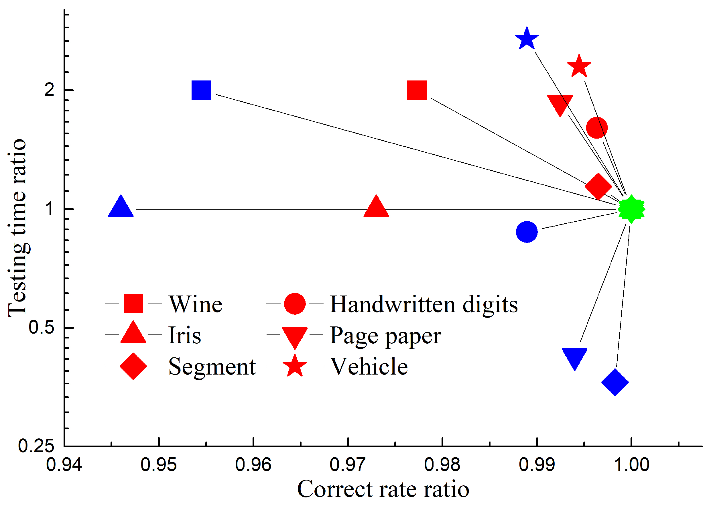
As shown in Table 4, in terms of correct rate, C-SVC and KELM algorithms are comparable, but proposed DKELMs algorithm generally tends to have higher or similar $RMSE$ than them. In addition, compared with original KELM algorithm, DKELMs can significantly reduce the training time and testing time. Each distributed subnetwork processes the input vector according to its own kernel nodes and generates independent classified probability. Then the DS evidence theory based fusion method can effectively synthesize the classified probability of subnetworks and improve the correct rate, so that the classification results of DKELMs algorithm have similar or even higher confidence than the original KELM algorithm. In addition, compared with the KELM algorithm, due to the advantages of sparse distributed structure, in terms of computational efficiency, the proposed algorithm can greatly cut down the training time for datasets with large sample size, and also cut down the testing time as a whole. In Figure 4, DKELMs algorithm is compared with the original KELM and C-SVC algorithms in detail from the perspectives of correct rate and testing time. Similar to the reason in Figure 3, all the green points corresponding to DKELMs algorithm are at the (1,1) coordinate. As can be seen from the figure, the (1,1) coordinate is at the far right, which means that for all six classification datasets, the correct rate of DKELMs is higher than two other algorithms. In addition, the ordinates of five red points are greater than 1, meaning that compared with the KELM algorithm, DKELMs algorithm can cut down the testing time in these five datasets. Compared with the KELM algorithm, DKELMs failed to reduce the testing time in the iris data set. This is because the iris dataset is too small, so the testing time of each algorithm is very small and there is no room for improvement. There are three blue points whose ordinates are less than 1, meaning that the testing time of C-SVC is less than DKELMs algorithm in handwritten digits dataset, page paper dataset and segment dataset. Due to the strong and natural sparsity of C-SVC algorithm, although DKELMs is more sparse than KELM algorithm, it is still not as sparse as the C-SVC algorithm in most classification cases. Therefore, in the matter of correct accuracy, training time and testing time, and in terms of comprehensive consideration, the proposed DKELMs algorithm also performs better than the KELM algorithm and C-SVC algorithm for classification problems.

Although the effectiveness and advantages of DKELMs algorithm have been verified in benchmark datasets, the research on this algorithm still has some shortcomings. Since KELM is not sparse by nature, the improved DKELMs has sparsity and can improve learning speed compared with KELM. However, the sparsity of DKELMs is still lower than the CSVC algorithm with strong and natural sparsity, and the learning speed on some classified datasets is slower than that of C-SVC algorithm. In addition, compared with KELM algorithm, although DKELMs algorithm can improve the accuracy of regression or classification in some datasets, it has almost no effect on the accuracy in some other datasets. We are unable to explain the cause of this inconsistency at present, which requires more research.

5. Failure Diagnostics for Aircraft Engine

Safety and reliability of aircraft engines cannot be overemphasized throughout the service life. Fouling, abrasion and erosion may lead to gradual deterioration of the performance of gas-path components, and some abrupt failure patterns may be caused by foreign object damage and internal object damage. The CBM system of aircraft engine is mainly to evaluate component performance degradation degree, identify fault mode, and provide technical guidance for inspection and maintenance. The purpose of this section is to verify the effectiveness of the proposed DKELMs algorithm in the practical application of failure diagnostics for aircraft engine. As mentioned above, KELM is an efficient machine learning approach, and SVM is one of the most popular data-driven methods, both of which are major techniques for failure diagnostics. Therefore, the original KELM algorithm, the proposed DKELMs algorithm, n-SVR and C-SVC are investigated for failure diagnostics for aircraft engine.

In the current study, rotating components such as low pressure compressor (LPC), high pressure compressor (HPC), high pressure turbine (HPT) and low pressure turbine (LPT) are usually considered as the main failure components, and the performance degradation and failure degree are often reflected by two kinds of health parameter, namely efficiency coefficient and flow capacity coefficient. On account of the correlation of thermodynamics, the decline of health parameters will cause the observed parameters such as spool speed, exit temperature and pressure of sections to deviate from the normal state. The deterioration and failure degree of gas-path components are described by eight health parameters, including four regarding efficiency and four regarding flow capacity;

Table 5. Degradation of gas-path components after different flight cycles.

Health Parameter	Symbol	Degradation after Different Flight Cycles
		0	3000	6000
LPC efficiency	$SE1$	−0.18%	−1.5%	−2.85%
LPC flow	$SW1$	−0.26%	−2.04%	−3.65%
HPC efficiency	$SE2$	−0.61%	−2.94%	−9.40%
HPC flow	$SW2$	−0.41%	−3.91%	−14.06%
HPT efficiency	$SE3$	−0.48%	−2.63%	−3.81%
HPT flow	$SW3$	+0.08%	+1.76%	+2.57%
LPT efficiency	$SE4$	−0.10%	−0.54%	−1.08%
LPT flow	$SW4$	+0.08%	+0.26%	+0.42%

lists the symbols. The observable parameters used to estimate the variation of health parameters are listed in

Table 6. Measurements and single noise ratio of one aircraft engine.

Measurements	Symbol	Single Noise Ratioes
Low pressure spool speed	$N_L$	1000
High pressure spool speed	$N_H$	1000
LPC outlet temperature	$T_{22}$	600
LPC outlet pressure	$P_{22}$	800
HPC outlet temperature	$T_3$	600
HPC outlet pressure	$P_3$	800
HPT outlet temperature	$T_{45}$	650
HPT outlet pressure	$P_{45}$	650
LPT outlet temperature	$T_5$	800
LPT outlet pressure	$P_6$	800

, and the signal-to-noise ratio of each observable parameter is given. The sensor noise form and the flight environment are respectively assumed to be Gaussian noise and ground test condition. The degradation and failure simulations for aircraft engine are conducted on a commercial modular aero-propulsion system simulation test-bed.

5.1. Performance Degeneration Estimation

The performance degradation of each component for aircraft engine with different flight cycle numbers derived by NASA [40,41] from the existing literature is shown in Table 5. The degradation degree of each health parameter is described in the table, including the initial degradation, the degradation after 3000 cycles and after 6000 cycles. The percentage represents the deviation degree from the nominal value. Each separate regression estimator corresponding to the health parameter was established and

Table 7. Performance comparison for degeneration estimation.

Health Parameter	Algorithm	$\mathit{RMSE}$	Training Time/s	Testing Time/s
LPC efficiency	KELM	0.0753	16.093	1.2098
	DKELMs	0.0755	1.1885	0.1631
	n-SVR	0.0755	22.4593	0.9052
LPC flow capacity	KELM	0.0693	16.0365	1.1827
	DKELMs	0.0688	1.1961	0.1655
	n-SVR	0.0691	24.6815	0.9342
HPC efficiency	KELM	0.0489	16.4877	1.1015
	DKELMs	0.0469	2.3328	0.3324
	n-SVR	0.0473	29.718	0.9353
HPC flow capacity	KELM	0.0245	16.2676	1.0853
	DKELMs	0.0244	0.4203	0.1845
	n-SVR	0.0244	53.2591	1.1486
HPT efficiency	KELM	0.0750	15.972	1.1660
	DKELMs	0.0752	0.4448	0.0823
	n-SVR	0.0755	57.5651	0.9393
HPT flow capacity	KELM	0.0752	16.4246	1.1567
	DKELMs	0.0740	0.3281	0.0848
	n-SVR	0.0734	72.348	1.0358
LPT efficiency	KELM	0.0951	15.8335	1.0149
	DKELMs	0.0939	0.4479	0.0933
	n-SVR	0.0945	48.6863	0.9668
LPT flow capacity	KELM	0.0471	15.8797	1.1166
	DKELMs	0.0466	0.3395	0.0855
	n-SVR	0.0472	17.3455	0.9589

lists performance comparison among KELM algorithm, DKELMs algorithm and n-SVR algorithm in estimating the degeneration degree of each health parameter, including the $RMSE$, training time and testing time. As can be seen from Table 7, the proposed DKELMs algorithm can achieve similar or even higher prediction accuracy for health parameters while the training time and testing time are much less than original KELM algorithm. In addition, since n-SVR needs to deal with a large number of support vector points for regression problems, the training time is huge and the testing time is also quite long. In summary, among the three algorithms, the proposed DKELMs algorithm performs best when dealing with health parameter degeneration estimation.

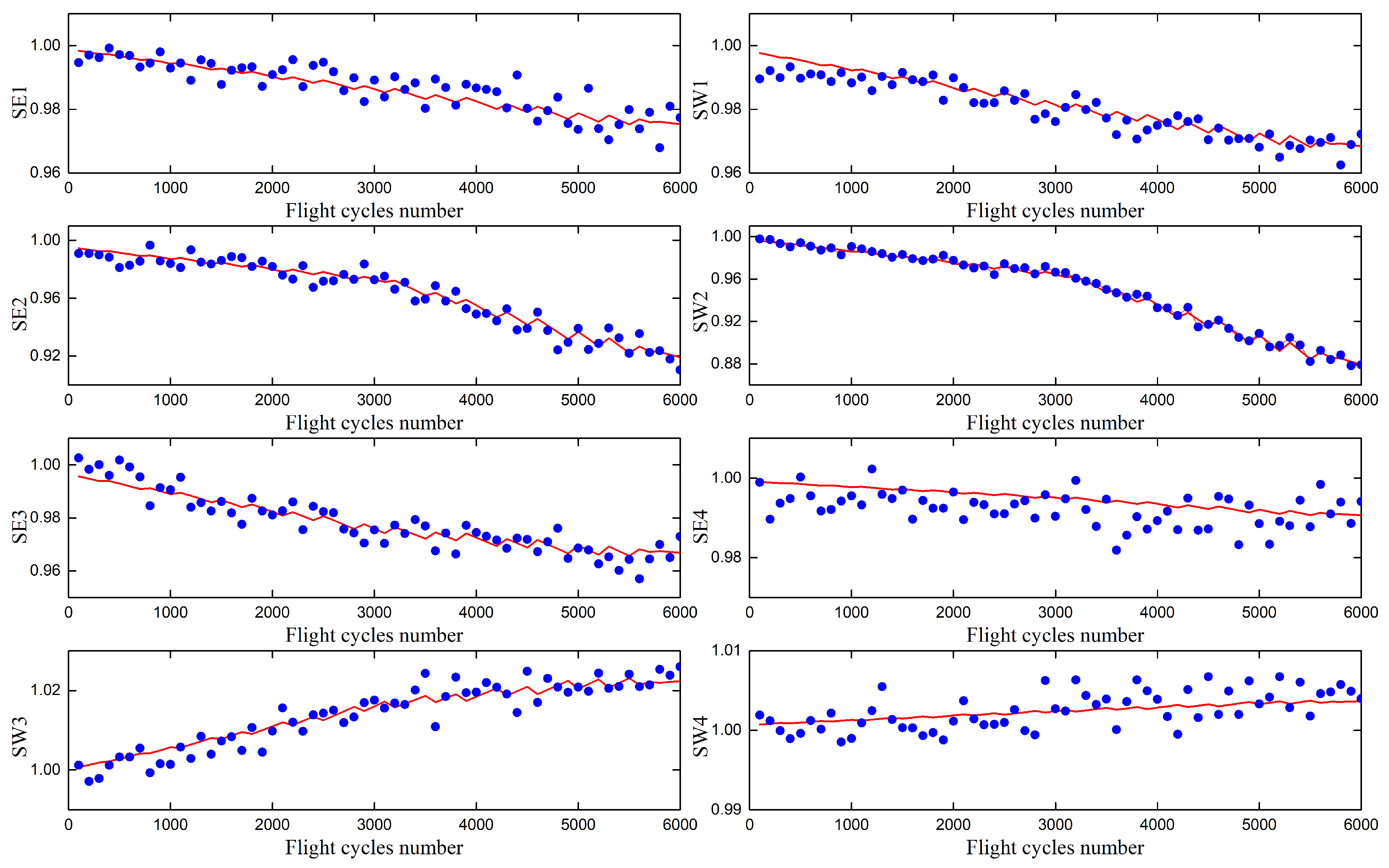
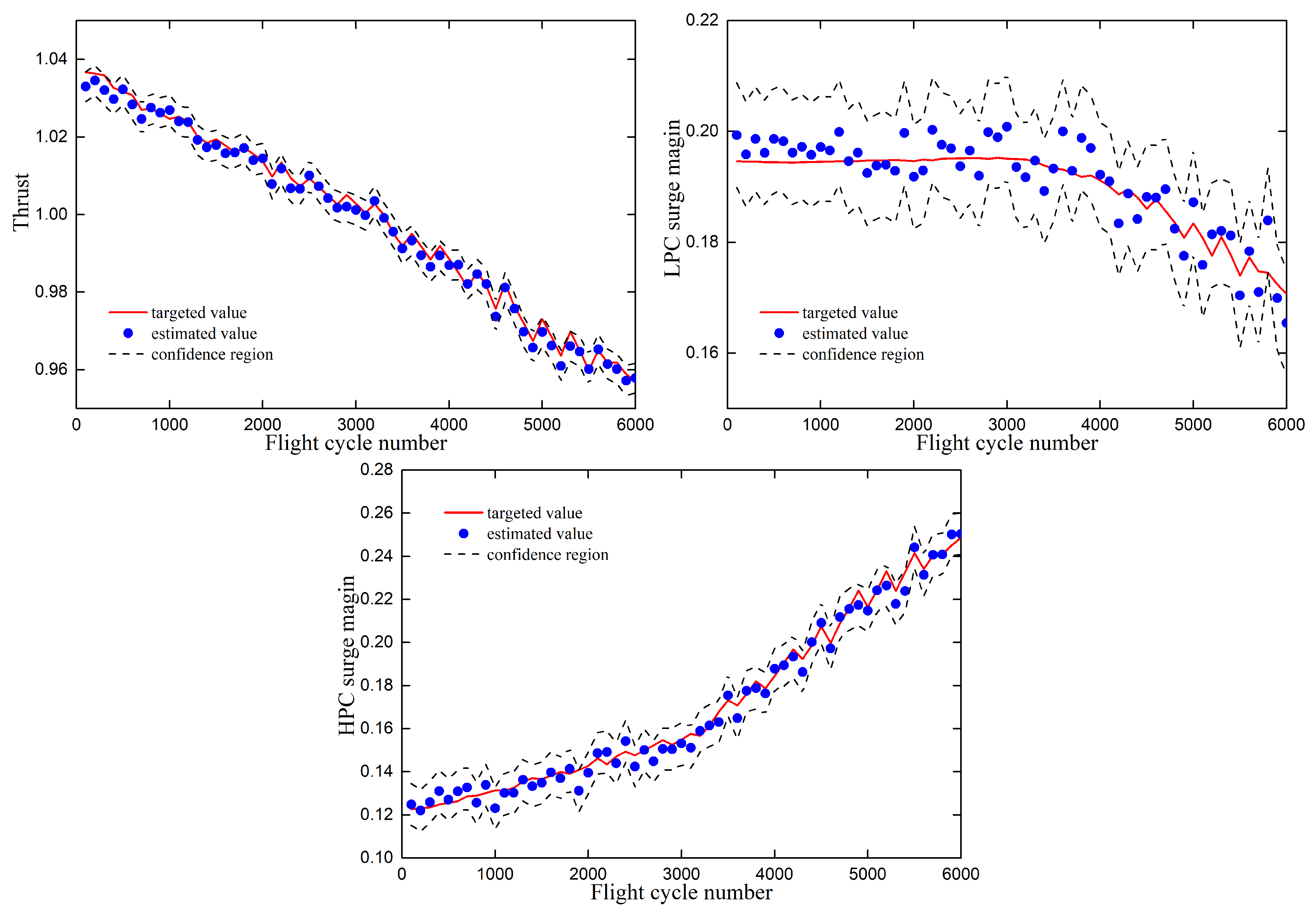
Figure 5 describes the health parameter degradation estimation of DKELMs algorithm with different flight cycle number. The general degradation degree of aircraft engine is assumed to be the linear interpolation with the percentages given in Table 5. In addition, degradation reference values also consider the periodic maintenance which results in the periodic fluctuation of reference values. It is clear that the values of health parameter estimated by DKELMs algorithm are consistent with the degradation reference values on the whole. The prediction result of thrust and surge margin is described in Figure 6. It can be seen that the values of thrust and surge margin estimated by DKELMs algorithm can generally reflect the change of target values. The confidence intervals corresponding to thrust, LPC surge margin and HPC surge marine are $\pm 0.0038$, $\pm 0.0094$ and $\pm 0.0097$ respectively. Thrust and LPC surge margin decrease with the increase of flight cycle number, which means the decline of component performance and reliability. Accurately predicting the degree of performance decline can provide effective technical guidance for depending maintenance.

5.2. Failure Patterns Recognition

In addition to gradual performance degradation, abrupt failure also often occurs in the service life of the aircraft engine, which would unexpectedly endanger the reliability and safety. Besides estimating the gradual degradation, failure diagnostics of aircraft engine also needs to be able to recognize the abrupt failure patterns, that is, to identify and classify the mode of abrupt failure according to observable parameters. It is assumed that the value range of each health parameter after abrupt failure is 30% to 100% of degradation after 3000 flight cycles. Because the magnitude of LPT efficiency change is too small, the change is almost submerged in the measurement noise. Therefore, abrupt failure of LPT efficiency is ignored and abrupt failure of other health parameters are considered in this subsection.

For single component failure, 10 failure patterns and corresponding fault health parameters are listed in

Table 8. Failure patterns of single component failure.

Pattern Code	Efficiency Failure	Flow Capacity Failure	Pattern Code	Efficiency Failure	Flow Capacity Failure
s1	LPC	-	s6	HPC	HPC
s2	-	LPC	s7	HPT	-
s3	LPC	LPC	s8	-	HPT
s4	HPC	-	s9	HPT	HPT
s5	-	HPC	s10	LPT	-

. The misclassification number of each single component failure pattern, through original KELM algorithm, proposed DKELMs algorithm and C-SVC algorithm are listed in

Table 9. Misclassification of each single component failure pattern through different algorithms.

Pattern Code	Number of Misclassification			Pattern Code	Number of Misclassification
	KELM	DKELMs	C-SVC		KELM	DKELMs	C-SVC
s1	22	25	19	s6	1	0	1
s2	26	20	28	s7	29	24	23
s3	15	7	28	s8	15	9	21
s4	7	5	8	s9	7	9	17
s5	1	0	3	s10	50	47	38
total	173	146	186

, where the testing samples are 200. Since all failure patterns are included in the training set, the error of all samples is considered when optimizing the loss function. When testing a characteristic failure pattern, it may occur that sometimes DKELMs algorithm has a greater misclassification number than the other two algorithms. Therefore, the accuracy of the algorithm should be measured by the total misclassification number. As can be seen from Table 9, the total misclassification number of proposed DKELMs algorithm is less than that of original KELM algorithm and C-SVC algorithm. The comprehensive performance comparison for single component failure recognition is listed in

Table 10. Comprehensive performance comparison for component failure recognition.

Failure Patterns	Algorithm	Correct Rate	Training Time/s	Testing Time/s
Single component failure	KELM	91.35%	3.1905	0.2325
	DKELMs	92.70%	0.4408	0.0976
	C-SVC	90.70%	0.9507	0.1178
Double components failure	KELM	89.95%	21.6213	0.9943
	DKELMs	91.05%	0.9743	0.2549
	C-SVC	90.21%	3.6765	2.7751

. It can be seen from the table that the correct rate of DKELMs algorithm is higher than KELM algorithm and C-SVC algorithm, and the training time and testing time are lower than the other two classification algorithms.

For concurrent component failure patterns, it is assumed that it only occurs on two adjacent components, that is, only three groups of components are considered, i.e., LPC & HPC, HPC & HPT, and HPT & LPT. Then, 21 failure patterns and fault health parameters of each pattern are listed in

Table 11. Failure patterns of concurrent component failure.

Pattern Code	Efficiency Failure	Flow Capacity Failure	Pattern Code	Efficiency Failure	Flow Capacity Failure
d1	LPC, HPC	-	d12	HPC, HPT	HPC
d2	HPC	LPC	d13	HPC	HPT
d3	LPC, HPC	LPC	d14	-	HPC, HPT
d4	LPC	HPC	d15	HPC	HPC, HPT
d5	-	LPC, HPC	d16	HPC, HPT	HPT
d6	LPC	LPC, HPC	d17	HPT	HPC, HPT
d7	LPC, HPC	HPC	d18	HPC, HPT	HPC, HPT
d8	HPC	LPC, HPC	d19	HPT, LPT	-
d9	LPC, HPC	LPC, HPC	d20	LPT	HPT
d10	HPC, HPT	-	d21	HPT, LPT	HPT
d11	HPT	HPC

.

Table 12. Misclassification of each concurrent component failure pattern through different algorithms.

Pattern Code	Number of Misclassification			Pattern Code	Number of Misclassification
	KELM	DKELMs	C-SVC		KELM	DKELMs	C-SVC
d1	31	13	11	d12	12	28	41
d2	11	6	5	d13	40	20	9
d3	15	16	12	d14	4	3	6
d4	39	15	17	d15	15	15	26
d5	14	13	3	d16	22	24	15
d6	14	29	22	d17	19	8	26
d7	23	41	38	d18	6	17	21
d8	17	10	25	d19	21	23	10
d9	10	24	43	d20	20	11	0
d10	24	13	25	d21	34	25	27
d11	31	22	29	total	422	376	411

lists the misclassification number of each concurrent component failure pattern, through original KELM algorithm, proposed DKELMs algorithm and C-SVC algorithm, and the testing samples are 200. It can be found that the proposed DKELMs has lower total misclassification number than original KELM algorithm and C-SVC algorithm. Table 10 lists the comprehensive performance comparison for concurrent component failure recognition. It is clear that the DKELMs algorithm has higher correct rate and lower training time and testing time than the other two classification algorithms for recognizing concurrent component failure as well.

6. Conclusions

The study of failure diagnostics is crucial for improving the safety and economic performance of aircraft engine, and KELM has attracted extensive attention in the field of failure diagnostics. Aiming for the disadvantages of original KELM algorithm such as excessive network size and high computational complexity, this paper proposes an innovative DKELMs algorithm. DKELMs makes the scale of the network controllable through distributed subnetworks. In addition, the fusion layer is designed for regression problems and classification problems respectively through likelihood probability and DS evidence theory. The accuracy of fusion result is similar to or higher than the original KELM, and the distributed architecture can effectively reduce the computational complexity. Simulations on benchmark datasets show that compared with KELM and SVM, the proposed algorithm can generate more compact network structure and higher learning speed for both regression problems and classified problems. Experiment results in estimating gradual component performance degradation and recognizing abrupt failure patterns show that DKELMs can effectively reduce training time and testing time while maintaining similar or even generating higher network accuracy practically.

References

- Jafari, S.; Nikolaidis, T. Meta-heuristic global optimization algorithms for aircraft engines modelling and controller design; A review, research challenges, and exploring the future. Prog. Aerosp. Sci. 2019, 104, 40–53. [Google Scholar] [CrossRef]
- Hao, Y.; Tao, Z. Design on Structural Test and Modeling of the Mounting Structure of a GTF Aircraft Engine. Appl. Mech. Mater. 2014, 607, 358–361. [Google Scholar] [CrossRef]
- Goebel, K.; Eklund, N.; Brunell, B. Rapid detection of faults for safety critical aircraft operation. In Proceedings of the 2004 IEEE Aerospace Conference Proceedings (IEEE Cat. No. 04TH8720), Big Sky, MT, USA, 6–13 March 2004; Volume 5, pp. 3372–3383. [Google Scholar]
- Wang, L.; Hu, J.; Huo, J.; Liu, Q.; Wei, B.; Tang, J.; Shi, X. Study on the cleaning mechanism of the fouling of the compressor blade. In Proceedings of the CSAA/IET International Conference on Aircraft Utility Systems (AUS 2018), Guiyang, China, 19–22 June 2018. [Google Scholar]
- Kumar, A.; Ensha, S.; Irvin, J.F.; Quinn, J. Liquid Metal Corrosion Fatigue (LMCF) Failure of Aircraft Engine Turbine Blades. J. Fail. Anal. Prev. 2018, 18, 939–947. [Google Scholar] [CrossRef]
- Gil-García, J.M.; Zubia, J.; Aranguren, G. Architecture for Measuring Blade Tip Clearance and Time of Arrival with Multiple Sensors in Airplane Engines. Int. J. Aerosp. Eng. 2018, 2018, 3756278. [Google Scholar] [CrossRef]
- Witek, L.; Bednarz, A.; Stachowicz, F. Fatigue analysis of compressor blade with simulated foreign object damage. Eng. Fail. Anal. 2015, 58, 229–237. [Google Scholar] [CrossRef]
- Rodriguez, L.F.; Botez, R.M. Generic new modeling technique for turbofan engine thrust. J. Propuls. Power 2013, 29, 1492–1495. [Google Scholar] [CrossRef]
- Tahan, M.; Tsoutsanis, E.; Muhammad, M.; Karim, Z.A. Performance-based health monitoring, diagnostics and prognostics for condition-based maintenance of gas turbines: A review. Appl. Energy 2017, 198, 122–144. [Google Scholar] [CrossRef] [Green Version]
- Hanachi, H.; Mechefske, C.; Liu, J.; Banerjee, A.; Chen, Y. Performance-Based Gas Turbine Health Monitoring, Diagnostics, and Prognostics: A Survey. IEEE Trans. Reliab. 2018, 67, 1340–1363. [Google Scholar] [CrossRef]
- Ahsan, S.; Lemma, T.; Muhammad, M. Prognosis of gas turbine remaining useful life using particle filter approach. Mater. Werkst. 2019, 50, 336–345. [Google Scholar] [CrossRef]
- Tan, Z.; Zhong, S.; Lin, L. A model learning strategy adapted to health assessment of multi-component systems. In Proceedings of the 2017 Prognostics and System Health Management Conference (PHM-Harbin), Harbin, China, 9–12 July 2017; pp. 1–7. [Google Scholar]
- Isermann, R. Model-based fault-detection and diagnosis–status and applications. Annu. Rev. Control 2005, 29, 71–85. [Google Scholar] [CrossRef]
- Liu, X.; Yuan, Y.; Shi, J.; Zhao, L. Adaptive modeling of aircraft engine performance degradation model based on the equilibrium manifold and expansion form. Proc. Inst. Mech. Eng. Part G J. Aerosp. Eng. 2014, 228, 1246–1272. [Google Scholar] [CrossRef]
- Kong, C. Review on advanced health monitoring methods for aero gas turbines using model based methods and artificial intelligent methods. Int. J. Aeronaut. Space Sci. 2014, 15, 123–137. [Google Scholar] [CrossRef]
- Loboda, I.; Pérez-Ruiz, J.L.; Yepifanov, S. A Benchmarking Analysis of a Data-Driven Gas Turbine Diagnostic Approach. In Proceedings of the ASME Turbo Expo 2018: Turbomachinery Technical Conference and Exposition, Oslo, Norway, 11–15 June 2018; p. V006T05A027. [Google Scholar]
- Antonakis, A.; Nikolaidis, T.; Pilidis, P. Multi-objective climb path optimization for aircraft/engine integration using Particle Swarm Optimization. Appl. Sci. 2017, 7, 469. [Google Scholar] [CrossRef]
- Lu, J.; Huang, J.; Lu, F. Sensor fault diagnosis for aero engine based on online sequential extreme learning machine with memory principle. Energies 2017, 10, 39. [Google Scholar] [CrossRef]
- Ordóñez, C.; Lasheras, F.S.; Roca-Pardiñas, J.; de Cos Juez, F.J. A hybrid ARIMA–SVM model for the study of the remaining useful life of aircraft engines. J. Comput. Appl. Math. 2019, 346, 184–191. [Google Scholar] [CrossRef]
- Zheng, C.; Liu, W.; Chen, B.; Gao, D.; Cheng, Y.; Yang, Y.; Zhang, X.; Li, S.; Huang, Z.; Peng, J. A Data-driven Approach for Remaining Useful Life Prediction of Aircraft Engines. In Proceedings of the 2018 21st International Conference on Intelligent Transportation Systems (ITSC), Maui, HI, USA, 4–7 November 2018; pp. 184–189. [Google Scholar]
- Skowron, M.; Wolkiewicz, M.; Orlowska-Kowalska, T.; Kowalski, C.T. Application of Self-Organizing Neural Networks to Electrical Fault Classification in Induction Motors. Appl. Sci. 2019, 9, 616. [Google Scholar] [CrossRef]
- Solarte-Pardo, B.; Hidalgo, D.; Yeh, S.S. Cutting Insert and Parameter Optimization for Turning Based on Artificial Neural Networks and a Genetic Algorithm. Appl. Sci. 2019, 9, 479. [Google Scholar] [CrossRef]
- Sansone, M.; Fusco, R.; Pepino, A.; Sansone, C. Electrocardiogram pattern recognition and analysis based on artificial neural networks and support vector machines: A review. J. Healthc. Eng. 2013, 4, 465–504. [Google Scholar] [CrossRef]
- Shukla, S.; Yadav, R.; Sharma, J.; Khare, S. Analysis of statistical features for fault detection in ball bearing. In Proceedings of the 2015 IEEE International Conference on Computational Intelligence and Computing Research (ICCIC), Madurai, India, 10–12 December 2015; pp. 1–7. [Google Scholar]
- Buscema, M. A brief overview and introduction to artificial neural networks. Subst. Use Misuse 2002, 37, 1093–1148. [Google Scholar] [CrossRef]
- Schmidhuber, J. Deep learning in neural networks: An overview. Neural Netw. 2015, 61, 85–117. [Google Scholar] [CrossRef] [Green Version]
- Huang, G.B.; Zhu, Q.Y.; Siew, C.K. Extreme learning machine: Theory and applications. Neurocomputing 2006, 70, 489–501. [Google Scholar] [CrossRef] [Green Version]
- Chorowski, J.; Wang, J.; Zurada, J.M. Review and performance comparison of SVM-and ELM-based classifiers. Neurocomputing 2014, 128, 507–516. [Google Scholar] [CrossRef]
- Lu, J.; Huang, J.; Lu, F. Time series prediction based on adaptive weight online sequential extreme learning machine. Appl. Sci. 2017, 7, 217. [Google Scholar] [CrossRef]
- You, C.X.; Huang, J.Q.; Lu, F. Recursive reduced kernel based extreme learning machine for aero-engine fault pattern recognition. Neurocomputing 2016, 214, 1038–1045. [Google Scholar] [CrossRef]
- Huang, G.B.; Zhou, H.; Ding, X.; Zhang, R. Extreme learning machine for regression and multiclass classification. IEEE Trans. Syst. Man Cybern. Part B Cybern. 2012, 42, 513–529. [Google Scholar] [CrossRef]
- Li, K.; Su, L.; Wu, J.; Wang, H.; Chen, P. A rolling bearing fault diagnosis method based on variational mode decomposition and an improved kernel extreme learning machine. Appl. Sci. 2017, 7, 1004. [Google Scholar] [CrossRef]
- Fu, H.; Vong, C.M.; Wong, P.K.; Yang, Z. Fast detection of impact location using kernel extreme learning machine. Neural Comput. Appl. 2016, 27, 121–130. [Google Scholar] [CrossRef]
- Volponi, A.; Simon, D.L. Enhanced Self Tuning On-Board Real-Time Model (Estorm) for Aircraft Engine Performance Health Tracking; NASA: Washington, DC, USA, 2008.
- Fill, J.A.; Fishkind, D.E. The Moore–Penrose Generalized Inverse for Sums of Matrices. Siam J. Matrix Anal. Appl. 2000, 21, 629–635. [Google Scholar] [CrossRef]
- Duan, Y.; Cai, Y.; Wang, Z.; Deng, X. A novel network security risk assessment approach by combining subjective and objective weights under uncertainty. Appl. Sci. 2018, 8, 428. [Google Scholar] [CrossRef]
- Dheeru, D.; Taniskidou, E.K. UCI Machine Learning Repository; University of California: Irvine, CA, USA, 2017. [Google Scholar]
- Chang, C.C.; Lin, C.J. LIBSVM: A library for support vector machines. ACM Trans. Intell. Syst. Technol. 2011, 2, 27:1–27:27. Available online: http://www.csie.ntu.edu.tw/~cjlin/libsvm (accessed on 11 February 2019). [CrossRef]
- Ying, Z.; Keong, K. Fast leave-one-out evaluation for dynamic gene selection. Soft Comput. 2006, 10, 346–350. [Google Scholar] [CrossRef]
- Chatterjee, S.; Litt, J. Online model parameter estimation of jet engine degradation for autonomous propulsion control. In Proceedings of the AIAA Guidance, Navigation, and Control Conference and Exhibit, Austin, TX, USA, 12 August 2003; p. 5425. [Google Scholar]
- DeCastro, J.; Litt, J.; Frederick, D. A modular aero-propulsion system simulation of a large commercial aircraft engine. In Proceedings of the 44th AIAA/ASME/SAE/ASEE Joint Propulsion Conference & Exhibit, Hartford, CT, USA, 21–23 July 2008; p. 4579. [Google Scholar]
Figure 1.
Network structure of the original Kernel Extreme Learning Machines (KELM) algorithm.
Figure 2.
Distributed framework of proposed distributed kernel extreme learning machines (DKELMs) algorithm.
Figure 3.
Comparison on and testing time in regression benchmark datasets. (Red, blue and green respectively represent the original KELM, n-SVR and DKELMs algorithms. Different legend shapes represent different datasets).
Figure 4.
Comparison on correct rate and testing time in classification benchmark datasets. (Red, blue and green respectively represent the original KELM, C-SVC and DKELMs algorithms. Different legend shapes represent different datasets).
Figure 5.
Health parameters degeneration estimation after different flight cycles through DKELMs algorithm (the line denotes target value and the point denotes estimated value).
Figure 6.
Prediction results for thrust and surge margins.