Plant Disease Diagnosis for Smart Phone Applications with Extensible Set of Diseases


Computer Science and Engineering Department, University of Thessaly, 41110 Larissa, Greece
Appl. Sci. 2019, 9(9), 1952; https://0-doi-org.brum.beds.ac.uk/10.3390/app9091952
Submission received: 4 March 2019
/
Revised: 25 April 2019
/
Accepted: 10 May 2019
/
Published: 13 May 2019
(This article belongs to the Section Electrical, Electronics and Communications Engineering)
Abstract
:Featured Application
A low complexity image processing and a new classification method are proposed in this paper. These methods can be employed by plant disease diagnosis applications implemented on smart phones. The supported set of diseases can be extended by the end user.
Abstract
A plant disease diagnosis method that can be implemented with the resources of a mobile phone application, that does not have to be connected to a remote server, is presented and evaluated on citrus diseases. It can be used both by amateur gardeners and by professional agriculturists for early detection of diseases. The features used are extracted from photographs of plant parts like leaves or fruits and include the color, the relative area and the number of the lesion spots. These classification features, along with additional information like weather metadata, form disease signatures that can be easily defined by the end user (e.g., an agronomist). These signatures are based on the statistical processing of a small number of representative training photographs. The extracted features of a test photograph are compared against the disease signatures in order to select the most likely disease. An important advantage of the proposed approach is that the diagnosis does not depend on the orientation, the scale or the resolution of the photograph. The experiments have been conducted under several light exposure conditions. The accuracy was experimentally measured between 70% and 99%. An acceptable accuracy higher than 90% can be achieved in most of the cases since the lesion spots can recognized interactively with high precision.
1. Introduction
Image processing and machine vision have been widely used in monitoring plants, harvesting, and other stages of plant growing. For example, Liu et al. [1] presented a review about the use of machine vision systems in identifying common invertebrates on crops, such as butterflies, locusts, snails and slugs. Image processing is usually combined with artificial intelligence like neural networks to detect mature fruits [2,3,4,5]. In these cases, the accuracy ranges between 60% and 100% depending on the type of fruit and other conditions. Crop monitoring is another domain where machine vision has been adopted (e.g., for production monitoring [6], the detection of diseases, or insect invasion) [7]. Unmanned aerial vehicles (UAVs) have been recently employed for the monitoring of large rural areas by analyzing images captured from a high altitude. Ballesteros et al. [8] discussed several UAV approaches based on red-green-blue (RGB), near infrared camera and other sensors. Calderon et al. [9] used a multispectral image and thermal view from an UAV to detect if opium poppy was affected by downy mildew. Common image segmentation techniques and classification methods like neural networks, decision trees, support vector machines (SVM), etc., have been used in both the diagnosis of plant and human diseases (e.g., skin disorders) [10].
The early detection of plant diseases is necessary for effective control reassuring that the financial cost and the environmental impact of their treatment will be minimized. If plant diseases are not treated in their early stages, the production cost can be significantly increased since the disease can propagate to the whole crop. The traditional way is to hire professional agriculturists who monitor the plants, but this may not always be possible for farms set in isolated rural areas. Moreover, the cost may not be affordable for smaller farmers. Remote monitoring and automation offered by precision agriculture solutions can reduce the cost and offer efficient protection. The initial detection of a disease can be based on machine vision and image processing that will generate an alert if its symptoms are recognized. Molecular analyses have a higher cost but may be carried out later if a plant disease has to be formally confirmed.
The plant disease diagnosis can be based on various symptoms as described in [11,12]. Symptoms can often be grouped as: (a) underdevelopment of tissues or organs (short internodes, underdeveloped roots, malformed leaves, lack of chlorophyll, fruits and flowers that do not develop), (b) overdevelopment of plant parts like tissues or organs, (c) necrosis of plant parts (wilts, shoot or leaf blights, leaf spots, fruit rots) and (d) alternations like mosaic patterns and altered coloration in leaves and flowers.
The progression of the disease symptoms can vary significantly. Biotic agents affect the speed of the symptom progression. There are primary and secondary symptoms of a disease. For example, a primary symptom can be the root decay of a tree while the secondary symptom can be the tree toppling over. Secondary invaders that attack the tree in the later stages of a disease may obscure the original disease symptoms making the diagnosis more complicated. Other facts like improper herbicide usage can cause similar symptoms to spots that are present as a result of an infectious agent. Nevertheless, the symptoms caused by herbicide injury appear suddenly and no progression is observed. The spots may also follow spray patterns of the herbicide. Herbicides can also cause leaf distortion which may be confused with viral diseases. However, the new leaves are free of symptoms, indicating a lack of symptom progression. More than one problem or pathogen infecting the plant can be present. In this case, the symptoms may significantly differ from that of the individual pathogens when they act alone.
Several image processing techniques have been presented in the literature for plant disease recognition. Reviews of image processing techniques in visible light including classification, real-time monitoring and neural networks can be found in [13,14]. Image segmentation in the International Commission on Illumination (CIE) L*a*b color space, followed by a Gabor filter to form an input to the neural network that achieves a disease recognition with 91% accuracy, was presented by Kulkarni and Patil in [15]. Carmago and Smith [16] applied image processing for disease identification based on shape, texture fractal dimension, lacunarity, dispersion, gray levels, gray histogram discrimination and Fourier descriptors. Mohanty et al. [17] evaluated two deep convolutional neural networks (AlexNet, GoogLeNet) using thousands of images as a training set with an accuracy higher than 98%. Customized disease detection solutions for specific plants have also been presented (e.g., by Lai et al. for corn diseases [18], Schaad et al. [19] for citrus pathogens, etc.).
Sankaran et al. reviewed in [20] some image processing techniques and molecular tests. Molecular tests like the polymerase chain reaction (PCR) technique can be applied as described by Schaad and Frederick in [19]. The sensitivity of the PCR depends on the amount of the microorganism that is tested.
There are not many references in the literature for smart phone applications developed for plant disease diagnosis. A mobile client–server architecture for leaf disease detection and diagnosis using a novel combination of a Gabor wavelet transform and gray level co-occurrence matrix, is proposed in [21]. A diseased patch is processed to extract a multi-resolution and multi-direction feature vector. The mobile client captures and pre-processes the leaf image, segments diseased patches in it and transmits the results to the pathology server which performs feature extraction and classification using k-nearest neighbor with 93% accuracy. In [22], it is stated that the use of image processing can leverage early detection of diseases but they perform poorly under real field conditions using mobile devices. An image processing algorithm based on candidate hot-spot detection, in combination with statistical inference methods, is proposed for disease identification in wild conditions. Seven mobile devices were used to capture and analyze more than 3500 images displaying wheat diseases (Septoria, rust and tan spot). The measured “Area under the Receiver Operating Characteristic–ROC–Curve” metrics were higher than 0.80 for all the analyzed diseases. A heuristic method based either on graphical representation or a step-by-step descriptive method, was used for plant disease recognition by Abu-Naser et al. in [23]. A set of questions are answered by the user in the step-by-step procedure while in the graphical representation, the user compares photographs of the closest disease cases. This approach requires internet connection. The application Purdue Plant Doctor [24] is offered in different versions for each plant type for iOS or Android platforms. It is also based on questionnaire and decision trees in order to diagnose a disease. A similar application to the one presented in this paper is Plant Doctor offered by Plantix [25]. It is an expert system trained to recognize a large number of diseases. It can communicate with a remote database for higher accuracy.
The plant disease recognition method described in this paper is targeted for mobile phone applications. The term “disease” in this paper refers to any situation that can damage a plant including pathogens, biotic agents, nutritional deficiency, pollution, harmful weather conditions, etc. The proposed method is based on the extraction of various features from a photograph of a plant part. These features include the number of spots, their relative area, the spot, leaf and halo color, weather conditions, etc. Absolute lesion dimensions can be easily estimated and taken into account, although only relative dimensions are used here. The plant part can be a leaf, fruit, branch, root, etc. Each one of the extracted feature values is compared with wide and narrow ranges defined in the signature of a specific disease. A different grade is given if a feature value resides within the narrow or the wider range of the corresponding disease feature, otherwise a zero grade is given. The weighted sum of the grades assigned for each feature ranks the likelihood of a specific disease. This classification method can be characterized as fuzzy-like clustering with discrete ranks assigned to each cluster (disease). The novelty in the employed classification method stems from the combination of the specific features used (e.g., the similarity of the extracted histograms is determined by the beginning, the ending and the peak of the lobes) and the comparison of each feature value with multiple ranges. The simplicity of the employed classification method allows the full implementation of the proposed method on a smart phone that does not have to be connected to a remote server as is the case, for example, in [21]. The simplicity is also necessary for the extensibility of the supported set of diseases by the administrator of the application instead of its developer, without having to train the system with numerous images and image patches. As will be demonstrated by the experimental results and the comparison with other popular classification algorithms, the selected classification method achieves very good results despite its simplicity.
The disease signature can be defined by an end user that does need to have access to the application source code and does not have to be familiar with its architecture either. This makes the application extensible since it is capable of supporting an unlimited number of plants and diseases. A relatively small training set consisting of representative photographs can be used to define a disease signature. The recognition accuracy may be low if a very small number of training photographs are used due to extremely different environmental conditions or varieties of the same plant that may appear in a new photograph. However, a small training set may be adequate for the recognition of diseases that appear in the same geographical region where the training was carried out. The missing information due to the small training set is compensated by the large number of features used in the disease signatures. Although the training set size scales up with the size of the test set, it is expected that a limited number of training photographs will be sufficient to cover all the cases. The recognition algorithm is fast and does not consume a large number of mobile phone resources.
The approach presented in this paper is an extension of the application described by the author in [26,27,28] (see Video S1) where a minimal set of features used for disease recognition was defined. Some initial experiments have been performed in these papers using grape, peach, or citrus leaves. The approach presented here differs from our previous work in the following: (a) the disease signatures are extended (the color features of the halo around the spots are taken into consideration), (b) the disease recognition method is described in detail, (c) automatic segmentation methods (for background separation and lesion spot recognition) are introduced and evaluated, (d) the extensibility of the system is assisted by tools that automate the disease signature definition, (e) extensive experimentation with citrus diseases is carried out under different light exposure using photographs of upper or lower leaf surface and orange fruits, (f) color normalization issues are discussed to minimize the effect of different light exposure, (g) the specific features used in the proposed classification scheme are tested with a number of popular classification algorithms (decision trees, random forests, neural networks, etc.) and the results are compared with the ones achieved by the proposed classification scheme.
2. Materials and Methods
The disease recognition method described in this paper is based on symptoms appearing on any part of the plant. This part can be the upper or lower surface of a leaf, fruit, branch, or root, etc. The proposed method attempts to locate the diseased region of this plant part which may be lesion spots or simply regions with a different color, indicating infection by a disease. It is assumed here that the normal plant part has a distinct color and the same holds for the spots. Each spot may be surrounded by a halo as is the case with several diseases. For example, the Diaporthe citri saprophyte melanose in citrus trees or the oomycete parasites of downy mildew in grape leaves are identified by several small black spots or larger brown spots, respectively, without a halo (in most of cases). Alternaria citri (A. citri) in citrus trees can be identified by a small number of large dark leaf spots surrounded by a thick yellow halo that is brighter than the green color of the normal leaf. Similarly, the colonization of the citrus leaves by the fungus anthracnose can be recognized by several dark spots surrounded by a brighter than the normal thin halo (or vice versa). In cases like nutrient deficiency or Esca, several brighter yellow colored regions appear on the whole leaf that can also be considered as spots. The user has to identify if the spots (i.e., the diseased plant parts are brighter or darker than the normal plant part).
In the present version of the application it is assumed that, a single leaf or fruit has been captured on a much brighter background to make easier its distinction. Although this may seem restrictive, the brighter background can be created simply by placing the examined part of the plant on a sheet of paper or a marble bench. The background could also be much darker than the analyzed plant part. In both cases, if a pixel of the analyzed plant part has a similar color to the background it may be misinterpreted as background, but this can also be easily handled by taking into consideration the perimeter of the plant part. In many cases the plant part (e.g., the fruit) may have a much darker or brighter color than the leaves behind it. For example, this is the case when focus is given on a citrus fruit having dark green leaves behind it. This can be handled by the supported background separation algorithm without any modification. Another way to avoid the use of a complicated background separation algorithm is to focus on the lesion and take a photograph so close that only the plant part appears with no background at all. Finally, the plant disease diagnosis method presented in this paper can also be tested on photographs that display multiple leaves or fruits. For example, photographs taken close to a citrus tree displaying multiple leaves or fruits with no background can be used. Of course, the details of the lesions will be hidden in this case and different disease signatures based on representative images of this type will have to be defined. In future versions of the developed application more sophisticated background separation algorithms may be incorporated, as long as they are not too complicated, in order to be supported by the resources of a mobile phone.
The plant disease diagnosis application presented in this paper was exhaustively tested on citrus diseases and their symptoms on the leaves and the fruits. Three groups of photographs were used. The first group (A) consists of leaves captured under direct sunlight. The second group (B) includes the same leaves photographed under a canopy. The third group (C) consists of orange fruit photographs captured under various environmental conditions (sunlight, cloudy day, shade). In the photographs that were taken under direct sunlight, the colors of the various areas are more distinctive but the shade of the leaf can be confused with a spot. If the photographs are taken under a canopy no intense shadow appears, but the contrast between the colors is reduced. Five citrus diseases had to be distinguished using the leaf photographs (Alternaria, anthracnose, citrus chlorotic dwarf virus (CCDV), nutrient deficiency, melanose) and four using the photographs displaying fruits (brown rot, fruit split, melanose, Septoria). About half of the tested photographs were captured from private citrus trees (lemon, orange, tangerine) in the Achaia region (Greece) and the rest from citrus trees in Lesvos island (Greece). These regions have a distinct climate but the appearance of the examined diseases is not significantly different. Another set of photographs displaying pear leaves with 4 diseases (fire blight, pear scab, Mycosphaerella, powdery mildew) have been recently tested in various color spaces using linear dynamic range expansion (DRE). These photographs have been retrieved from pear trees in the Achaia region. The specific disease displayed in each photograph was identified by a professional agronomist and this diagnosis served as ground truth for the evaluation of the developed classification system.
The number of test photographs used per disease ranges between 22 and 56 and the number of these photographs that were used for training, ranges between 6 and 8. The fraction of the test set used for training, ranges between 6/56 = 10.7% and 8/22 = 36.4%. The test photographs were captured using ordinary smart phone cameras with resolution ranging from 5 MPixels (Lumia 550, Microsoft, One Microsoft Way, Redmond, Washington, U.S.) to 23 MPixels (Sony Xperia XA1, 1-7-1 Konan Minato-ku, Tokyo, 108-0075 Japan). These photographs were resized by the developed application to 1024 × 576 pixels for high speed operation since the employed image processing and classification methods do not require an excessively high resolution. The photographs were processed in red-green-blue (RGB) format although different formats have also been tested for color normalization as will be explained in the following sections.
2.1. Image Processing Method and Feature Extraction
In this section, the methods for the extraction of the various features used by the classification method are discussed. First of all, the background and the photograph pixels belonging to the plant part have to be separated. As already mentioned, it is assumed for convenience that the plant part has been photographed with a background much brighter or darker than the examined plant part. This prerequisite would not be necessary if, for example, a citrus fruit had to be photographed on the tree since its yellow color would make it easy to distinguish it from the green leaves. However, isolating a single leaf of a tree in a photograph would be much harder requiring an image processing technique potentially more complicated than, for example, the segmentation technique used for the rest of the image regions. Two methods are supported for the identification of the white background. In the first, (background separation method 1, BSM1), the gray version of the photograph is used and the pixels with a gray level higher than a threshold Bg are assumed to be the background. In the second method (BSM2) it is assumed that the three color levels of the RGB background pixels are very close and have a relatively high value (e.g., >200). The pure white color is generated if R = 255, G = 255 and B = 255. However, if a photograph is taken under a shadow, the background is slightly darker and these color levels are lower but even in this case they are approximately equal. The BSM2, marks a pixel i with color levels: Ri, Gi, Bi as the background if all the following conditions hold:
The precise values of the constants c1 and c2 are not critical. For example, selecting c1 = 200 and c2 = 30 worked satisfactorily for all the tested cases. Similarly, if the background is darker (black for simplicity) compared to the examined plant part, it could be identified if its pixel’s gray or color levels are close to 0. The drawback of these low complexity background separation methods is that a region of the plant part can be confused and recognized as the background if its color is similar to the color of the background. If the confused region does not reach the boundary of the plant part, the ambiguity of whether it belongs to the plant part or the background can be easily solved by checking if it exists within the perimeter of the examined leaf or fruit.
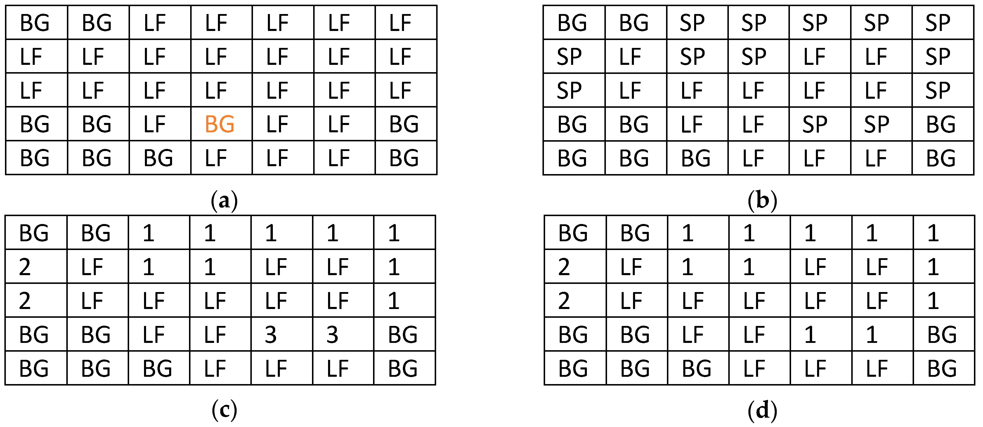
Assuming that the background (BG) pixels have been identified and the rest of the pixels are marked as normal plant part (LF), then a portion of the image may be represented as shown in Figure 1a. Each cell in Figure 1 corresponds to a single pixel. If a pixel internal to the plant part region has been mistakably interpreted as background (as the central red BG pixel of Figure 1a) then the following check can (in most of the cases) reveal the error and correct it: all the pixels up to the image border, in each one of the four directions (up, down, left, right) are examined. In each one of these directions, if only LF or both BG and LF pixels are found, then it is likely that this pixel belongs to the normal plant part (e.g., leaf). The correction of such BG pixels can be performed with higher confidence if the pixels of the four diagonals are also examined in the same way. A different method would first map the plant part perimeter and then check the coordinates of a pixel to verify if it is located within this perimeter. After this first step, let us assume that the spot pixels (SP) have been identified as shown in Figure 1b. The area of the spots (As) as a fraction of the overall leaf area can simply be estimated as the ratio of the number of spot pixels to the number of both the spot and the leaf pixels. True dimensions can also be estimated as described in [28] if the distance of the camera from the plant part is known. However, knowing absolute dimensions is not very useful since it is more important to know the relative leaf area that has been infected.
The number of spots can be estimated as follows. The image matrix of Figure 1b is scanned row by row, top-down and from left to right. When a spot pixel is found it is assigned with an identifier. The neighboring top-left, top, top-right and the adjacent pixel on the left that have already been visited are examined to see if they are spot pixels. If at least one of them is indeed a spot pixel, its identity is also given to the current pixel otherwise it is assigned with the higher identity that has already been used, incremented by 1. In this way, all pixels belonging to the same spot are marked with the same identity and the highest identity used indicates the number of spots. The result of this procedure is shown in Figure 1c. However, as can be seen from Figure 1c it is possible that adjacent spot pixels can be assigned with different identities (the spot No. 3 at the fourth row is adjacent to the spot No. 1). For this reason, it is necessary to iteratively check if there are adjacent spots with different identity. In this case, they should be merged (assigned with the lowest identity of the two) and the rest of the spots should be renumbered. This iterative procedure stops if no further modifications are needed.
The final map (henceforth this matrix will be called BNS) shown in Figure 1d can be used to estimate the number of spots (Ns) which is the maximum identity used when the numbering is finalized. The pixels that are mapped to a normal plant part like LF in Figure 1 can be used to estimate the average gray level of the normal leaf (Gl). Similarly, the gray level of the lesion spots (Gs) and the halo (Gh) are estimated by the spot and the halo pixels. Additional features related with the weather conditions like the average moisture (Md), and minimum (Tn) and maximum (Tx) temperature, are retrieved by weather metadata available on the internet as will be explained in the next section. If a spot consists of a very small number of pixels it can be ignored since it may be a result of noise.
Three ways are supported for the identification of the spot pixels on a leaf. The first way (spot separation method 1, SSM1) uses the representation of the image in the gray scale and focuses on the leaf pixels. The average gray level Gav of all the leaf pixels is estimated and then, the pixels that their gray level deviates from Gav by more than a threshold Th, are assumed to be lesion spots. Formally, it can be stated that each pixel BNS(i,j) in the matrix shown in Figure 1b can be defined by its corresponding one in the gray image Gr(i,j) under the following conditions that hold if the background is white:
If the lesion is brighter than the normal leaf, the user sets the flag “Invert” as will be shown in the following sections. The user also defines manually the thresholds Bg and Th. Although it may be frustrating for a user to calibrate in real-time these parameters, this method is quite accurate in mapping correctly the leaf, spot and background regions. The user can interactively verify that he has selected appropriate values for the Bg and Th parameters by comparing the segmented with the original image.
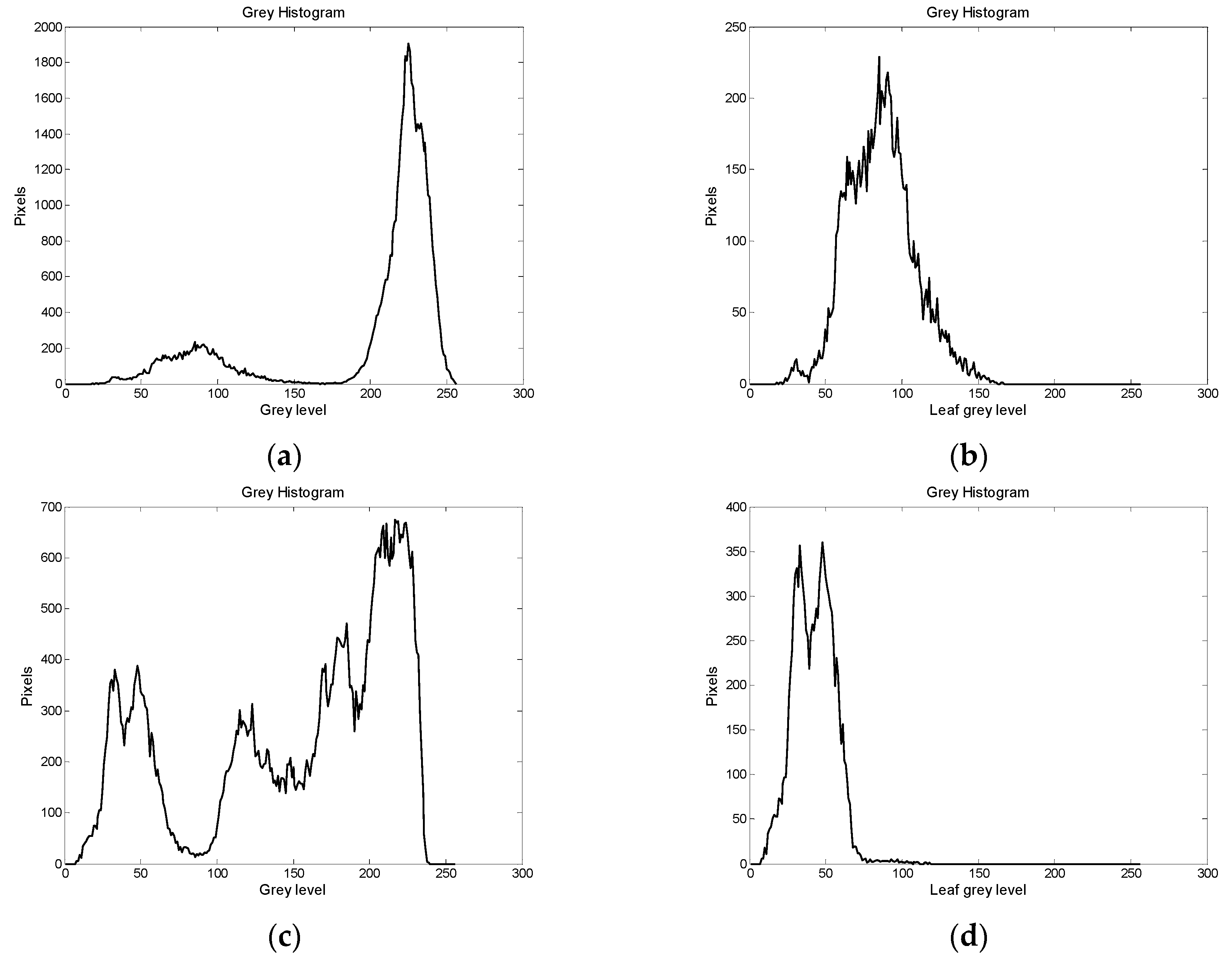
In the spot separation method 2 (SSM2), BSM2 is used for the background separation but the threshold Th is constant (Th = 30), since it was experimentally observed that this value is appropriate for most of the cases. In the SSM3, again BSM2 is used for background separation, but the spots are separated from the normal plant part using the gray histogram as shown in Figure 2.
The gray or color histograms used in this application are defined as follows: Each position on the horizontal axis is the gray or color level. The value of the histogram in this position denotes the number of pixels that have this specific color level. In Figure 2a,c, the gray histogram has been generated by all the pixels of each image with citrus leaves infected by Alternaria citri or Diaporthe citri (melanose), respectively. Figure 2b shows the gray histogram generated only by the pixels of the leaf used in Figure 2a (not the background). In this case, the background pixels have been separated using BSM1. Similarly, Figure 2d shows the gray histogram generated only by the pixels of the leaf used in Figure 2c and BSM2 is used in this case. In both cases, the large lobe in the histograms of the full image, that starts above the position c1 = 100, corresponds to the white or light gray background and the lower lobes correspond to the leaf and spot pixels. In SSM3 these areas are separated by estimating a local minimum Tm. In Figure 2d, the local minimum is clearly the position Tm = 50. However, selecting the local minimum in Figure 2b is not obvious. In this case, there is a minimum at the position 45 and another local minimum approximately at the position 70. Several other local minima can be found but they are not taken into consideration since they are estimated in a window of 20–30 successive positions to avoid noise. The selection between the values 45 or 70 for the threshold Tm depends on how the start of the lobe is defined. If it is assumed that a lobe starts when the histogram value exceeds a minimum but not zero value, then Tm = 70 may be selected. In any case, the leaf pixels with gray level higher than the Tm value are assumed to be normal leaf and the rest to be lesion spots if the lesion is darker than the normal leaf. If the lesion is brighter than the normal leaf, then its spots are those with a gray level higher than Tm.
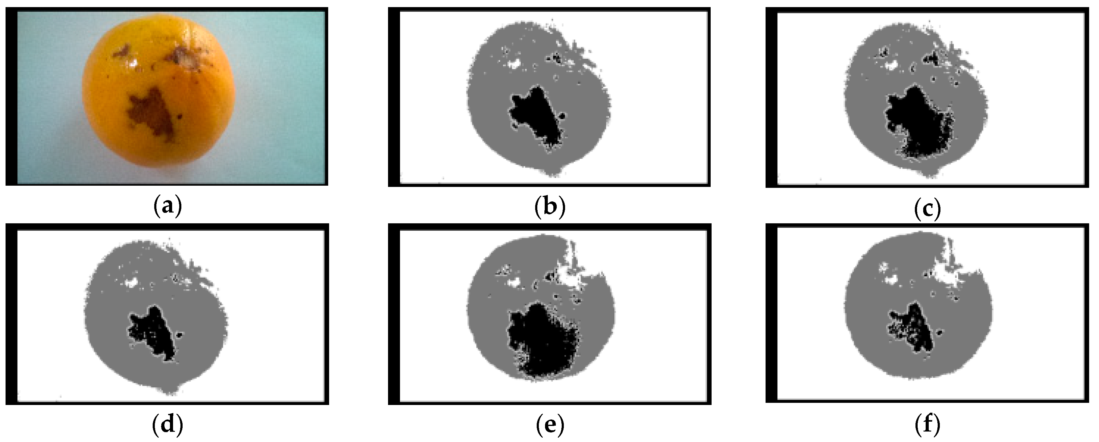
The efficiency of SSM1, SSM2 and SSM3 is demonstrated with two examples in Figure 3 and Figure 4. Figure 3a shows the upper surface of a leaf infected by the fungus Diaporthe citri of melanose. If SSM1 is used, then setting Th = 20 leads to the most precise spot mapping as shown in Figure 3b. If Th = 10, a part of the normal leaf area is marked as lesion (Figure 3c), while if Th = 30 some spots are not recognized (Figure 3d). SSM2 leads to accurate spot mapping as shown in Figure 3e. However, SSM3 fails to recognize several spots. In Figure 4a an orange that is infected by the dematiaceous hyphomycete of Pseudocercospora angolensis is displayed. Now, if SS1 is used, the optimal value for Th is 30 (Figure 4b). Again selecting a lower Th value marks more normal fruit area as lesion (Figure 4c), while selecting a higher Th value does not recognize all the lesion spot areas (Figure 4d). In this case, SSM3 achieves a better spot recognition than SSM2. Although selecting the preferable SSM may seem complicated, the user is assisted interactively by the developed application to choose the appropriate SSM.
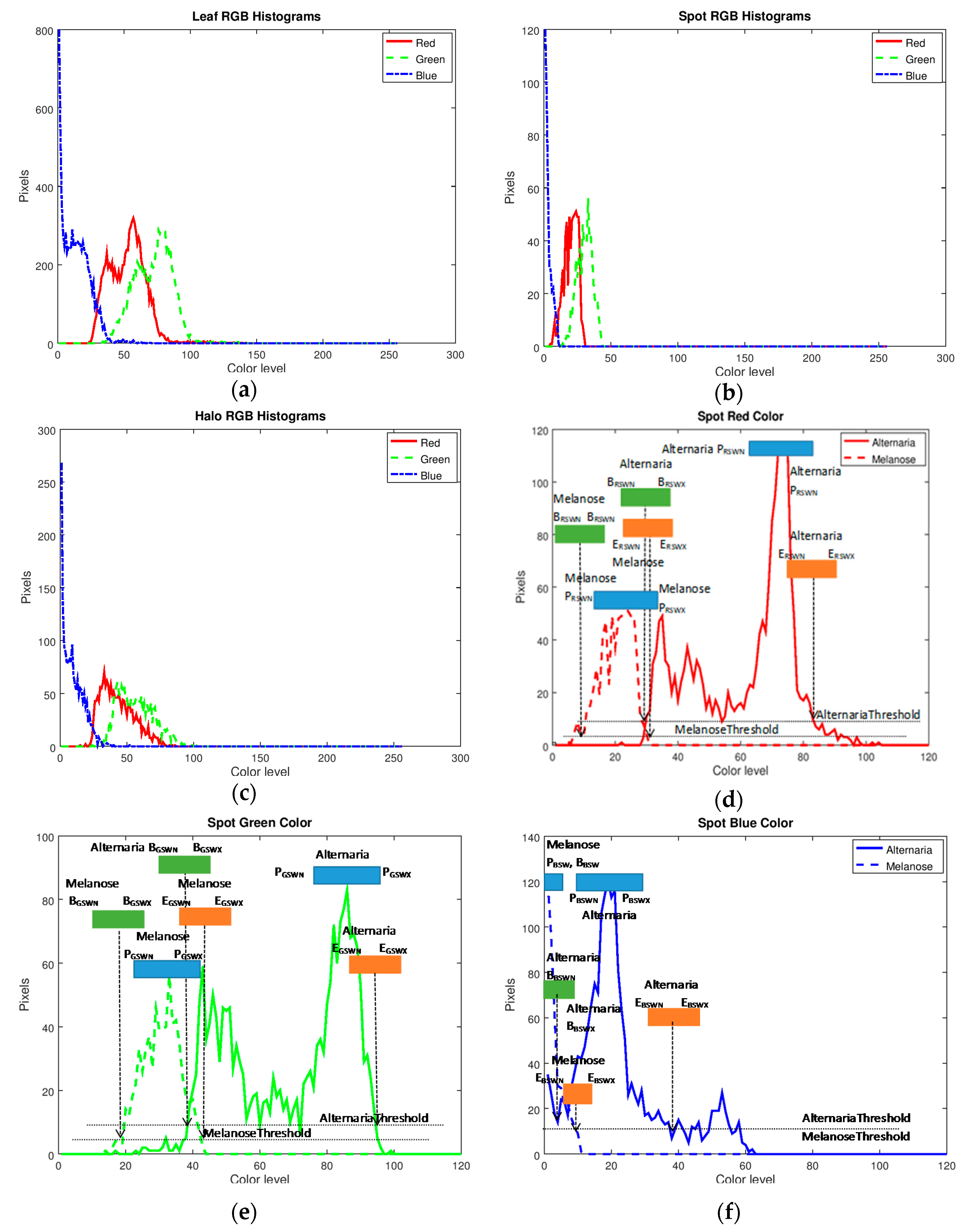
Three triplets of color histograms are required for the extraction of the rest of the features used in the employed classification method. These are the RGB histograms of the spots, the normal plant part and the halo around the spots. Figure 5a–c shows these histograms for the citrus leaf of Figure 3a. The halo histogram displayed in Figure 5c has been derived by a zone of 3 pixels wide (a configurable parameter) around each spot. Since there is no halo around the spots, it consists in this case mainly of normal leaf pixels or spot pixels that failed to be identified.
The shape of these histograms is not the same in different diseases. It may also be slightly different for photographs showing different leaves, infected by the same disease, if they are captured under different light exposure or at different stages of the disease progression. Some basic rules can be followed to avoid extreme environmental condition variations like using photographs that have been taken under a canopy to avoid intense shades, selecting cloudy rather than sunny days to take the photographs, etc. In order to moderate the symptom diversity caused by the variety of these conditions, several signatures are defined in the developed application corresponding to different progression levels of a disease. For example, grapevine downy mildew caused by the agent Plasmopara viticola appears initially as a brighter lesion than the normal grape leaves that turns to brown spots in later stages. Two disease signatures can be defined for these two stages of the same disease.
Moreover, a color normalization technique has been employed to moderate the light exposure variations. The gray level of the normal plant part is used as a reference to adjust the brightness of the lesion and the spots. More specifically, the average gray level of the normal plant part is estimated by the training photographs during the signature definition. When a new photograph is examined, the new gray level GN of the normal plant part is also estimated and the signed difference , is added to all the color planes (R, G, B) of the lesion and the halo pixels before the analysis takes place. This color normalization technique has been initially tested in the skin disorder diagnosis application presented in [27], that is based on the same image segmentation and classification method.
Gray images are often normalized through linear DRE, using the following formula:
where gnew, gold are the new and the old gray level of a specific pixel and gmin, gmax are the minimum and maximum gray level in the region of interest. However, if this color stretching is applied independently to the basic colors of an RGB image, it will be distorted. Despite this distortion, we have attempted to apply a similar type of normalization as the one described by Equation (3) to the value component of hue-saturation-value (HSV), or the lightness component of hue-saturation-lightness (HSL) or International Commission on Illumination (CIE) L*a*b color space. The results of the DRE normalization in these color spaces are presented in Section 3.
As can be seen by the various color histograms of Figure 5, each one of them is a single “lobe” (i.e., the pixel color levels reside within a relatively narrow range). In this implementation, the beginning, the end and the peak of the lobe are taken into consideration rather than its shape. Thus, the similarity check between the histograms under test and the reference ones is radically simplified. In Figure 5d–f the spot histograms of the same color of citrus leaves infected by the fungus A. citri of Alternaria and Diaporthe citri of melanose are drawn together to show that they are distinctive allowing the definition of different signatures. It is obvious that all the melanose lobes reside at the left of the horizontal axis compared to Alternaria. The points where the histogram values exceed a threshold Tbe (e.g., the 10% of the peak value) can be considered as the beginning and the ending of the lobes. This is denoted in Figure 5d–f by the horizontal dashed lines.
The features that are used by the classification method described in the next section are listed in Table 1. Overall, there are 35 features listed in this table that can be extracted by the simple and fast image processing method described in this section. For each one of the 35 features listed in Table 1, a pair of values forming a narrow range and a pair of values forming a wider range are defined. The limits of these ranges will be expressed by the symbol of the feature followed in the subscript by two more characters: the first can be either W (wide) or N (narrow) and the next can be one of the letters N (miNimum value) or X (maXimum value). For example, concerning the number of spots Ns, the limits (Ns_WN, Ns_WX) define the wide range while the pair (Ns_NN, Ns_NX) defines the narrow range. The narrow range of a feature is determined by the values found for this feature in the training photographs. The wide range is determined arbitrarily as:
The vertical arrows in Figure 5d–f, show the points where each lobe begins and ends. At the start of these arrows, as well as the peak of each lobe, a horizontal strip has been placed showing the range that can be defined for these positions in a disease signature. As already mentioned above, there is a wide and a narrow range defined around these positions. In Figure 5d–f only one range (the wide one) is displayed for simplicity. The symbols defined in Table 1 are used in these three figures. Where there is enough space in the figure, both the limits of this range are displayed (e.g., EBSWN, EBSWX, otherwise only the name of the whole range is shown (EBSW)).
2.2. Plant Disease Signature Definition
A plant disease signature consists of the 35 × 4 = 140 range limits of all the features. An auxiliary tool (DSGen) has been incorporated in the developed application that automatically generates these wide/narrow ranges as well as the corresponding disease signatures. DSGen assists the end users that act as administrators, to define rules for the diagnosis of new diseases. The administrator can overwrite some of these range limits. For example, the number of spots Ns in the training photographs can be found between 15 and 50 (narrow range). The wide range will be arbitrarily defined as (5, 60) according to Equation (4) and Equation (5). If the administrator believes that in the corresponding disease more than 60 spots can appear on the specific plant part, he can modify the wide range (e.g., to (5,100)).
The procedure for the definition of a new disease signature is simple. The administrator can analyze a few photographs of plant parts like leaves infected by the same disease. The training photographs that will be analyzed in this stage have to be representative of the test photographs that will be used in real-time, in terms of lesion color and size. The orientation of the lesions is not important. In the experiments carried out for this paper, only 6–8 photographs were used representing a set of 10–50 test photographs of a specific disease. It is obvious that more training photographs will be needed to cover a broader variety of disease symptoms in terms of progression, color and lighting conditions. In any case, using 10% or even 20% of the test photographs for training is a much smaller fraction compared to the 75% or higher that is often used in other classification methods like neural networks [4]. Currently, the developed application estimates all the feature values listed in Table 1. The administrator observes how the feature values vary in the small training set and defines the corresponding narrow and wide ranges or lets the DSGen tool perform this procedure for him.
The advantage of defining broad feature ranges is that they will probably cover all the cases of photographs captured under different lighting conditions and different degrees of infection. The drawback of using excessively broad feature ranges is that they will overlap with the corresponding ranges of several other diseases and their discrimination will be difficult. The experimental results show that there is no need for a very precise definition of the wide and narrow range limits.
2.3. Classification Method
A simple fuzzy-like classification method has been employed in the developed application. When a specific plant disease Dis is examined, the feature Xi of the currently analyzed photograph is compared with the wide and narrow limits defined in Dis signature. A grade G(Xi) is given for this comparison which is zero if Xi is out of these ranges, a non-zero value if the feature is within the wide range and a higher grade if it is found within the narrow one. The weighted sums of these grades rank the likelihood that the currently examined disease is the one that has infected the plant. The application lists the top three diseases with the highest ranks. These comparisons can be formally described as:
where G(Xi) is the grade for the feature Xi and Xi can be one of the 35 feature symbols listed in Table 1 (e.g., X1 = Ns, X2 = As, X3 = Gs, etc.). G1 and G2 are the constant grades given if a feature value falls within the wide or narrow range of the specific plant disease signature respectively (G1 < G2). This pair of constants can be the same for all features and diseases to avoid unnecessary complexity since the grade defined in Equation (6) is multiplied by a weight Wi as shown in Equation (7) below:
the RDis is the rank that a specific disease Dis has received. A different set of weights Wi can be defined for each disease. For example, the weights that correspond to the features related with the halo in diseases where no halo appears around the spots can be 0, the rest of the weights can have an identical value if the corresponding features have equivalent significance. A disease signature SDis is formally defined by the following set of values:
This classification method can be considered as fuzzy clustering since a photograph belongs to multiple diseases with different confidence rank Rdis. A pure fuzzy clustering can be implemented by extracting average feature values from the training samples without using strict and loose limits. In this case, the disease signature would be based on the weights and the average feature values. A feature grade can be given during the analysis of a new photograph by examining the distance of the feature value from the expected average.
2.4. Smart Phone Application
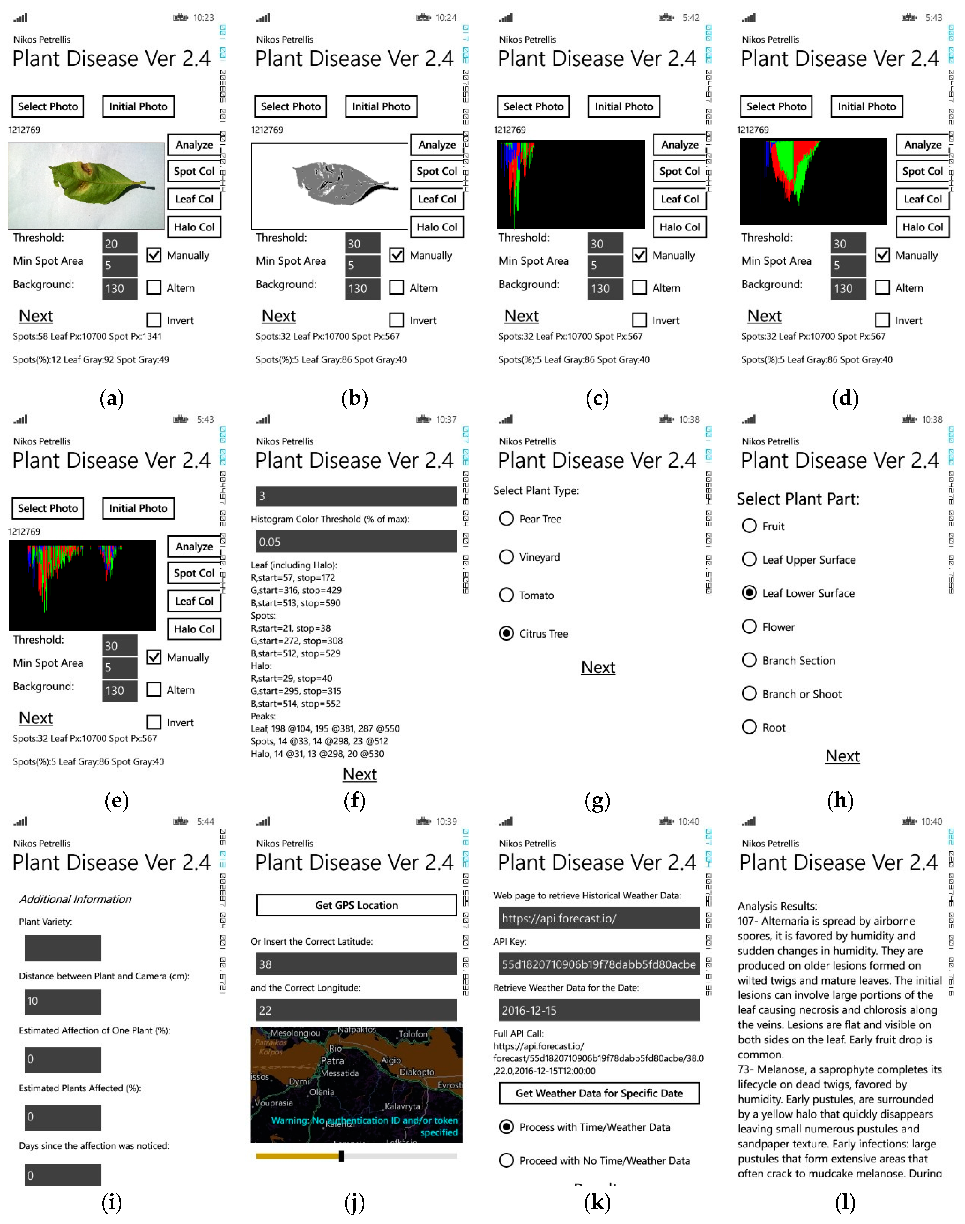
The smart phone application that implements the plant disease method described in the previous section was initially developed for Windows phone platforms and is currently ported to Android and iOS. The basic pages in the Windows phone implementation are shown in Figure 6. In Figure 6a, the main application page is displayed where the user can select a stored photograph of the plant part to be tested. The selection of the appropriate BSM or SSM is performed in this page by altering the corresponding thresholds Bg and Th (SSM1), or by selecting directly SSM2 or SSM3 (through a combination of the “Manual” and “Altern” check boxes). The “Min Spot Area” field defines the minimum number of pixels per spot. Spots that consist of a smaller number of pixels are considered noise and are neglected. The image analysis takes place and an image with four levels of gray appears showing the background in white, the normal leaf (or plant part in general) in gray and the spots in black color (Figure 6b). The halo around the spots is also displayed with white color. The user can interactively switch between the initial color and the resulting gray image to adjust the Bg and Th thresholds for higher segmentation precision. An unsuccessful spot segmentation is not difficult to be recognized even by an inexperienced user as was shown with the examples of Figure 3 and Figure 4.
The draft color histograms of the spots, the normal leaf and the halo can be viewed in real-time as shown in Figure 6c–e, respectively. At the bottom of these pages, estimated features values (e.g., Ns, As, Gs, Gl) are displayed. In administration mode, the page of Figure 6f is displayed with all the histogram features (begin, end, peak). These feature values are required for the definition of new disease signatures. In user mode, all the information displayed in Figure 6c–f can be hidden.
The pages where the plant type and part is selected are shown in Figure 6g,h, respectively. Different disease signatures have to be defined for each (plant type, plant part) pair. In Figure 6i, additional information can be given by the user that could improve the diagnosis accuracy. This information can include the plant variety, draft descriptions about the number of plants and the portion of one plant that has been infected, how long ago the first symptoms noticed, etc. The next application page (Figure 6j) allows the user to select the geolocation of the plant. This is used in order to retrieve publicly available weather metadata for this location from pages like the one offered by OpenWeather [29]. The user can arbitrarily select specific dates in the page shown in Figure 6k. The weather data retrieved for the selected dates are used to estimate the average temperature and moisture features Tn, Tx, Md of Table 1. For example, if three dates are defined by the user, the Tn is the average of the three minimum temperatures measured on these dates. The last page shown in Figure 6l lists the three diseases that achieved the highest score (see Equation (7)) by the plant disease classification method explained in the previous section.
3. Results
In the experimental results presented in this paper, the information set in Figure 6i was not taken into consideration. The classification process did not also take into account the weather data (Tn, Tx, Md) although they are supported by the developed application since the quantitative contribution of these features in the appearance of a disease was difficult to be determined (their weight was set to 0).
Three metrics were measured in order to characterize the quality of the classification procedure: sensitivity, specificity and accuracy. After analyzing all the available photographs, each disease was treated separately and four parameters were estimated: (a) the true positives (TP) were the photographs displaying the specific disease and were recognized correctly, (b) the true negatives (TN) were the photographs that did not display the specific disease and were also recognized correctly, (c) the falsely recognized as negative (FN) and (d) the falsely recognized as positive (FP) to the specific disease. Sensitivity measures how many of the sample photographs displaying the disease have been recognized correctly. Specificity measures how many of the samples that do not display the specific disease, have been recognized correctly. Finally, accuracy indicates how many of both categories have been identified successfully. These metrics are defined as:
The experimental results for each disease of the group A (see Section 2), are presented in Table 2. In each cell, the sensitivity/specificity/accuracy results are displayed. The number of photographs used for training and for testing are listed in parentheses next to the disease name. Similar experimental results for the leaves of group B are presented in Table 3 and the corresponding for the diseases of the orange fruits are listed in Table 4. As can be seen from these tables the number of test photographs per disease ranges between 10 and 56. In most of the diseases, 30–40 photographs were used. Few of them (6–8), were used for training.
The developed application has selected the most likely disease after performing the appropriate analysis. In case of leaves, it had to select between five alternatives while it had to choose the most likely disease between four alternatives in the case of citrus fruits. The columns of the Table 2, Table 3 and Table 4 correspond to the different SSM used. The first column shows the results achieved using SSM1 with an optimal Th value (Th,opt) for accurate image segmentation. The Th,opt value was selected by trial and error. Then, the Th,opt ± 10 values are also tested to examine how worse can the results get if the user does not select the exact Th,opt value but a different one in the range (Th,opt − 10, Th,opt + 10). If the constant 10 is too large to be added to, or subtracted by the threshold, a ±10% is used. The other two columns show the results if the SSM2 and SSM3 are used to segment the input image in a non-interactive way.
The features used by the technique that has been described in Section 2.3 are also tested with popular classification methods in the framework of the Weka tool. The specific classification methods tested are: (a) multilayer perceptron neural network, (b) J48 decision tree [30], (c) random forest [31], (d) random tree (e) naïve Bayes [32] and two more recent approaches that are based on logistic model trees (LMT) and are supported in the Weka environment: (f) simple logistics [33] and (g) LMT [34]. The training and testing of these algorithms is performed using the cross-validation method with the default 10 folders. This means that for each class the test samples are distributed in 10 folders, 9 of them are used for training and the 10th for testing. All the folders are used for testing in a round robin fashion and the classification results obtained are combined. It is obvious that the employed classification methods are trained exhaustively and much more efficiently than the proposed scheme that uses 10–36% of the test samples for training. The sensitivity, specificity and accuracy results of the classification methods tested in Weka are listed in Table 5, Table 6 and Table 7. The sensitivity, specificity and accuracy measured when the photographs of the leaves from both group A (captured under direct sunlight) and group B (captured under a canopy) are merged into a single group (AB), are listed in Table 5. The groups A and B have also been tested separately and the sensitivity, specificity and accuracy results are presented in Table 6 and Table 7.
Color spaces (HSV, HSL, CIE L*a*b) different than RGB have been used with linear DRE (see Equation (3)) for the diagnosis of four pear diseases. An overall set of 200 pear leaf photographs (50 per disease) has been employed and 8 of the 50 photographs from each disease were used for training. The DRE normalization has been applied to the V (value) component of HSV, and the L (lightness) component of HSL or CIE L*a*b. The sensitivity results are listed in Table 8.
4. Discussion
As can be seen from Table 2 and Table 3, higher sensitivity is achieved using the photographs of group A. This is explained by the fact that the plant diseases have been defined based on the photographs from this group. A comparable accuracy is achieved in both groups A and B, since higher sensitivity was achieved in group A, for anthracnose and nutrient deficiency and higher in group B for Alternaria and melanose. Better specificity is achieved in group B. The highest score for these metrics is achieved using SSM1 with optimal Th, although SSM3 is more efficient in some cases. Some performance degradation is expected when a Th value different from the optimal one is used. However, it is not likely that the user would select a threshold Th much different from Th,opt as he/she would be able to compare interactively the initial photograph (Figure 6a) with the segmented one (Figure 6b). Higher accuracy is achieved in group A. In group B the application fails to recognize diseases like anthracnose and nutrient deficiency with acceptable sensitivity since the training photographs of these diseases were not representative of the group B. In group C, the sensitivity achieved is not particularly high for Septoria and fruit split, but the overall accuracy is acceptable in all cases (see Table 4). This is owed mainly to the high specificity that can be achieved in this group. The sensitivity achieved in group C is slightly worse than group A, but much higher than that of group B.
From the comparison with other classification methods presented in Table 5, Table 6 and Table 7 it can be deduced that the highest sensitivity for group A,B is achieved by the proposed method in all diseases but nutrient deficiency. SimpleLogistics is the only compared method that achieves better sensitivity for CCDV (see Table 5). From Table 5 it is also obvious that the proposed method achieves very good accuracy in the case of Alternaria (only random forest is better) and CCDV. However, many of these classification methods achieve higher accuracy than the proposed one in the case of anthracnose, nutrient deficiency and melanose. Focusing on group A, the sensitivity achieved by the proposed method is much better than all the other classification methods except from the case of nutrient deficiency as shown by Table 6. Concerning the results presented in Table 7, the proposed method achieves better sensitivity and accuracy than all the other methods in the case of Alternaria, CCDV and melanose. The accuracy achieved for the other two diseases (anthracnose, nutrient deficiency) is comparable to the accuracy of the rest of the classification methods.
The results achieved by the developed classification technique are generally better in group A and as already mentioned this is owed to the fact that the disease signatures have been defined using photographs from this group. In any case, the accuracy achieved by the proposed method is comparable (if not better) than the rest of the classification algorithms when they operate on the same set of features. It has to be stressed that the results of the compared classification methods are the best that could have been achieved in the Weka tool since cross-validation with 10 folders has been selected. This configuration forces multiple cross checks in order to perform the best possible classification.
The employed normalization technique that has been originally developed for skin disorder diagnosis [35], improved the achieved sensitivity by up to 150% in some cases (e.g., from 45% to 68% in Papillomas). The effect of other normalization techniques such as linear DRE in various color spaces (HSV, HSL, CIE L*a*b) was measured in pear disease diagnosis and the sensitivity results were listed in Table 8. As can be seen from this table, only one of the four diseases achieved better sensitivity in color spaces different than RGB. For this reason, the normalization technique of [35] was employed in the rest of the experiments conducted in the framework of this paper.
The SSM2 and SSM3 achieved worse results compared to the SSM1 with Th,opt. However, it has to be noted that the disease signature definition was based on the analysis performed by SSM1 and Th,opt. Had photographs been analyzed with SSM2 or SSM3 for the disease signature definition, the results would be much better since more representative photographs would have been exploited. Table 9 shows the draft segmentation quality achieved by SSM2 and SSM3. The analysis performed by SSM2 and SSM3 is compared to that of SSM1 with Th,opt. A segmentation precision degradation between 10% and 50% compared to SSM1 is marked as “Moderately Accurate” in Table 9. If the degradation is better, the results are marked as “Accurate”, otherwise as “Inaccurate”. As can be seen from this table, SSM2 achieves better segmentation precision if leaf spots have to be recognized while SSM3 recognizes more accurately the spots on the fruits. This can be explained by the fact that the spots on the fruits have a more distinctive color than the leaf spots. For example, the citrus fruits are yellow while the spots are brown and thus, a clear local minimum appears as required by the SSM3 in order to separate correctly the spots from the normal plant part.
Different plant diseases like the ones that appear on grapevine can be recognized with higher than 88% sensitivity as described in [26] where SSM1 with Th,opt is used. If Th,opt ± 10 is used the sensitivity can fall below 70%. The accuracy achieved with the proposed methods may not be as high as the 98% achieved, for example, by Mohanty et al. [17], but it is comparable to the 91% of the method described by Kulkarni and Patil [18] and to the 93% achieved by the mobile phone application presented in [21]. However, the accuracy presented in these referenced approaches was achieved after training the employed classification methods with thousands of images. Moreover, most of these approaches have not been developed for mobile phones that have limited resources [36].
As a conclusion from the discussion above we can state that the proposed plant disease diagnosis method has achieved very good accuracy compared to standard classification methods and the referenced approaches. The disease signatures defined here, were based on a small number of representative training photographs allowing the extension of the supported set of diseases by an end user that does not have access to the application source code. It is obvious that higher accuracy can be achieved by a larger training set. However, we believe that the size of this training set does not have to be excessively high in order to cover all the possible appearances of a disease with acceptable accuracy. Although the optimal thresholds needed for the image segmentation can be easily selected through the SSM1 interactively, the automatic segmentation performed by SSM2 and SSM3 can also be employed according to the displayed plant part and provided that the employed disease signatures would have been defined using photographs analyzed with these methods.
5. Conclusions
A plant disease recognition method that can support an extensible set of diseases is presented in this paper. This method can be implemented merely by the resources of a smart phone that does not have to be connected to a server. A few photographs of plant parts (e.g., less than 25% of the test set) that have been infected by a disease are used for the extraction of invariant features like the number and area of the spots, color histogram features, weather data, etc. The limits (wide and narrow) of these features are used to define disease signatures employed by a fuzzy clustering method that decides which is the most likely disease displayed in the analyzed photograph. The experimental results show that the disease recognition can be achieved with accuracy between 80% and 98% in most of the cases, competing with several popular classification methods. The achieved accuracy depends on the disease, the number and type of training samples used for the definition of the disease signatures and the employed spot-separation method. The most important advantages of the proposed approach are the extensibility of the supported disease signatures, the low complexity owed to the simple features used for the classification and the independence from the orientation, the resolution and the distance of the camera.
Future work will focus on the support of different plants and diseases. Alternative classification methods like pure fuzzy clustering will also be tested as long as they provide extensibility of the supported set of diseases.
6. Patents
This work is protected by the provisional patents 1009346/13-8-2018 and 1008484/12-5-2015 (Greek Patent Office).
Supplementary Materials
The following are available online at https://www.youtube.com/watch?v=yGRFdQF6pXA, Video S1: Plant Disease ver 2.3 demo.
Author Contributions
N.P.; methodology, software, validation, writing—review and editing.
Funding
This research received no external funding.
Conflicts of Interest
The author declares no conflicts of interest.
References
- Liu, H.; Lee, S.-H.; Chahl, J.-S. A review of recent sensing technologies to detect invertebrates on crops. Precis. Agric. 2017, 18, 635–666. [Google Scholar] [CrossRef]
- Kurtulmus, F.; Lee, W.S.; Vardar, A. Immature peach detection in color images acquired in natural illumination conditions using statistical classifiers and neural network. Precis. Agric. 2014, 15, 57–79. [Google Scholar] [CrossRef]
- Cubero, S.; Lee, W.S.; Aleixos, N.; Albert, F.; Blasco, J. Automated Systems Based on Machine Vision for Inspecting Citrus Fruits from the Field to Postharvest—a Review. Food Bioprocess Technol. 2014, 9, 1623–1639. [Google Scholar] [CrossRef]
- Chaivivatrakul, S.; Dailey, M. Texture-based fruit detection. Precis. Agric. 2014, 15, 662–683. [Google Scholar] [CrossRef]
- Qureshi, W.S.; Payne, A.; Walsh, K.B.; Linker, R.; Cohen, O.; Dailey, M.N. Machine vision for counting fruit on mango tree canopies. Precis. Agric. 2014, 18, 224–244. [Google Scholar] [CrossRef]
- Liu, T.; Wu, W.; Chen, W.; Sun, C.; Zhu, X.; Guo, W. Automated image-processing for counting seedlings in a wheat field. Precis. Agric. 2016, 17, 392–406. [Google Scholar] [CrossRef]
- Behmann, J.; Mahlein, A.K.; Rumpf, T.; Romer, C.; Plumer, L. A review of advanced machine learning methods for the detection of biotic stress in precision crop protection. Precis. Agric. 2015, 16, 239–260. [Google Scholar] [CrossRef]
- Ballesteros, R.; Ortega, J.F.; Hernández, D.; Moreno, M.A. Applications of georeferenced high-resolution images obtained with unmanned aerial vehicles. Part I: Description of image acquisition and processing. Precis. Agric. 2014, 15, 579–592. [Google Scholar] [CrossRef]
- Calderón, R.; Montes-Borrego, M.; Landa, B.B.; Navas-Cortés, J.A.; Zarco-Tejada, P.J. Detection of downy mildew of opium poppy using high-resolution multi-spectral and thermal imagery acquired with an unmanned aerial vehicle. Precis. Agric. 2014, 15, 639–661. [Google Scholar] [CrossRef] [Green Version]
- Petrellis, N. A Review of Image Processing Techniques Common in Human and Plant Disease Diagnosis. Symmetry 2018, 10, 270. [Google Scholar] [CrossRef]
- Deng, X.-L.; Li, Z.; Hong, T.-S. Citrus disease recognition based on weighted scalable vocabulary tree. Precis. Agric. 2014, 16, 321–330. [Google Scholar] [CrossRef]
- Horst, R.K. Westcott’s Plant Disease Handbook, 6th ed.; Kluwer Academic Publishers: Boston, MA, USA, 2001. [Google Scholar]
- Barbedo, G.C.A. Digital image processing techniques for detecting quantifying and classifying plant diseases. Springer Plus 2013, 2, 660. [Google Scholar] [CrossRef]
- Patil, J.; Kumar, R. Advances in image processing for detection of plant diseases. J. Adv. Bioinform. Appl. Res. 2011, 2, 135–141. [Google Scholar]
- Kulkarni, A.; Patil, A. Applying Image Processing Technique to Detect Plant Diseases. Int. J. Mod. Eng. Res. 2012, 2, 3361–3364. [Google Scholar]
- Camargo, A.; Smith, J. Image pattern classification for the identification of disease causing agents in plants. Comput. Electron. Agric. 2009, 66, 121–125. [Google Scholar] [CrossRef]
- Mohanty, S.P.; Hughes, D.P.; Salathé, M. Using Deep Learning for Image-Based Plant Disease Detection. Front. Plant Sci. 2016, 7, 346. [Google Scholar] [CrossRef] [Green Version]
- Lai, J.-C.; Ming, B.; Li, S.-K.; Wang, K.-R.; Xie, R.-Z.; Gao, S.-J. An Image-Based Diagnostic Expert System for Corn Diseases. Agric. Sci. China 2010, 9, 1221–1229. [Google Scholar] [CrossRef]
- Schaad, N.W.; Frederick, R.D. Real-time PCR and its application for rapid plant disease diagnostics. Can. J. Plant Pathol. 2002, 24, 250–258. [Google Scholar] [CrossRef]
- Sankaran, S.; Mishra, A.; Ehsani, R.; Davis, C. A review of advanced techniques for detecting plant diseases. Comput. Electron. Agric. 2010, 72, 1–13. [Google Scholar] [CrossRef]
- Prasad, S.; Peddoju, S.; Ghosh, D. Multi-resolution mobile vision system for plant leaf disease diagnosis. Signal Image Video Process. 2016, 10, 379–388. [Google Scholar] [CrossRef]
- Johannes, A.; Picon, A.; Alvarez-Gila, A.; Echazarra, J.; Rodriguez-Vaamonde, S.; Navajas, A.D.; Ortiz-Barredo, A. Automatic plant disease diagnosis using mobile capture devices, applied on a wheat use case. Comput. Electron. Agric. 2017, 138, 200–209. [Google Scholar] [CrossRef]
- Abu-Naser, S.; Kashkash, K.; Fayyad, M. Developing an Expert System for Plant Disease Diagnosis. J. Artif. Intell. 2008, 1, 78–85. [Google Scholar] [CrossRef]
- Luke, E.; Beckerman, J.; Sadof, C.; Richmond, D.; McClure, D.; Hill, M.; Lu, Y. Purdue Plant Doctor App Suite. Purdue University. Available online: https://www.purdueplantdoctor.com/ (accessed on 16 February 2019).
- Strey, S.; Strey, R.; Burkert, S.; Knake, P.; Raetz, K.; Seyffarth, K.; et al. Plant Doctor app. Available online: https://plantix.net/ (accessed on 16 February 2019).
- Petrellis, N. A Smart Phone Image Processing Application for Plant Disease Diagnosis. In Proceedings of the 2017 6th International Conference on Modern Circuits and Systems Technologies (MOCAST), Thessaloniki, Greece, 4–6 May 2017. [Google Scholar]
- Petrellis, N. Mobile Application for Plant Disease Classification Based on Symptom Signatures. In Proceedings of the 21st Pan-Hellenic Conference on Informatics, Larissa, Greece, 28–30 September 2017; pp. 1–6. [Google Scholar]
- Petrellis, N. Plant Lesion Characterization for Disease Recognition- A windows phone application. In Proceedings of the 2nd International Conference on Frontiers of Signal Processing, Warsaw, Polland, 15–17 October 2016. [Google Scholar]
- OpenWeather. Available online: api.forecast.io (accessed on 16 February 2019).
- Quinlan, R. C4.5: Programs for Machine Learning; Morgan Kaufmann Publishers: San Mateo, CA, USA, 1993. [Google Scholar]
- Breiman, L. Random Forests. Mach. Learn. 2001, 45, 5–32. [Google Scholar] [CrossRef] [Green Version]
- John, G.; Langley, P. Estimating Continuous Distributions in Bayesian Classifiers. In Proceedings of the 11th Conference on Uncertainty in Artificial Intelligence, San Mateo, CA, USA, 18–20 August 1995; pp. 338–345. [Google Scholar]
- Sumner, M.; Frank, E.; Hall, M. Speeding Up Logistic Model Tree Induction. In Lecture Notes in Computer Science; Springe: Berlin, Germany, 2005; pp. 675–683. [Google Scholar]
- Landwehr, N.; Hall, M.; Frank, E. Logistic Model Trees. Mach. Learn. 2005, 95, 161–205. [Google Scholar] [CrossRef]
- Petrellis, Ν. Skin Disorder Diagnosis Assisted by Lesion Color Adaptation. In Proceedings of the 22nd Pan-Hellenic Conference on Informatics, Athens, Greece, 29 November–1 December 2018; pp. 208–212. [Google Scholar]
- Wadhawan, T.; Situ, N.; Lancaster, K.; Yuan, X.; Zouridakis, G. SkinScanc: A Portable Library for Melanoma Detection on Handheld Devices. In Proceedings of the 2011 IEEE International Symposium on Biomedical Imaging: From Nano to Macro, Chicago, IL, USA, 30 March–2 April 2011. [Google Scholar]
Figure 1.
Spot identification method. Separation of the background (a), spot identification (b), initial spot numbering (c) and final spot numbering (d). Notations: BG-background pixel, LF-normal leaf, SP-lesion spot.
Figure 1.
Spot identification method. Separation of the background (a), spot identification (b), initial spot numbering (c) and final spot numbering (d). Notations: BG-background pixel, LF-normal leaf, SP-lesion spot.

Figure 2.
Gray histogram of (a) an image with a citrus leaf infected by the fungus A. citri (Alternaria) or (b) of the citrus leaf only. Gray histogram of (c) an image with a citrus leaf infected by the fungus Diaporthe citri of melanose or (d) of the same citrus leaf only.
Figure 2.
Gray histogram of (a) an image with a citrus leaf infected by the fungus A. citri (Alternaria) or (b) of the citrus leaf only. Gray histogram of (c) an image with a citrus leaf infected by the fungus Diaporthe citri of melanose or (d) of the same citrus leaf only.

Figure 3.
Spot separation for a leaf (upper surface) infected by the fungus Diaporthe citri of melanose. Original image (a), spot separation method (SSM)1 with Th = 20, Bg = 130 (b), SSM1 with Th = 10, Bg = 130 (c), SSM1 with Th = 30, Bg = 130 (d), SSM2 (e), SSM3 (f).
Figure 3.
Spot separation for a leaf (upper surface) infected by the fungus Diaporthe citri of melanose. Original image (a), spot separation method (SSM)1 with Th = 20, Bg = 130 (b), SSM1 with Th = 10, Bg = 130 (c), SSM1 with Th = 30, Bg = 130 (d), SSM2 (e), SSM3 (f).

Figure 4.
Spot separation for a fruit infected by the dematiaceous hyphomycete of Pseudocercospora. Original image (a), SSM1 with Th = 30, Bg = 130 (b), SSM1 with Th = 20, Bg = 130 (c), SSM1 with Th = 40, Bg = 130 (d), SSM2 (e), SSM3 (f).
Figure 4.
Spot separation for a fruit infected by the dematiaceous hyphomycete of Pseudocercospora. Original image (a), SSM1 with Th = 30, Bg = 130 (b), SSM1 with Th = 20, Bg = 130 (c), SSM1 with Th = 40, Bg = 130 (d), SSM2 (e), SSM3 (f).

Figure 5.
Red-green-blue (RGB) color histograms for the leaf (a), the spot (b) and the halo (c) of Figure 3a image. Feature comparison between melanose and Alternaria spots: red (d), green (e) and blue (f) color.
Figure 5.
Red-green-blue (RGB) color histograms for the leaf (a), the spot (b) and the halo (c) of Figure 3a image. Feature comparison between melanose and Alternaria spots: red (d), green (e) and blue (f) color.

Figure 6.
Application pages. The main page before image analysis (a), the main page after image analysis (b), spot histograms (c), leaf histograms (d), halo histograms (e), histogram feature extraction results (f), selection of the plant (g) and the plant part (h), additional information (i), geolocation (j), retrieval of weather data (k) and disease classification results (l).


Table 1.
The features used by the classification process.
| Feature | Notes |
|---|---|
| Number of Spots (Ns) | Spots consisting of less than a predetermined number of pixels can be considered as noise and be ignored |
| Area of the Spots (As) | The ratio of the lesion spot pixels to the ones of the overall plant part |
| Spot grayness (Gs) | The average gray level of the pixels belonging to spots |
| Normal plant part grayness (Gl) | The average gray level of the pixels belonging to the normal plan part |
| Halo grayness (Gh) | The average gray level of the pixels belonging to the halo |
| Average Moisture (Md) | The average daily moisture estimated for a number of dates determined by the user |
| Average Minimum Temperature (Tn) | The average daily minimum temperatures estimated for a number of dates determined by the user |
| Average Maximum Temperature (Tx) | The average daily maximum temperatures estimated for a number of dates determined by the user |
| Beginning of a color histogram (Bcr) | The histogram position of the red (c = R), the rreen (c = G), or the blue (c = B) color of the spot (r = S), the normal plant part (r = L), or the halo (r = H) where the histogram curve crosses upwards the Tbe threshold (9 parameters) |
| Ending of a color histogram (Ecr) | The histogram position of the red (c = R), the green (c = G) or the blue (c = B) color of the spot (r = S), the normal plant part (r = L) or the halo (r = H) where the histogram curve crosses downwards the Tbe threshold (9 parameters) |
| Histogram Peak (Pcr) | The histogram peak position of the red (c = R), the green (c = G) or the blue (c = B) color of the spot (r = S), the normal plant part (r = L) or the Halo (r = H) (9 parameters) |
Table 2.
Sensitivity/specificity/accuracy of group A. The parentheses next to the name of the diseases denote (test/training samples). The SSM with the best accuracy for each disease is highlighted with bold-italics.
Table 2.
Sensitivity/specificity/accuracy of group A. The parentheses next to the name of the diseases denote (test/training samples). The SSM with the best accuracy for each disease is highlighted with bold-italics.
| SSM1 Optimal Th (Th,opt) (%) | SSM1 (Th,opt − 10) (%) | SSM1 (Th,opt + 10) (%) | SSM2 (%) | SSM3 (%) | |
|---|---|---|---|---|---|
| Alternaria (44/6) | 86/78/80 | 82/78/79 | 82/78/79 | 41/96/85 | 63/90/85 |
| Anthracnose (24/6) | 75/92/89 | 73/98/95 | 70/86/84 | 20/84/77 | 89/76/77 |
| CCDV (22/8) | 91/100/99 | 45/100/92 | 91/100/99 | 75/100/98 | 90/99/98 |
| Melanose (36/8) | 86/78/80 | 82/78/79 | 82/78/79 | 41/96/85 | 63/90/85 |
| Nutrient Deficiency (38/8) | 79/96/92 | 74/96/91 | 68/96/89 | 61/94/87 | 18/100/90 |
Table 3.
Sensitivity/specificity/accuracy of group B. The parentheses next to the name of the diseases denote (test/training samples). The SSM with the best accuracy for each disease is highlighted with bold-italics.
Table 3.
Sensitivity/specificity/accuracy of group B. The parentheses next to the name of the diseases denote (test/training samples). The SSM with the best accuracy for each disease is highlighted with bold-italics.
| SSM1 Optimal Th (Th,opt) (%) | SSM1 (Th,opt − 10) (%) | SSM1 (Th,opt + 10) (%) | SSM2 (%) | SSM3 (%) | |
|---|---|---|---|---|---|
| Alternaria (30/6) | 73/94/90 | 60/94/87 | 60/94/87 | 50/95/91 | 70/90/87 |
| Anthracnose (56/6) | 36/87/79 | 31/86/77 | 33/86/78 | 67/79/76 | 71/76/75 |
| CCDV (18/8) | 89/100/99 | 78/100/97 | 78/100/97 | 68/100/98 | 75/100/98 |
| Melanose (36/8) | 94/100/99 | 83/97/94 | 83/97/94 | 80/90/89 | 75/85/84 |
| Nutrient Deficiency (40/8) | 25/100/81 | 25/100/81 | 25/100/81 | 0/99/89 | 25/100/83 |
Table 4.
Sensitivity/specificity/accuracy of group C. The parentheses next to the name of the diseases denote (test/training samples). The SSM with the best accuracy for each disease is highlighted with bold-italics.
Table 4.
Sensitivity/specificity/accuracy of group C. The parentheses next to the name of the diseases denote (test/training samples). The SSM with the best accuracy for each disease is highlighted with bold-italics.
| SSM1 Optimal Th (Th,opt) (%) | SSM1 (Th,opt – 10) (%) | SSM1 (Th,opt + 10) (%) | SSM2 (%) | SSM3 (%) | |
|---|---|---|---|---|---|
| Melanose (26/8) | 100/86/92 | 92/86/88 | 92/86/88 | 92/100/96 | 100/93/96 |
| Rot (20/6) | 80/100/89 | 70/100/89 | 70/100/89 | 80/96/93 | 60/100/86 |
| Septoria (10/6) | 33/100/87 | 20/100/86 | 20/100/86 | 100/100/100 | 20/100/86 |
| Fruit Split (10/6) | 40/100/89 | 40/100/89 | 40/100/89 | 75/100/96 | 40/100/89 |
Table 5.
Sensitivity/specificity/accuracy of the classification methods listed in the 1st column, using the features presented in Table 1 (group AB). The classification method with the best accuracy for each disease is highlighted with bold-italics.
Table 5.
Sensitivity/specificity/accuracy of the classification methods listed in the 1st column, using the features presented in Table 1 (group AB). The classification method with the best accuracy for each disease is highlighted with bold-italics.
| Classification Method | Alternaria (%) | Anthracnose (%) | CCDV (%) | Nutrient Deficiency (%) | Melanose (%) |
|---|---|---|---|---|---|
| Multilayer Perceptron | 37/84/86 | 33/89/90 | 82/97/97 | 85/92/96 | 56/87/91 |
| J48 | 44/80/87 | 14/88/87 | 64/95/94 | 79/93/95 | 56/86/91 |
| Random Forest | 59/88/91 | 14/93/87 | 73/97/95 | 91/90/98 | 44/89/89 |
| Random Tree | 34/79/85 | 14/84/87 | 73/94/95 | 68/92/92 | 37/83/87 |
| Naïve Bayes | 6/99/78 | 19/91/87 | 59/96/93 | 91/88/98 | 67/63/93 |
| Simple Logistics | 34/86/85 | 14/89/87 | 91/96/97 | 91/93/98 | 70/88/94 |
| LMT | 34/85/85 | 19/86/87 | 82/96/97 | 88/92/97 | 59/89/92 |
| Proposed | 82/90/87 | 52/79/73 | 87/100/97 | 50/100/80 | 96/82/85 |
Table 6.
Sensitivity/specificity/accuracy of the classification methods listed in the 1st column, using the features presented in Table 1 (group A). The classification method with the best accuracy for each disease is highlighted with bold-italics.
Table 6.
Sensitivity/specificity/accuracy of the classification methods listed in the 1st column, using the features presented in Table 1 (group A). The classification method with the best accuracy for each disease is highlighted with bold-italics.
| Classification Method | Alternaria (%) | Anthracnose (%) | CCDV (%) | Nutrient Deficiency (%) | Melanose (%) |
|---|---|---|---|---|---|
| Multilayer Perceptron | 39/80/83 | 17/85/85 | 83/94/97 | 93/92/98 | 30/89/89 |
| J48 | 33/75/82 | 25/82/86 | 58/93/92 | 73/96/94 | 50/88/91 |
| Random Forest | 50/75/86 | 33/89/88 | 75/96/95 | 87/90/97 | 40/95/91 |
| Random Tree | 39/69/84 | 33/89/86 | 58/94/92 | 73/94/94 | 30/86/89 |
| Naïve Bayes | 11/92/76 | 25/89/86 | 75/94/95 | 93/92/98 | 50/70/92 |
| Simple Logistics | 44/90/85 | 50/87/91 | 83/91/97 | 80/88/95 | 40/93/91 |
| LMT | 44/90/85 | 50/87/91 | 83/93/97 | 87/88/97 | 40/93/91 |
| Proposed | 86/78/80 | 75/92/89 | 91/100/99 | 79/96/92 | 90/92/92 |
Table 7.
Sensitivity/specificity/accuracy of the classification methods listed in the 1st column, using the features presented in Table 1 (group B). The classification method with the best accuracy for each disease is highlighted with bold-italics.
Table 7.
Sensitivity/specificity/accuracy of the classification methods listed in the 1st column, using the features presented in Table 1 (group B). The classification method with the best accuracy for each disease is highlighted with bold-italics.
| Classification Method | Alternaria (%) | Anthracnose (%) | CCDV (%) | Nutrient Deficiency (%) | Melanose (%) |
|---|---|---|---|---|---|
| Multilayer Perceptron | 50/91/90 | 45/86/91 | 70/97/96 | 84/90/96 | 50/87/88 |
| J48 | 36 | 0/93/84 | 50/93/93 | 58/80/88 | 31/81/84 |
| Random Forest | 29/87/86 | 18/91/87 | 70/95/96 | 79/88/94 | 62/80/91 |
| Random Tree | 36/87/87 | 45/88/91 | 70/93/96 | 74/90/93 | 44/83/87 |
| Naïve Bayes | 7/89/81 | 54/86/93 | 50/90/93 | 68/88/91 | 44/78/87 |
| Simple Logistics | 50/87/90 | 27/86/88 | 70/97/96 | 84/90/96 | 50/87/88 |
| LMT | 43/86/88 | 27/86/88 | 60/97/94 | 84/84/96 | 37/87/86 |
| Proposed | 73/94/91 | 36/87/80 | 89/100/98 | 25/100/81 | 94/100/98 |
Table 8.
Sensitivity of pear disease diagnosis when linear dynamic range expansion (DRE) normalization is employed. The color space with the best sensitivity for each disease is highlighted with bold-italics.
Table 8.
Sensitivity of pear disease diagnosis when linear dynamic range expansion (DRE) normalization is employed. The color space with the best sensitivity for each disease is highlighted with bold-italics.
| Classification Method | RGB | HSV | HSL | CIE L*a*b |
|---|---|---|---|---|
| Fire Blight | 95.8% | 79.2% | 83.3% | 83.3% |
| Pear Scab | 74% | 98% | 98% | 91.6% |
| Mycosphaerella | 100% | 96% | 94% | 90% |
| Mildew | 100% | 88% | 100% | 98% |
Table 9.
Segmentation quality of spot separation method (SSM)2/SSM3.
| SSM | Group | Inaccurate | Moderately Accurate | Accurate |
|---|---|---|---|---|
| SSM2 | A (Direct Sunlight) | 1% | 36% | 63% |
| B (Canopy) | 2% | 35% | 63% | |
| C (Fruit) | 0% | 75% | 25% | |
| SSM3 | A (Direct Sunlight) | 19% | 44% | 37% |
| B (Canopy) | 23% | 49% | 28% | |
| C (Fruit) | 0% | 42% | 58% |
© 2019 by the author. Licensee MDPI, Basel, Switzerland. This article is an open access article distributed under the terms and conditions of the Creative Commons Attribution (CC BY) license (http://creativecommons.org/licenses/by/4.0/).
Share and Cite
MDPI and ACS Style
Petrellis, N. Plant Disease Diagnosis for Smart Phone Applications with Extensible Set of Diseases. Appl. Sci. 2019, 9, 1952. https://0-doi-org.brum.beds.ac.uk/10.3390/app9091952
AMA Style
Petrellis N. Plant Disease Diagnosis for Smart Phone Applications with Extensible Set of Diseases. Applied Sciences. 2019; 9(9):1952. https://0-doi-org.brum.beds.ac.uk/10.3390/app9091952
Chicago/Turabian StylePetrellis, Nikos. 2019. "Plant Disease Diagnosis for Smart Phone Applications with Extensible Set of Diseases" Applied Sciences 9, no. 9: 1952. https://0-doi-org.brum.beds.ac.uk/10.3390/app9091952
Note that from the first issue of 2016, this journal uses article numbers instead of page numbers. See further details here.