Differences in Performance of Models for Heterogeneous Cores during Pulse Decay Tests

Featured Application

Evaluate the permeability of unconventional reservoir cores.

Abstract

Shale and fractured cores often exhibit dual-continuum medium characteristics in pulse decay testing. Dual-continuum medium models can be composed of different flow paths, interporosity flow patterns, and matrix shapes. Various dual-continuum medium models have been used by researchers to analyze the results of pulse decay tests. But the differences in their performance for pulse decay tests have not been comprehensively investigated. The characteristics of the dual-permeability model and the dual-porosity model, the slab matrix, and the spherical matrix in pulse decay testing are compared by numerical modeling in this study. The pressure and pressure derivative curves for different vessel volumes, storativity ratios, interporosity flow coefficients, and matrix-fracture permeability ratios were compared and analyzed. The study found that these models have only a small difference in the interporosity flow stage, and the difference in the matrix shape is not important, and the matrix shape cannot be identified by pulse decay tests. When the permeability of the low permeability medium is less than 1% of the permeability of the high permeability medium, the difference between the dual-permeability model and the dual-porosity model can be ignored. The dual-permeability model approaches the pseudo-steady-state model as the interporosity flow coefficient and vessel volume increase. Compared with the dual-porosity model, the dual-permeability model has a shorter horizontal section of the pressure derivative in the interporosity flow stage. Finally, the conclusions were verified against a case study. This study advances the ability of pulse decay tests to investigate the properties of unconventional reservoir cores.

1. Introduction

In the past two decades, the development of unconventional oil and gas, such as tight sandstone oil and gas, shale gas, and coalbed methane, has received great attention and made has achieved major breakthroughs. Unconventional reservoirs often develop pores and fractures at different scales, showing heterogeneity at the core scale. Its matrix is tight, and its permeability is very low. A key factor limiting the development of unconventional oil and gas is the evaluation of reservoir permeability. One method is to obtain reservoir permeability through well testing and rate transient analysis [1,2,3]. This method needs to solve the unsteady flow of wells under constant bottom hole pressure or constant production rate conditions. The tight formation exhibited non-Darcy flow characteristics, and the solution of its pressure transient is a difficult problem. Dejam et al. [4] obtained the analytical solution of the pressure transient of radial non-Darcy flow by the generalized Boltzmann transformation method. Another method is to perform laboratory core permeability testing. The permeability of tight rock cores is very low, and it takes a very long time to test its permeability by the steady-state method. Given this situation, Brace et al. [5] proposed a pulse decay test method. The apparatus for the method consists of an upstream and downstream vessel and a core holder (Figure 1). By applying a pressure pulse, a pressure difference is created between the upstream and downstream vessels to drive the fluid through the core, causing the pressure of the upstream and downstream vessels to decrease or recover. Then, the permeability of the core can be obtained by analyzing the pressure data over time [6,7]. Due to the good adaptability of the pulse decay test method to low permeability cores, it is widely used in the permeability testing of tight cores, such as tight sandstone, coal rock, and shale [8,9,10,11].

The analysis method for the pulse decay test originally proposed by Brace ignores the pore volume compressibility, which will affect the accuracy of the analysis results. Later, Hsieh et al. [6] proposed a general analytical solution. Based on this solution, Dicker and Smits [12] and Jones [7] simplified this analytical solution and obtained practical analysis methods. Cui et al. [13] extended the analytical solution to consider gas adsorption by modifying the porosity. However, these analytical solutions are based on the Darcy flow of a slightly compressible fluid in a homogenous core. The pressure pulse is generally small, and this condition can be approximately satisfied, whereby the apparent permeability can be obtained. Numerical modeling studies have shown that when the pressure pulse is large, the gas compressibility [14,15], slippage effect, and stress sensitivity [16] will affect the test results. At this time, the analytical methods cannot be applied, and the numerical modeling for historical fitting becomes the basic means.

Heterogeneous cores can often be encountered in tests. They contain fractures or alternating layers of different permeability, especially shale. The phenomenon of backflow in pressure history is considered a dual-continuum medium feature [17,18,19]. In the early 1990s, Kamath et al. [20] and Ning et al. [21] simulated a pulse decay test for cores with a single fracture and proposed a simplified analytical model. Cronin et al. [22,23] carried out pulse decay testing on shale cores with alternating layers of high and low permeability and used a dual-permeability model to analyze the test data. Liu et al. [24] studied the late-time behavior of pulse decay tests for dual-porosity cores and proposed a simplified analytical model. Jia et al. [25,26] simulated the effects of the fracture and vug on pulse decay tests. Alnoaimi and Kovscek [27] fitted a shale pulse decay test with microcracks by numerical modeling and analyzed the effects of the microcrack on shale permeability and storage capacities. Bajaalah [28] studied the pulse decay test for a dual-porosity core with fluid flowing along the radial plane of the cylindrical core, which is different from the conventional axial flow. Han et al. [29] systematically simulated pulse decay tests for a dual-porosity model and proposed a pressure derivative method to analyze the data, which can diagnose whether the cores conform to dual-porosity models through early time pressure data and interporosity flow models by transition stage data.

However, a variety of models have been proposed to characterize dual-continuum media. According to the flow pathway of the system, they can be divided into the dual-porosity models and dual-permeability models. The dual-porosity model can be divided into a pseudo-steady-state model and a transient model based on the interporosity flow patterns. In practice, the shape of the matrix varies widely, but the models assume several typical shapes, such as slab, sphere, and cylinder. For pulse decay tests, different models will exhibit different characteristics. But the pressure curves of pulse decay tests for different dual-continuum medium models are very similar. The differences in performance of different models in the pulse decay testing, and which model is more suitable for a specific core is still unclear.

In this paper, the pressure and pressure derivative curves of the pulse decay test for dual-permeability and dual-porosity models, sphere matrix, and slab matrix are investigated by numerical modeling. The characteristics of different models in the pulse decay test are clarified and verified by examples.

2. Dual-Continuum Medium Models

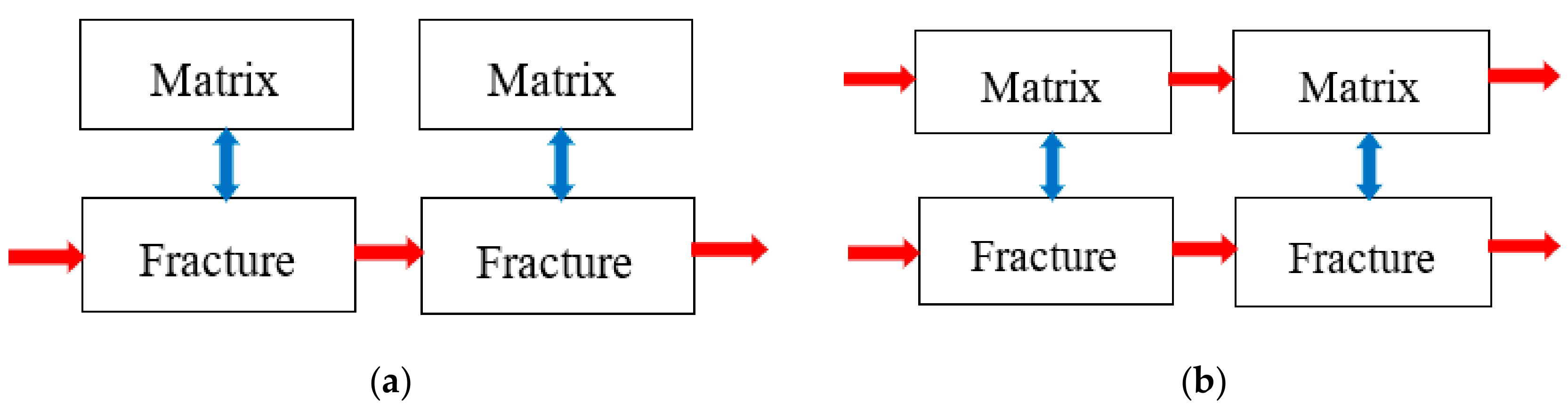
When the RVE (representative elementary volume) of the core is composed of two media with very different permeability, it can be characterized by a dual-continuum medium model. Generally, the higher permeability medium is fractures, and the lower permeability medium is matrixes. Some cores exhibit alternating layers of high and low permeability. For the sake of convenience, all higher permeability media are uniformly called the fractures, and all lower permeability media are uniformly called the matrixes. If the fracture constitutes only the flow pathway of the RVE system, and interporosity flow happens between the matrix and the fracture, the core can be characterized by a dual-porosity model. When both the fracture and the matrix constitute the flow pathway of the REV system, and there is fluid exchange between the fracture and the matrix, it can be characterized by a dual-permeability model. The flow characteristics of different models are shown in Figure 2.

For the shape of the matrix, the aspect ratio of the slab and the sphere is at the two extremes, representing the flow direction between the matrix and the fracture from one dimension to three dimensions. Therefore, only these two matrix shapes will be discussed.

For the pulse decay test, the following assumptions can be made: (1) The temperature is constant during the testing; (2) the test uses a single-phase fluid that is slightly compressible with a constant compressibility; (3) changes in the permeability, pore compressibility, and fluid viscosity with pressure are ignored; (4) the flow in the sample follows Darcy’s law, and the quadratic pressure gradient term can be ignored; and (5) gas leakage is negligible, and the upstream and downstream vessels can be regarded as isobaric bodies.

Based on these assumptions, the mathematical models for the pulse decay test can be established. Han et al. [29] discussed in detail the pulse decay test of the pseudo-steady-state dual-porosity model and transient dual-permeability model with a slab matrix, and the corresponding models and numerical solution methods are given in detail. Therefore, they will not be described here. For the dual-porosity model with a sphere matrix and the dual-permeability model, their mathematical equations and numerical solution method are detailed in Appendix A and Appendix B, respectively. All dimensionless parameters, such as t_D, p_D, the storativity ratio, and the interporosity flow coefficient, are defined in Appendix A. The dimensionless pressure derivative p′_D is defined as the derivative of the dimensionless pressure p_D with respect to the dimensionless time t_D. Various dimensionless dual-continuum medium models are shown in

Table 1. Comparison of dimensionless dual-continuum medium models.

	Dual-Porosity Model		Dual-Permeability Model
	Pseudo-Steady State	Transient
Governing equation	$\begin{array}{l}\omega \frac{\partial p_{\mathrm{fD}}}{\partial t_{\mathrm{D}}}=\frac{\partial p_{\mathrm{fD}}^2}{\partial x_{\mathrm{D}}^2}\\ +{\lambda }_{\mathrm{D}}\left(p_{\mathrm{mD}}-p_{\mathrm{fD}}\right)\end{array}$	$\omega \frac{\partial p_{\mathrm{fD}}}{\partial t_{\mathrm{D}}}=\frac{\partial }{\partial x_{\mathrm{D}}}\left(\frac{\partial p_{\mathrm{fD}}}{\partial x_{\mathrm{D}}}\right)+{\left.\frac{{\lambda }_{\mathrm{D}}}{6}\frac{\partial p_{\mathrm{mD}}}{\partial z_{\mathrm{D}}}\right|}_{z_{\mathrm{D}}=0}$ (slab)	$\omega \frac{\partial p_{\mathrm{fD}}}{\partial t_{\mathrm{D}}}=\frac{{\partial }^2{p}_{\mathrm{fD}}}{\partial x_{\mathrm{D}}^2}+{\lambda }_{\mathrm{D}}\left(p_{\mathrm{mD}}-p_{\mathrm{fD}}\right)$
		$\omega \frac{\partial p_{\mathrm{fD}}}{\partial t_{\mathrm{D}}}=\frac{\partial }{\partial x_{\mathrm{D}}}\left(\frac{\partial p_{\mathrm{fD}}}{\partial x_{\mathrm{D}}}\right)-{\left.\frac{{\lambda }_{\mathrm{D}}}{5}\frac{\partial p_{\mathrm{mD}}}{\partial r_{\mathrm{D}}}\right|}_{r_{\mathrm{D}}=1}$(sphere)
	$\begin{array}{l}-{\lambda }_{\mathrm{D}}\left(p_{\mathrm{mD}}-p_{\mathrm{fD}}\right)\\ =\left(1-\omega \right)\frac{\partial p_{\mathrm{mD}}}{\partial t_{\mathrm{D}}}\end{array}$	$\frac{12\left(1-\omega \right)}{{\lambda }_{\mathrm{D}}}\frac{\partial p_{\mathrm{mD}}}{\partial t_{\mathrm{D}}}=\frac{{\partial }^2{p}_{\mathrm{mD}}}{\partial z_{\mathrm{D}}^2}$(slab)	$\begin{array}{l}\left(1-\omega \right)\frac{\partial p_{\mathrm{mD}}}{\partial t_{\mathrm{D}}}=\frac{k_{\mathrm{m}}}{k_{\mathrm{f}}}\frac{{\partial }^2{p}_{\mathrm{mD}}}{\partial x_{\mathrm{D}}^2}\\ -{\lambda }_{\mathrm{D}}\left(p_{\mathrm{mD}}-p_{\mathrm{fD}}\right)\end{array}$
		$\frac{15\left(1-\omega \right)}{{\lambda }_{\mathrm{D}}}\frac{\partial p_{\mathrm{mD}}}{\partial t_{\mathrm{D}}}=\frac{1}{r_{\mathrm{D}}^2}\frac{\partial }{\partial r_{\mathrm{D}}}\left(r_{\mathrm{D}}^2\frac{\partial p_{\mathrm{mD}}}{\partial r_{\mathrm{D}}}\right)$(sphere)
Initial condition	$$\begin{gathered} \begin{array}{l}{p}_{\mathrm{fD}}\left(x_{\mathrm{D}},0\right)=p_{\mathrm{mD}}\left(x_{\mathrm{D}},0\right)\\ =0 \\ 0<x_{\mathrm{D}}<1\end{array} \end{gathered}$$	$\begin{array}{l}{p}_{\mathrm{fD}}\left(x_{\mathrm{D}},0\right)=p_{\mathrm{mD}}\left(x_{\mathrm{D}},z_{\mathrm{D}},0\right)=0\\ 0\le z_{\mathrm{D}}\le 1/2,0<x_{\mathrm{D}}<1\end{array}$ (slab) $\begin{array}{l}{p}_{\mathrm{fD}}\left(x_{\mathrm{D}},0\right)=p_{\mathrm{mD}}\left(x_{\mathrm{D}},r_{\mathrm{D}},0\right)=0\\ 0<x_{\mathrm{D}}<1\end{array}$ (sphere)	$\begin{array}{l}{p}_{\mathrm{fD}}\left(x_{\mathrm{D}},0\right)=p_{\mathrm{mD}}\left(x_{\mathrm{D}},0\right)=0,\\ 0<x_{\mathrm{D}}<1\end{array}$
	$p_{\mathrm{fD}}\left(0,0\right)=p_{\mathrm{uD}}\left(0\right)=1$	$p_{\mathrm{fD}}\left(0,0\right)=p_{\mathrm{uD}}\left(0\right)=1$	$p_{\mathrm{fD}}\left(0,0\right)=p_{\mathrm{uD}}\left(0\right)=1$
	$p_{\mathrm{fD}}\left(1,0\right)=p_{\mathrm{dD}}\left(0\right)=0$	$p_{\mathrm{fD}}\left(1,0\right)=p_{\mathrm{dD}}\left(0\right)=0$	$p_{\mathrm{fD}}\left(1,0\right)=p_{\mathrm{dD}}\left(0\right)=0$
Boundary conditions	$\begin{array}{l}{p}_{\mathrm{fD}}\left(0,t_{\mathrm{D}}\right)=p_{\mathrm{uD}}\left(t_{\mathrm{D}}\right)\\ t_{\mathrm{D}}>0\end{array}$	$p_{\mathrm{fD}}\left(0,t_{\mathrm{D}}\right)=p_{\mathrm{uD}}\left(t_{\mathrm{D}}\right),t_{\mathrm{D}}>0$	$\begin{array}{l}{p}_{\mathrm{fD}}\left(0,t_{\mathrm{D}}\right)=p_{\mathrm{mD}}\left(0,t_{\mathrm{D}}\right)\\ =p_{\mathrm{uD}}\left(t_{\mathrm{D}}\right),t_{\mathrm{D}}>0\end{array}$
	$\begin{array}{l}{p}_{\mathrm{fD}}\left(1,t_{\mathrm{D}}\right)=p_{\mathrm{dD}}\left(t_{\mathrm{D}}\right)\\ t_{\mathrm{D}}>0\end{array}$	$p_{\mathrm{fD}}\left(1,t_{\mathrm{D}}\right)=p_{\mathrm{dD}}\left(t_{\mathrm{D}}\right),t_{\mathrm{D}}>0$	$\begin{array}{l}{p}_{\mathrm{fD}}\left(1,t_{\mathrm{D}}\right)=p_{\mathrm{mD}}\left(1,t_{\mathrm{D}}\right)\\ =p_{\mathrm{dD}}\left(t_{\mathrm{D}}\right),t_{\mathrm{D}}>0\end{array}$
	$\begin{array}{l}\frac{d{p}_{\mathrm{uD}}}{d{t}_{\mathrm{D}}}=A_{\mathrm{u}}{\left.\frac{\partial p_{\mathrm{fD}}}{\partial x_{\mathrm{D}}}\right|}_{x_{\mathrm{D}}=0}\\ t_{\mathrm{D}}>0\end{array}$	$\frac{d{p}_{\mathrm{uD}}}{d{t}_{\mathrm{D}}}=A_{\mathrm{u}}{\left.\frac{\partial p_{\mathrm{fD}}}{\partial x_{\mathrm{D}}}\right|}_{x_{\mathrm{D}}=0},t_{\mathrm{D}}>0$	$\begin{array}{l}\frac{d{p}_{\mathrm{uD}}}{d{t}_{\mathrm{D}}}=A_{\mathrm{u}}{\left.\frac{\partial p_{\mathrm{fD}}}{\partial x_{\mathrm{D}}}\right|}_{x_{\mathrm{D}}=0}\\ +A_{\mathrm{u}}{\left.\frac{k_{\mathrm{m}}}{k_{\mathrm{f}}}\frac{\partial p_{\mathrm{mD}}}{\partial x_{\mathrm{D}}}\right|}_{x_{\mathrm{D}}=0},t_{\mathrm{D}}>0\end{array}$
	$\begin{array}{l}\frac{d{p}_{\mathrm{dD}}}{d{t}_{\mathrm{D}}}=-A_{\mathrm{d}}{\left.\frac{\partial p_{\mathrm{fD}}}{\partial x_{\mathrm{D}}}\right|}_{x_{\mathrm{D}}=1}\\ t_{\mathrm{D}}>0\end{array}$	$\frac{d{p}_{\mathrm{dD}}}{d{t}_{\mathrm{D}}}=-A_{\mathrm{d}}{\left.\frac{\partial p_{\mathrm{fD}}}{\partial x_{\mathrm{D}}}\right|}_{x_{\mathrm{D}}=1},t_{\mathrm{D}}>0$	$\begin{array}{l}\frac{d{p}_{\mathrm{dD}}}{d{t}_{\mathrm{D}}}=-A_{\mathrm{d}}{\left.\frac{\partial p_{\mathrm{fD}}}{\partial x_{\mathrm{D}}}\right|}_{x_{\mathrm{D}}=1}\\ -A_{\mathrm{d}}{\left.\frac{k_{\mathrm{m}}}{k_{\mathrm{f}}}\frac{\partial p_{\mathrm{mD}}}{\partial x_{\mathrm{D}}}\right|}_{x_{\mathrm{D}}=1},t_{\mathrm{D}}>0\end{array}$
		${\left.\frac{\partial p_{\mathrm{mD}}}{\partial z_{\mathrm{D}}}\right|}_{z_{\mathrm{D}}=1/2}=0$,${\left.p_{\mathrm{mD}}\right|}_{z_{\mathrm{D}}=0}=p_{\mathrm{fD}}$ (slab) ${\left.\frac{\partial p_{\mathrm{m}}}{\partial r_{\mathrm{D}}}\right|}_{r_{\mathrm{D}}=0}=0$,${\left.p_{\mathrm{mD}}\right|}_{r_{\mathrm{D}}=1}=p_{\mathrm{fD}}$(sphere)

. The dimensionless models show that the models are determined by the ratio of pore-vessel storativity (for simplicity in the following, only the vessel volume is discussed), the storativity ratio, the interporosity flow coefficient, and the matrix-fracture permeability ratio. The proposed numerical method is used to simulate the pulse decay test of the dual-continuum medium models in the following.

3. Dual-Porosity Model with Different Matrix Shape

3.1. Effect of Vessel Volume

Figure 3 shows the numerical modeling results of pulse decay tests for the dual-porosity core under different vessel volumes. It should be noted that all parameters as axes in the following figures are dimensionless, and only the pressure and pressure derivative for upstream and downstream vessels are presented in these figures. Although the dimensionless pressure derivatives presented in the figure are as small as 10⁻⁹, their dimensional values may be considerable. In the early stages (for A_d = A_u = 10, t_D < 1) and the equilibrium stages (for A_d = A_u = 10, t_D > 10⁴), the pressure and pressure derivatives of the two are completely coincident. Only during the interporosity flow stages (for A_d = A_u = 10, 10 < t_D < 10⁴), is there a difference. As the vessel volume increases (i.e., A_u decrease), the difference in the pressure and pressure derivative curves of the sphere and slab matrix continually decrease, and the characteristics of the dual-porosity medium become weaker. When 0.1 < A_u = A_d < 10 (the range suggested by Han et al. [29]), although there are some differences between the sphere and slab matrix, it is very small. In the following figures, double logarithmic coordinates are used for curves of pressure derivatives so that the shape of the plots does not change due to differences in dimensions. Pressure derivative curves of different dimensions can be completely coincident by translation.

3.2. Effect of Storativity Ratio

The numerical modeling results of pulse decay tests for the dual-porosity medium at different storativity ratios are shown in Figure 4. The pressure and pressure derivative curves of both the early (t_D < 10) and equilibrium stages (t_D > 10⁵) are completely coincident, and only slightly different in the interporosity flow stage (10 < t_D < 10⁵). The pressure in the interporosity flow stage decreases as the storativity ratio increases, but the pressure derivative is less affected by it. As the storativity ratio increases, the pressure derivative decreases slightly. The difference in pressure derivatives of different matrix shapes during the interporosity flow stage is almost unaffected by the storativity ratio.

3.3. Effect of Interporosity Flow Coefficient

The numerical modeling results of pulse decay tests for dual-porosity cores with different interporosity flow coefficients are shown in Figure 5. At the early stage (t_D < 1) and the equilibrium stage (for λ = 10⁻⁴, t_D > 10⁵), the pressure and pressure derivative curves of the sphere and slab matrix coincide, except for a slight difference in the interporosity flow stage (for λ = 10⁻⁴, 1 < t_D < 10⁵). The pressure derivatives of the two in the interporosity flow stage are close in shape and value and cannot be distinguished. At the same time, the interporosity flow coefficient has little effect on the difference between the two.

4. Comparison of Dual-Porosity and Dual-Permeability Models

4.1. Effect of Vessel Volume

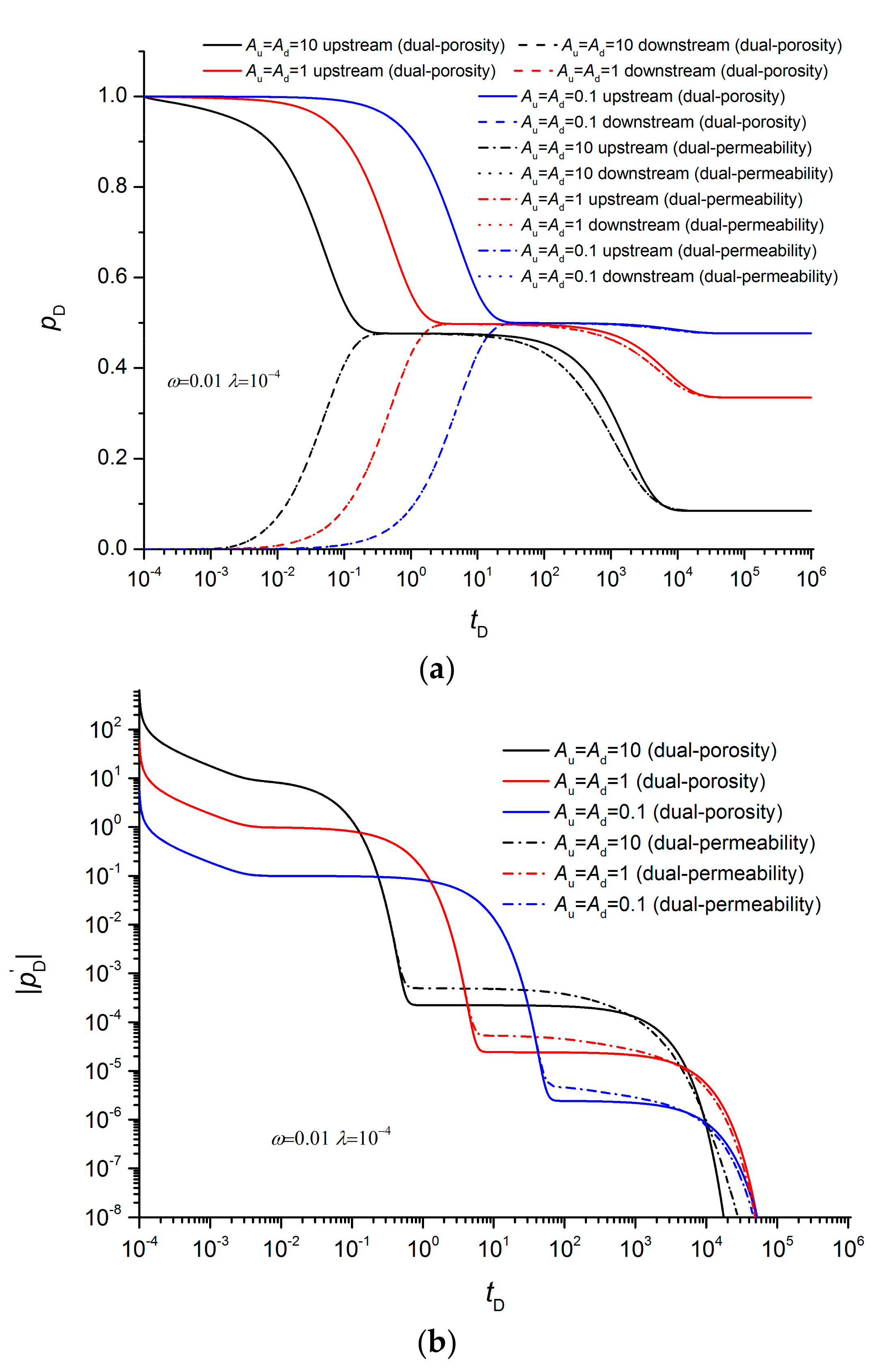
The effect of different vessel volumes on pulse decay tests for the dual-permeability and dual-porosity cores is shown in Figure 6. Since the interporosity flow model between the matrix and the fracture of the dual-permeability model belongs to the pseudo-steady-state, it is later compared with the pseudo-steady-state dual-porosity model. In the early (for A_u = A_d = 1, t_D < 10) and equilibrium (for A_u = A_d = 1, t_D > 10⁵) stages, the pressure and pressure derivative of the dual-permeability and dual-porosity cores coincide. Only in the interporosity flow (for A_u = A_d = 1, 10 < t_D < 10⁵) stage, is there a difference. The flow of the dual-permeability model is slightly faster than the flow of the dual-porosity model. As the vessel volume decreases, the difference in the pressure curve of the dual-permeability core and the dual-porosity core is more marked. The difference in the pressure derivative is not affected by the vessel volume. The pressure derivatives of the two are slightly different in the interporosity flow stage, but their shapes are similar. The horizontal section of the pressure derivative curve of the dual-permeability core is relatively short, and the descending speed after the horizontal section is relatively slow. When the pore volume is small, or the vessel is large, the shape of the pressure derivative curve approaches the shape of the transient interporosity flow model.

4.2. Effect of Storativity Ratio

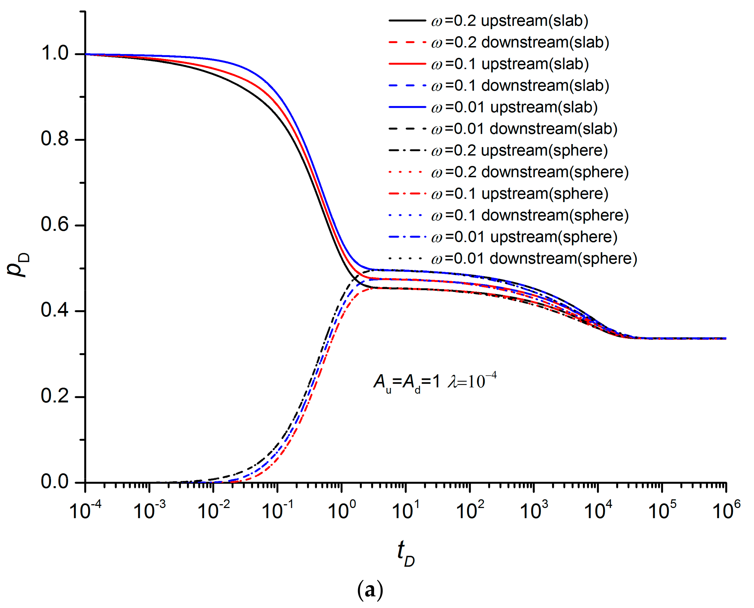
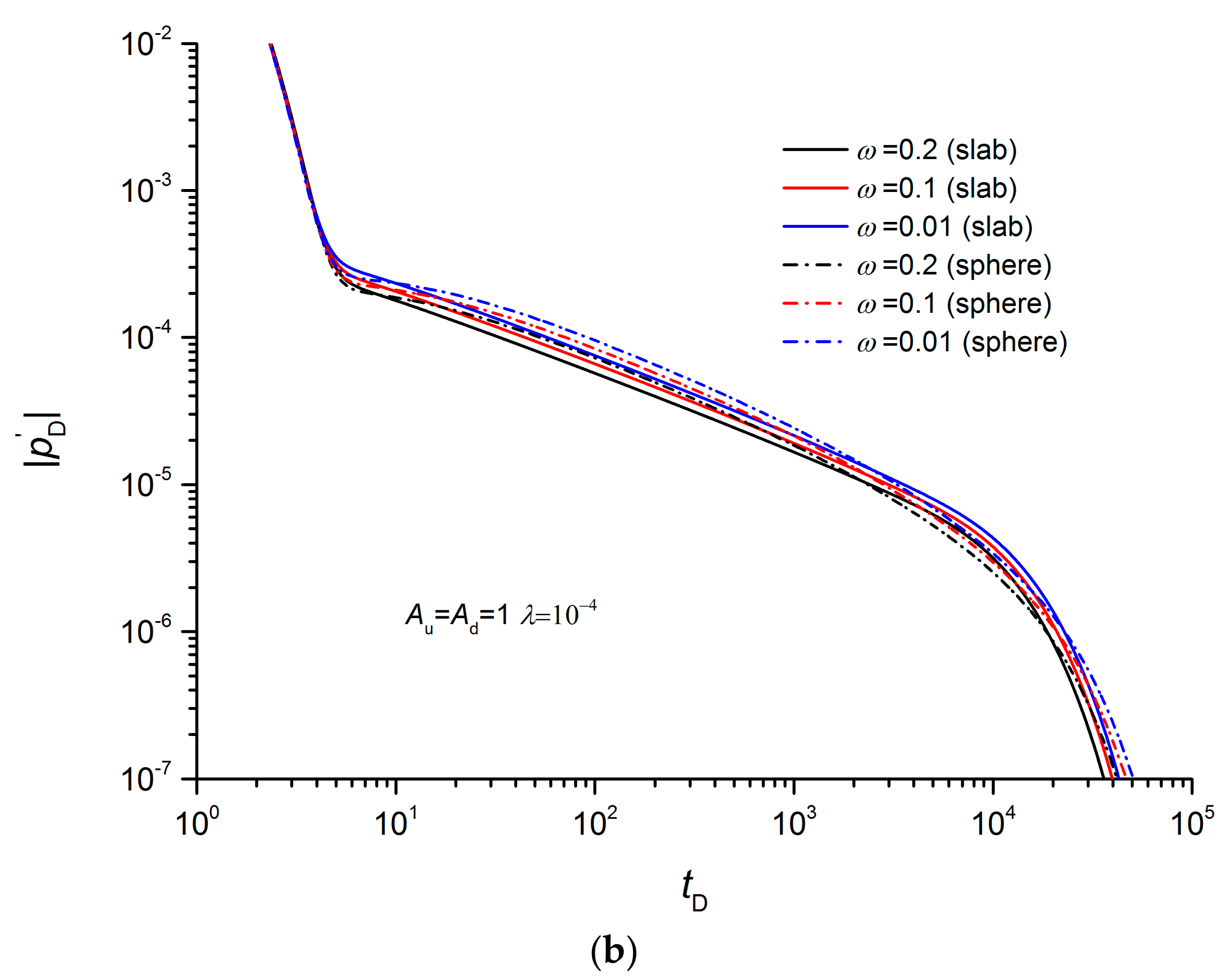
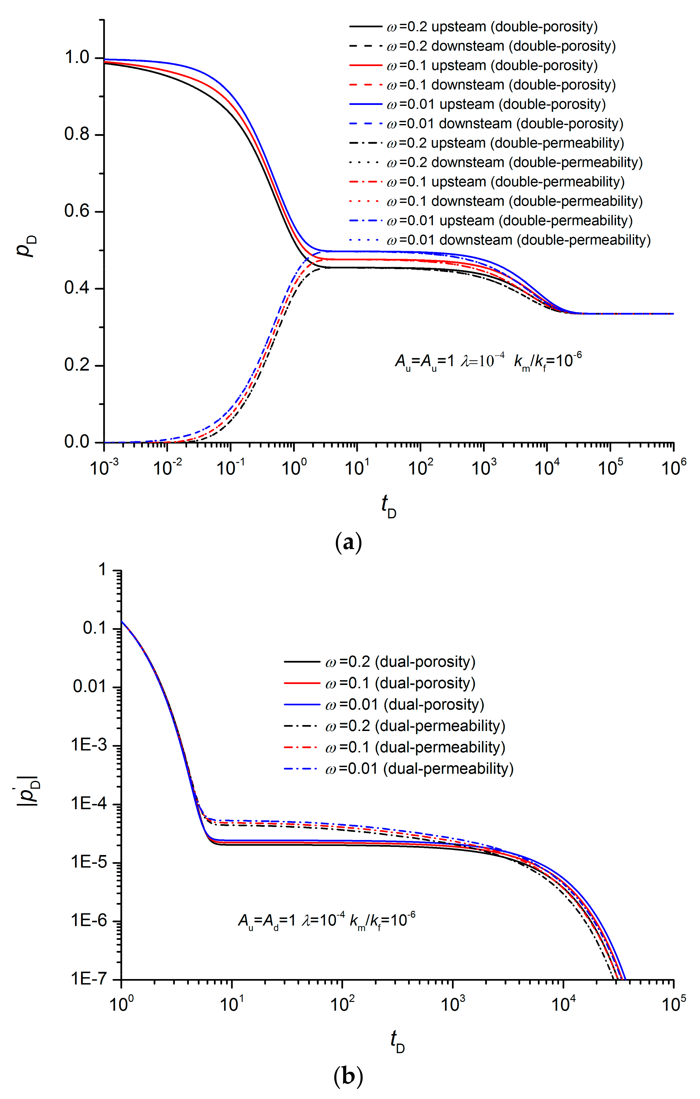
The numerical modeling results of pulse decay tests for dual-permeability and dual-porosity cores with different storativity ratios are shown in Figure 7. In the early (t_D < 10) and equilibrium (t_D > 10⁵) stages, the pressure and pressure derivatives of the two coincide, and are only slightly different during the interporosity flow (10 < t_D < 10⁵) stage. The effect of storativity ratios on the velocity of interporosity flow is very weak. The smaller the storativity ratio, the faster the interporosity flow, but the storativity ratio does not affect the difference of the interporosity flow velocity between the dual-permeability and the dual-porosity models.

4.3. Effect of Matrix-Fracture Permeability Ratio

The interporosity flow coefficient is defined as follows [30]:

$$\lambda =\alpha L^2\frac{k_{\mathrm{mi}}}{k_{\mathrm{f}}}=\alpha L^2\frac{k_{\mathrm{m}}}{\beta k_{\mathrm{f}}},$$

(1)

where k_mi is the intrinsic permeability (m²) of the matrix. In the dual-permeability model, k_m is the average permeability of the cross section. β is the ratio of the cross-sectional area occupied by the matrix. For the layered matrix, its shape factor can be written as [30]

$$\alpha =\frac{12}{h_{\mathrm{m}}^2},$$

(2)

where h_m is the thickness of the layered matrix (m). Therefore, the following holds.

$$\lambda =\frac{12L^2}{\beta h_{\mathrm{m}}^2}\frac{k_{\mathrm{m}}}{k_{\mathrm{f}}}.$$

(3)

Generally, the diameter of the sample is 0.5 to 1 times its length, and h_m is less than half of the diameter. The cross-sectional area of the low permeability layer is generally larger than the cross-sectional area of the high permeability layer, at least not too much lower. Therefore, β is generally not less than 0.5. If the sample has only one penetrating fracture and the diameter is equal to the length, then h_m = 0.5L. Assuming k_m/k_f = 10⁻², λ can reach 0.98. It both k_m and k_f are average cross-sectional permeabilities. If the sample has multiple layers of alternating high and low permeability layers, h_m is smaller, and L/h_m will take a larger value. Therefore, the interporosity flow coefficient λ may have a higher value, not the same as the range of interporosity flow coefficients at the reservoir scale.

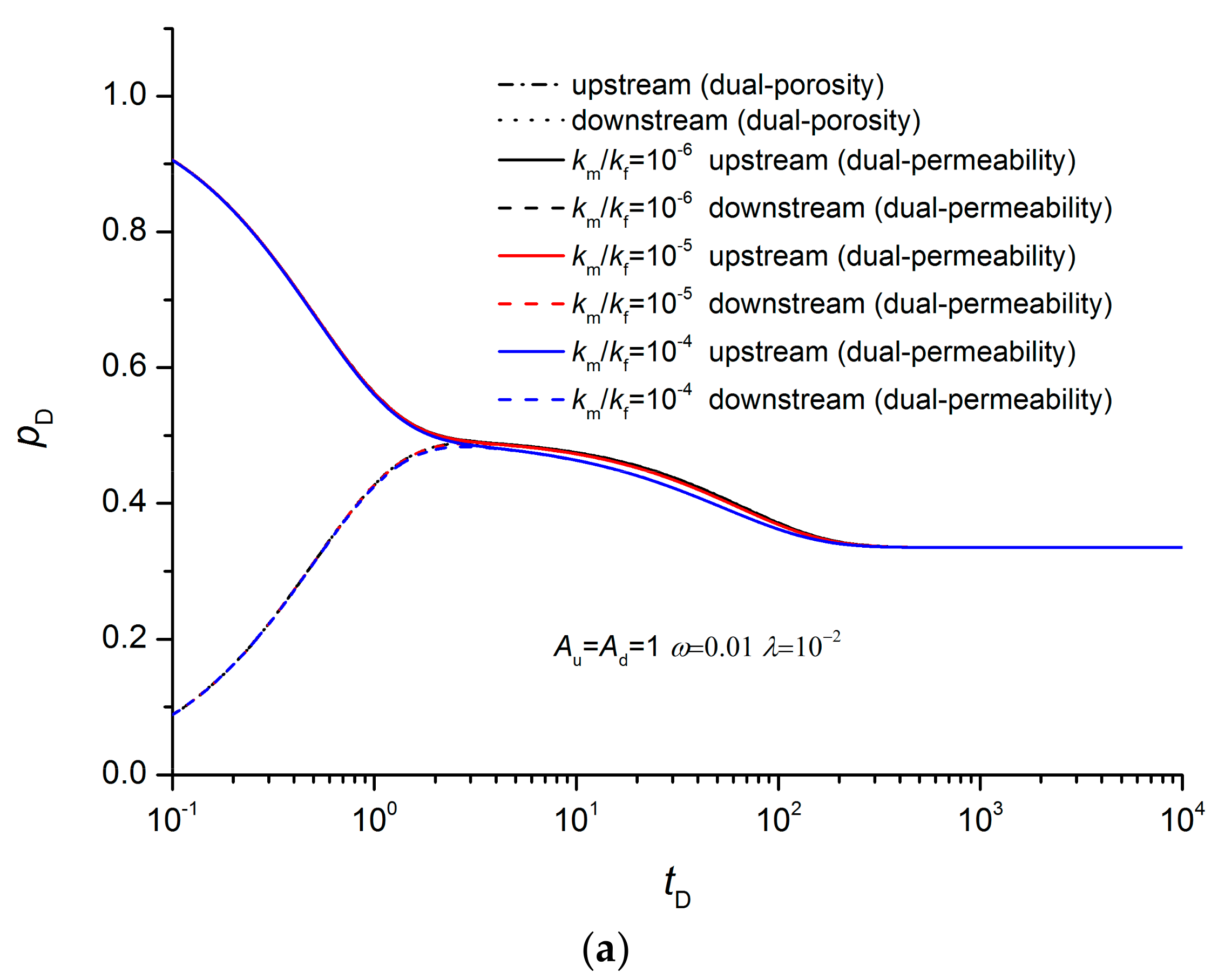
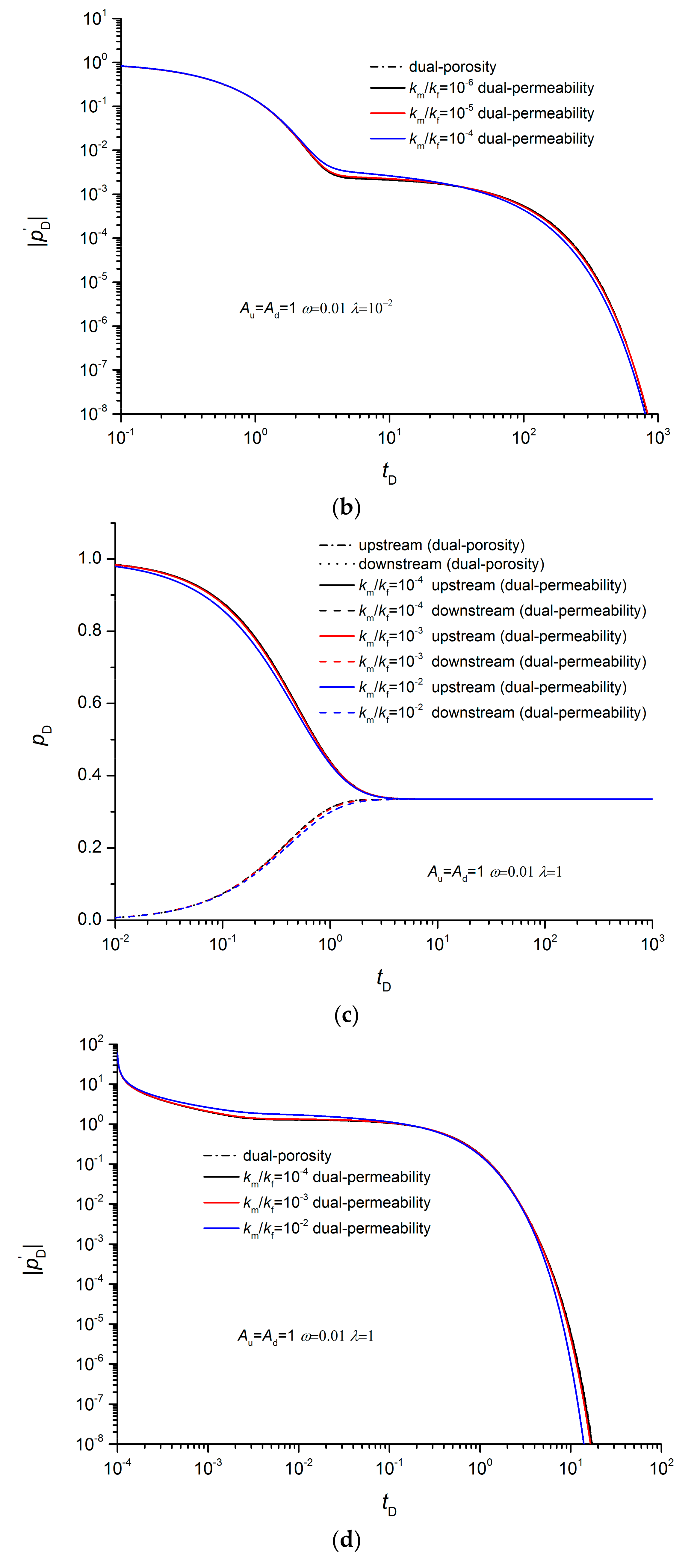
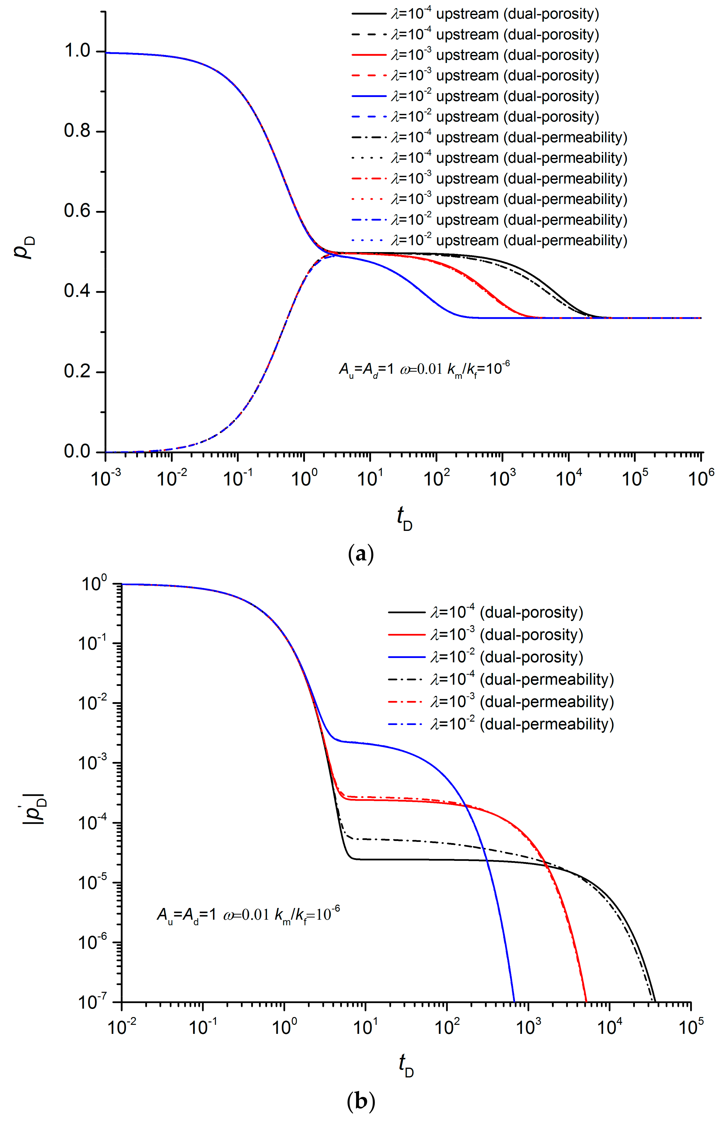
The numerical modeling results of pulse decay tests for dual-permeability and dual-porosity models with different matrix-fracture permeability ratios are shown in Figure 8. When the interporosity flow coefficient is small (λ = 0.01), the pressure and pressure derivatives of the two models coincide in the early (t_D < 1) and equilibrium (t_D > 10³) stages, and they only have a slight difference in the interporosity flow (1 < t_D < 10³) stage. When the matrix-fracture permeability ratio is less than 10⁻⁵, the results of the two models coincide substantially. If the interporosity flow coefficient is large (λ = 1), the interporosity flow occurs in the early stage (t_D < 1), and the matrix-fracture permeability has the same effect on the pressure and pressure derivative as the interporosity flow coefficient is small. Only when the value is less than 10⁻³ do the pressure and pressure derivative curves coincide for the two models. Even when the results of the two models do not completely coincide, their difference is very small. Therefore, when the matrix-fracture permeability ratio is less than 10⁻², the difference between the dual-permeability and dual-porosity models can be ignored.

4.4. Effect of Interporosity Flow Coefficient

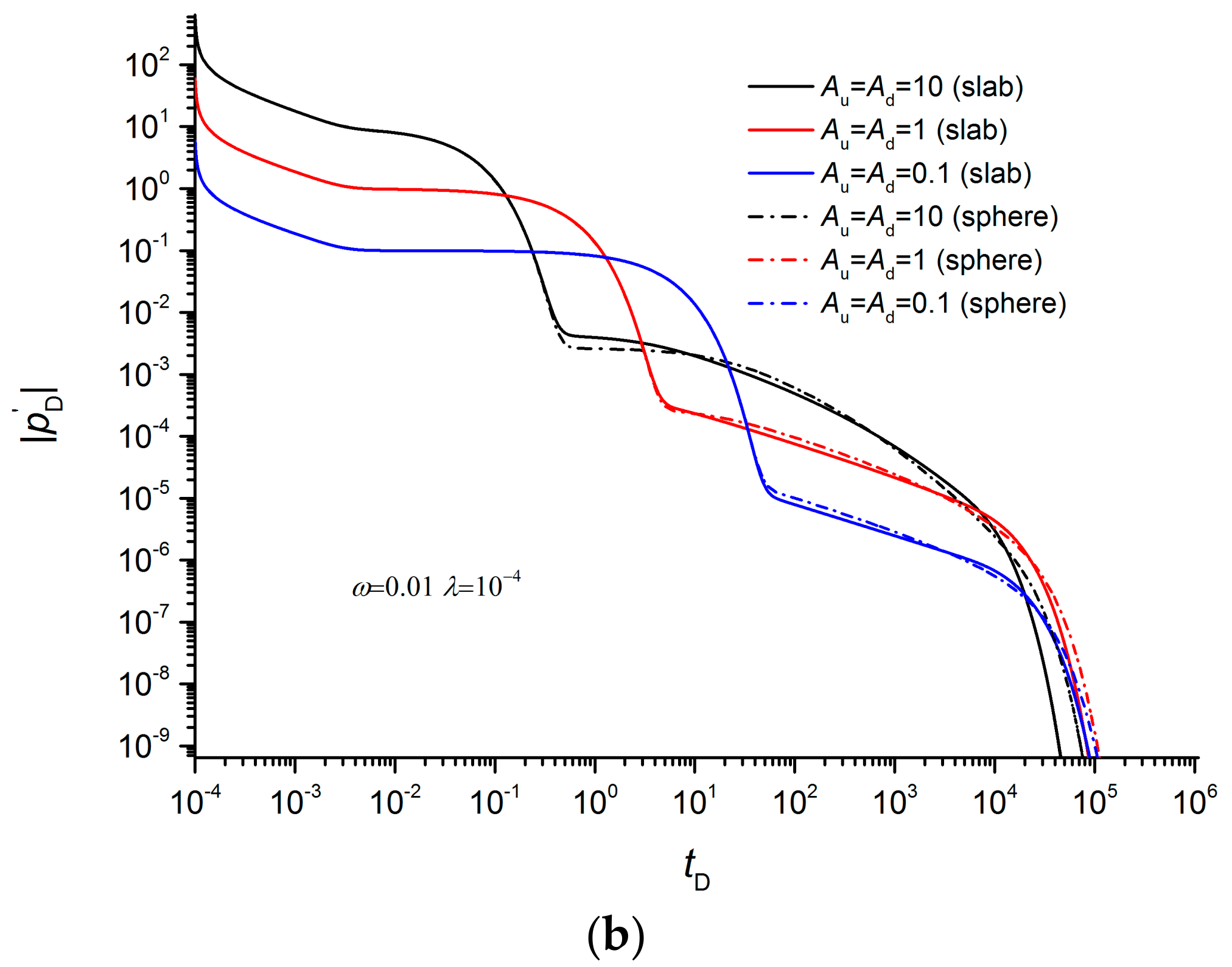
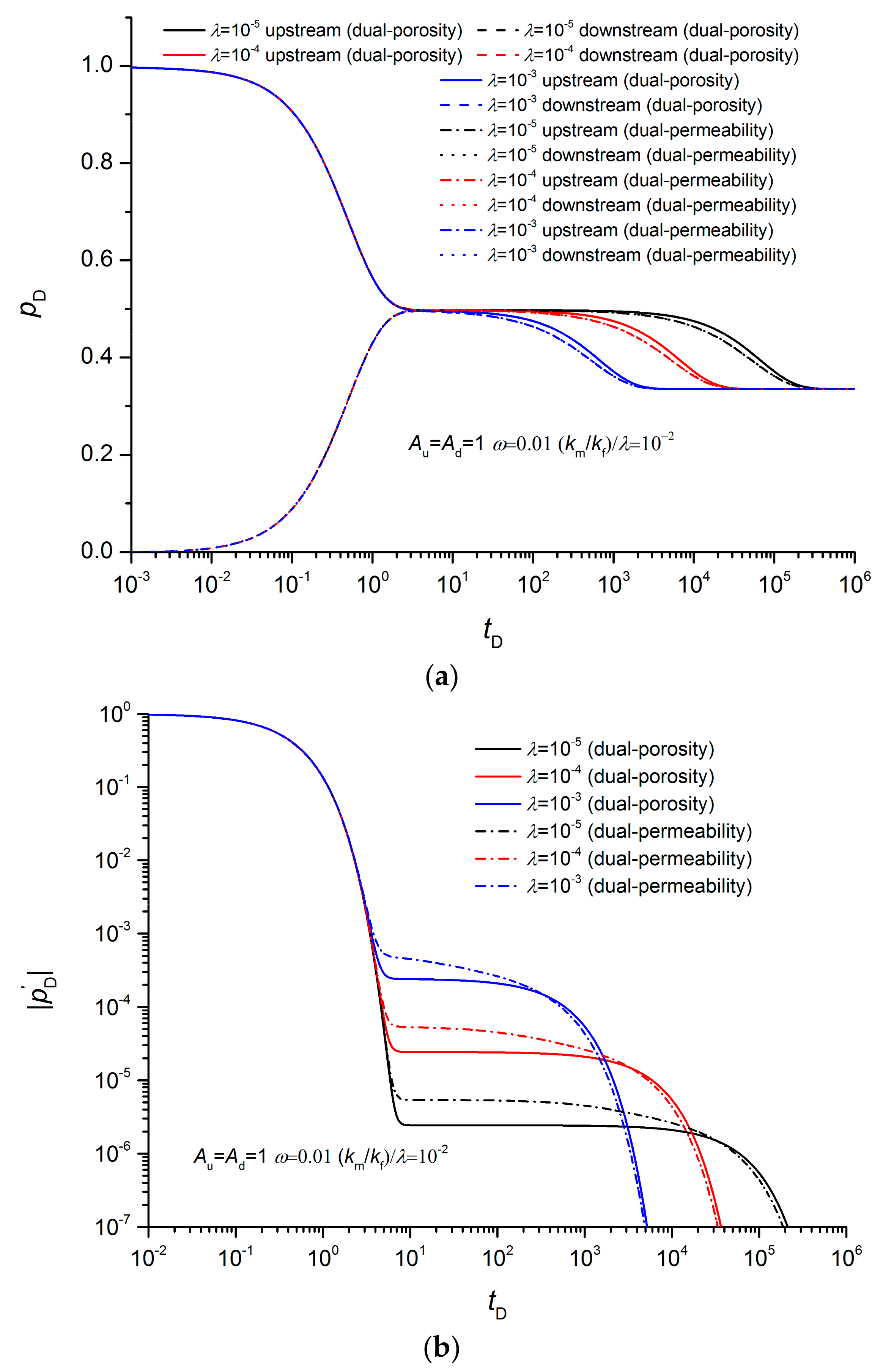
The numerical modeling results of pulse decay tests for dual-permeability and dual-porosity cores with different interporosity flow coefficients are shown in Figure 9 and Figure 10. In the early (t_D < 1) and equilibrium (for λ = 10⁻⁴, t_D > 10⁵) stages, the pressure and pressure derivatives of the dual-porosity and dual-permeability cores coincide. Only during the interporosity flow (for λ = 10⁻⁴, 1 < t_D < 10⁵) stage, is there a difference. If the matrix-fracture permeability ratio remains the same, as the interporosity flow coefficient decreases, the difference between the two models becomes larger (Figure 9). When the interporosity coefficient is 10⁻², the pressure and pressure derivative curves of the two coincide. When the matrix structure remains constant, i.e., the shape factor α is constant, the interporosity flow coefficient does not affect the difference between the two models (Figure 10). When the interporosity flow coefficient (λ ≥ 10⁻³) is large, the horizontal derivative of the pressure derivative of the interporosity flow section of the dual-permeability model disappears, and the shape is closer to the pseudo-steady-state interporosity flow model.

5. Case Studies

Han et al. (2018) [29] used the slab matrix dual-porosity model to fit the experimental data of Cronin (2014) [23] and obtained good results. In this study, the fitting parameters of Han et al. (2018) [29] were used. The pulse decay test was simulated based on the sphere matrix dual-porosity model and the dual-permeability model. The comparison of results with the test data is shown in Figure 11. Although the same set of parameters is used, all three models can obtain good fitting results. Their fittings are slightly different in the interporosity flow stage, and the fitting of the sphere matrix dual-porosity model is slightly better. However, this fitting does not mean that the core matrix is close to a sphere because the CT scan for the core shows that the core is stratified by alternating high- and low-density layers [23]. It can be deduced that the shape of the matrix cannot be inferred by the pulse decay test result. The low-density layer is approximately 4 to 8 mm thick, and the high-density layer is approximately 6 to 12 mm thick [23]. Assuming the permeability of the high-density layers is lower, the low permeability layer accounts for 60% of the cross-section. The average permeability of the high permeability layer measured by Cronin (2014) [23] is 9.2 × 10⁻²⁰ m², and the permeability of the low permeability layer is presumed to be 2.8 × 10⁻²³ m². From this, we can estimate that the average permeability of the low-permeability layer is 1.6 × 10⁻²³ m². Therefore, the low-high permeability ratio k_m/k_f ≈ 1.8 × 10⁻⁴ can be obtained. However, k_m/k_f = 2.0×10⁻⁴ was used in the numerical modeling. Note that in this case, when k_m/k_f is on the order of 10⁻⁴, k_m/k_f has little effect on the simulation results within a multiple variations. Therefore, the dual-permeability model can obtain the magnitude of the permeability ratio of the high and low permeability layers.

6. Summary and Conclusions

Comparative analysis of pressure and pressure derivative curves for pulse decay tests was carried out. The performance differences between dual-permeability and dual-porosity models and between sphere and slab matrix transient dual-porosity cores were studied under different vessel volumes, storativity ratios, matrix-fracture permeability ratios, and interporosity flow coefficients. The results are summarized as follows:

• The pressure and pressure derivative curves of sphere and slab matrix transient dual-porosity cores are coincident in early and equilibrium stages and are slightly different in the interporosity flow stage.
• Since the values and shapes of the pressure and pressure derivative curves are very similar, it is difficult to distinguish between the two matrix shapes, and another observation is necessary to estimate the matrix shape.
• The pressure and pressure derivative curves of dual-permeability and dual-porosity models are coincident in the early and equilibrium stages and are slightly different in the interporosity flow stage.
• Compared with the dual-porosity model, the horizontal section of the pressure derivative in the interporosity flow stage of the dual-permeability model is shorter.
• When the interporosity flow coefficient or vessel volume is large, the dual-permeability model is close to the pseudo-steady-state model.
• When the matrix-fracture permeability ratio is less than 10⁻², the difference between the dual-permeability model and the dual-permeability model can be ignored.
• The results of fitting the three models against the experimental data verify the results of this study.

When the core contains only a few fractures to the core scale, although it often exhibits similar characteristics of the dual-continuum medium, the dual-continuum medium model is not very accurate, and the discrete fracture model is more suitable. This study conducted a comprehensive comparative analysis of all parameters of various dual-continuum medium models for pulse decay tests. Not only their pressure curves were compared but also their pressure derivative curves. However, only one test case was used to verify the results of this study. It is hoped that there will be more experimental data to verify the conclusions in the future.

References

- Zhang, L.; Kou, Z.; Wang, H.; Zhao, Y.; Dejam, M.; Guo, J.; Du, J. Performance analysis for a model of a multi-wing hydraulically fractured vertical well in a coalbed methane gas reservoir. J. Pet. Sci. Eng. 2018, 166, 104–120. [Google Scholar] [CrossRef]
- Wei, M.; Dong, M.; Fang, Q.; Dejam, M. Transient production decline behavior analysis for a multi-fractured horizontal well with discrete fracture networks in shale gas reservoirs. J. Porous Media 2019, 22, 343–361. [Google Scholar] [CrossRef]
- Dejam, M.; Hassanzadeh, H.; Chen, Z. Semi-analytical solution for pressure transient analysis of a hydraulically fractured vertical well in a bounded dual-porosity reservoir. J. Hydrol. 2018, 565, 289–301. [Google Scholar] [CrossRef]
- Dejam, M.; Hassanzadeh, H.; Chen, Z. Pre-Darcy flow in porous media. Water Resour. Res. 2017, 53, 8187–8210. [Google Scholar] [CrossRef]
- Brace, W.F.; Walsh, J.B.; Frangos, W.T. Permeability of granite under high pressure. J. Geophys. Res. 1968, 73, 2225–2236. [Google Scholar] [CrossRef]
- Hsieh, P.A.; Tracy, J.V.; Neuzil, C.E.; Bredehoeft, J.D.; Silliman, S.E. A transient laboratory method for determining the hydraulic properties of ‘tight’ rocks—I. Theory. Int. J. Rock Mech. Min. Sci. Geomech. Abstr. 1981, 18, 245–252. [Google Scholar] [CrossRef]
- Jones, S.C. A technique for faster pulse-decay permeability measurements in tight rocks. SPE Form. Eval. 1997, 12, 19–25. [Google Scholar] [CrossRef]
- Jang, H.; Lee, W.; Kim, J.; Lee, J. Novel apparatus to measure the low-permeability and porosity in tight gas reservoir. J. Pet. Sci. Eng. 2016, 142, 1–12. [Google Scholar] [CrossRef]
- Zhao, Y.; Zhang, L.; Wang, W.; Tang, J.; Lin, H.; Wan, W. Transient pulse test and morphological analysis of single rock fractures. Int. J. Rock Mech. Min. Sci. 2017, 91, 139–154. [Google Scholar] [CrossRef]
- Metwally, Y.M.; Sondergeld, C.H. Measuring low permeabilities of gas-sands and shales using a pressure transmission technique. Int. J. Rock Mech. Min. Sci. 2011, 48, 1135–1144. [Google Scholar] [CrossRef]
- Cao, C.; Li, T.; Shi, J.; Zhang, L.; Fu, S.; Wang, B.; Wang, H. A new approach for measuring the permeability of shale featuring adsorption and ultra-low permeability. J. Nat. Gas Sci. Eng. 2016, 30, 548–556. [Google Scholar] [CrossRef]
- Dicker, A.I.; Smits, R.M. A practical approach for determining permeability from laboratory pressure-pulse decay measurements. In Proceedings of the SPE International Meeting on Petroleum Engineering, Tianjin, China, 1–4 November 1988. [Google Scholar] [CrossRef]
- Cui, X.; Bustion, A.M.M.; Bustion, R.M. Measurements of gas permeability and diffusivity of tight reservoir rocks: Different approaches and their applications. Geofluids 2009, 9, 208–223. [Google Scholar] [CrossRef]
- Kaczmarek, M. Approximate Solutions for Non-stationary Gas Permeability Tests. Transp. Porous Med. 2008, 75, 151–165. [Google Scholar] [CrossRef]
- Feng, R.; Liu, J.; Chen, S.; Bryant, S. Effect of gas compressibility on permeability measurement in coalbed methane formations: Experimental investigation and flow modeling. Int. J. Coal Geol. 2018, 198, 144–155. [Google Scholar] [CrossRef]
- Lin, Y.; Myers, M.T. Impact of non-linear transport properties on low permeability measurements. J. Nat. Gas Sci. Eng. 2018, 54, 328–341. [Google Scholar] [CrossRef]
- Alnoaimi, K.R.; Duchateau, C.; Kovscek, A.R. Characterization and measurement of multiscale gas transport in shale-core samples. SPE J. 2016, 21, 573–588. [Google Scholar] [CrossRef]
- Aljamaan, H.; Ismail, M.A.; Kovscek, A.R. Experimental investigation and Grand Canonical Monte Carlo simulation of gas shale adsorption from the macro to the nano scale. J. Nat. Gas Sci. Eng. 2017, 48, 119–137. [Google Scholar] [CrossRef]
- Bhandari, A.R.; Flemings, P.B.; Polito, P.J.; Cronin, M.B.; Bryant, S.L. Anisotropy and Stress Dependence of Permeability in the Barnett Shale. Transp. Porous Med. 2015, 108, 393–411. [Google Scholar] [CrossRef]
- Kamath, J.; Boyer, R.E.; Nakagawa, F.M. Characterization of core-scale heterogeneities using laboratory pressure transients. SPE Form. Eval. 1992, 7, 219–227. [Google Scholar] [CrossRef]
- Ning, X.; Fan, J.; Holditch, S.A.; Lee, W.J. The measurement of matrix and fracture properties in naturally fractured cores. In Proceedings of the Low Permeability Reservoirs Symposium, Denver, CO, USA, 26–28 April 1993. [Google Scholar] [CrossRef]
- Cronin, M.B.; Flemings, P.B.; Bhandari, A.R. Dual-permeability microstratigraphy in the Barnett Shale. J. Pet. Sci. Eng. 2016, 142, 119–128. [Google Scholar] [CrossRef]
- Cronin, M.B. Core-Scale Heterogeneity and Dual-Permeability Pore Structure in the Barnett Shale. Ph.D. Thesis, The University of Texas at Austin, Austin, TX, USA, December 2014. [Google Scholar]
- Liu, H.; Lai, B.; Chen, J.; Georgi, D. Pressure pulse-decay tests in a dual-continuum medium: Late-time behavior. J. Pet. Sci. Eng. 2016, 147, 292–301. [Google Scholar] [CrossRef]
- Jia, B.; Tsau, J.S.; Barati, R. Evaluation of core heterogeneity effect on pulse-decay experiment. In Proceedings of the International Symposium of the Society of Core Analysts, Vienna, Austria, 27 August–1 September 2017. [Google Scholar]
- Jia, B.; Tsau, J.; Barati, R. Experimental and numerical investigations of permeability in heterogeneous fractured tight porous media. J. Nat. Gas Sci. Eng. 2018, 58, 216–233. [Google Scholar] [CrossRef]
- Alnoaimi, K.R.; Kovscek, A.R. Influence of microcracks on flow and storage capacities of gas shales at core scale. Transp. Porous Med. 2019, 127, 53–84. [Google Scholar] [CrossRef]
- Bajaalah, K.S. Determination of Matrix and Fracture Permeabilities in Whole Cores Using Pressure Pulse Decay. Master’s Thesis, King Fahd University of Petroleum and Minerals, Dhahran, Saudi Arabia, June 2009. [Google Scholar]
- Han, G.; Sun, L.; Liu, Y.; Zhou, S. Analysis method of pulse decay tests for dual-porosity cores. J. Nat. Gas Sci. Eng. 2018, 59, 274–286. [Google Scholar] [CrossRef]
- Warren, J.E.; Root, P.J. The Behavior of Naturally Fractured Reservoirs. SPE J. 1963, 3, 245–255. [Google Scholar] [CrossRef] [Green Version]
- Bourdet, D.; Johnston, F. Pressure bevhavoir of layered reservoirs with crossflow. In Proceedings of the SPE 1985 California Regional Meeting, Bakersfield, CA, USA, 27–29 March 1985. [Google Scholar] [CrossRef]
Figure 1.
Schematic diagram of the apparatus for pulse decay tests.
Figure 2.
Schematic diagram of flow characteristics for dual-continuum medium models. (a) dual-porosity model. (b) dual-permeability model. (The blue arrows indicate the interporosity flow. The red arrows indicate the flow pathway of the system.).
Figure 3.
Effect of vessel volume on the pulse decay test for dual-porosity cores. (a) Pressure history. (b) Pressure derivative.
Figure 4.
Effect of storativity ratio on pulse decay tests for dual-porosity cores. (a) Pressure history. (b) Pressure derivative.
Figure 5.
Effect of interporosity flow coefficient on pulse decay tests for dual-porosity cores. (a) Pressure history. (b) Pressure derivative history.
Figure 6.
Effect of vessel volumes on pulse decay tests for dual-permeability. (a) Pressure history. (b) Pressure derivative history.
Figure 7.
Effect of the storativity ratio on pulse decay tests for dual-permeability cores. (a) Pressure history. (b) Pressure derivative history.
Figure 8.
Effect of matrix-fracture permeability ratio on pulse decay tests for dual-permeability cores. (a) Pressure history for λ = 0.01. (b) Pressure derivative history λ = 0.01. (c) Pressure history for λ = 1. (d) Pressure derivative history for λ = 1.
Figure 9.
Effect of the interporosity flow coefficient on pulse decay tests for dual-permeability cores (fixed matrix-fracture permeability ratio). (a) Pressure history. (b) Pressure derivative history.
Figure 10.
Effect of interporosity flow coefficients on pulse decay test for dual-permeability cores (fixed matrix structure). (a) Pressure history. (b) Pressure derivative history.
Figure 11.
Comparison between the numerical modeling results and experimental data of Cronin (2014) for (a) pressure histories and (b) pressure derivative histories.