CFD Simulations on the Rotor Dynamics of a Horizontal Axis Wind Turbine Activated from Stationary


1
Department of Mechanical Engineering, Chung Yuan Christian University, Chung Li, Taoyuan City 32023, Taiwan
2
Department of Mechanical Engineering, Wu Feng University, Minhsiung, Chiayi County 62153, Taiwan
3
Department of Mechatronic Engineering, Institute of Mechanical and Electrical Engineering, Lingnan Normal University, Zhanjiang 524048, Guangdong, China
*
Authors to whom correspondence should be addressed.
Appl. Mech. 2021, 2(1), 147-158; https://0-doi-org.brum.beds.ac.uk/10.3390/applmech2010009
Submission received: 6 February 2021
/
Revised: 26 February 2021
/
Accepted: 1 March 2021
/
Published: 5 March 2021
Abstract
:The adaptive dynamic mesh, user-defined functions, and six degrees of freedom (6DOF) solver provided in ANSYS FLUENT 14 are engaged to simulate the activating processes of the rotor of the Grumman WS33 wind system. The rotor is activated from stationary to steady operation driven by a steady or periodic wind flow and its kinematic properties and power generation during the activating processes. The angular velocity and angular acceleration are calculated directly by the post-processed real-time 6DOF solver without presuming a known rotating speed to the computational grid frame. The maximum angular velocity of the rotor is approximately proportional to the driving wind speed, and its maximal angular acceleration is also closely proportional to the square of the driving wind speed. The evolution curves of the normalized rotor angular velocities and accelerations are almost identical due to the self-similarity properties of the rotor angular velocities and accelerations. The angular velocity of the rotor will reach its steady value. One can use these steady angular velocities to predict the mechanical power generations of the rotor. The momentum analysis theory and the blade element momentum method are applied to predicted power generations and reveal good agreements with experimental data in the low wind speed range.
1. Introduction
Power generation by oil and coal is currently the primary energy/electricity source globally, and a tremendous amount of carbon dioxide is produced during power generating processes, which increases global warming and extreme weather due to the greenhouse effect. Therefore, many countries actively legislate laws and regulations to reduce carbon dioxide generation and suspended particulate matter. Meanwhile, renewable energies are developed constructively to replace or reduce the use of fossil fuels, and the technology of power generation by wind energy is one of the foci.
When the aerodynamic properties of a wind turbine rotor are revealed, engineers can evaluate the mechanical power generation of the rotor, the stresses of blades induced by air pressure, and the flow field surrounding the rotor blade. Theoretically, the momentum analysis theory [1] and the blade element momentum (BEM) method [2] provide tools to estimate the performance of a wind turbine rotor. However, when applying those two theories, one has to assign a constant inflow wind speed. The BEM method could combine the tip loss and wake flow of the blade and then predict the aerodynamic performances of rotors [3,4,5,6].
In a real scenario, a wind turbine is driven usually by an unsteady wind field. This unsteady wind field will affect the aerodynamic characteristics, vortex formation, wake flow, and the energy transformation efficiency of a wind turbine. The unsteady BEM method [2] is a useful tool to determine how the unsteady wind field affects a wind turbine rotor. Huyer et al. [7] studied the transient aerodynamics of several kinds of horizontal axis wind turbines and found that the magnitude of the normal force on the tip or 30–60% of the wingspan of a blade is two times the normal force obtained in a steady flow field. To enhance the numerical analysis efficiency, Xu and Sankar [8] divided the computational domain into two subdomains: the Navier–Stokes subdomain near the rotor and the outer potential flow subdomain region. The numerical simulation results obtained with this hybrid computational domain using the BEM method were compared with the experimental results. Wright and Wood [9] analyzed the aerodynamic characteristics of a blade by the BEM method with the data from a quasi-steady operated wind turbine, and the predicted results were very close to the experimental data of some types of wind turbines. Silva and Donadon [10] developed a numerical scheme that combines the unsteady BEM method, returning wake effects, and hybrid computational domain [8] to reveal the wake flows of rotor blades and obtained reasonable predictions. De Freitas Pinto and Gonçalves [11] derived a fourth-order linear equation by combining the BEM method and momentum analysis to obtain analytic solutions of the aerodynamic characteristics of wind turbine blades. Their study indicated that the maximal power efficiency, 16/27, predicted by Betz, is impossible to achieve because the tip speed ratio has to be infinity. El khchine and Sriti [12] also proposed an equation, with the BEM method, to describe the correlation between tangential and axial induction factors (lift/drag ratio) and tip speed ratio. This equation can promote the accuracy of the prediction.
Numerical computation programs allow engineers and professionals to predict the aerodynamic properties, vortex formation, and wake flow of a wind turbine rotor. Constant inflow wind speeds and the computational meshes constructed in a moving reference frame (MRF) are applied frequently during the numerical simulation processes. The MRF is a frame that rotates about a fixed axis with a constant angular velocity, which is obtained from experimental results or given by researchers. In this frame, the problem of a rotating rotor with constant angular velocity and wind speed transforms into that of a fixed rotor driven by a constant rotating wind field. Then, the wind field surrounding the rotor is modeled as a steady-state problem for the rotor, as suggested in the ANSYS FLUENT 14 Theory Guide [13]. This methodology is prevalent in two- or three-dimensional numerical simulation analysis by ANSYS or other numerical programs. Gupta and Biswas [14] analyzed the performance of a twisted three-bladed H-Darrieus rotor. They constructed their numerical model by unstructured meshes and an MRF provided by FLUENT 6.2. They compared the validation of the aerodynamics coefficients predicted by their numerical simulations with their experimental data. Lanzafame, Mauro, and Messina [15] developed a 3D numerical simulation model of a horizontal-axis wind turbine (HAWT) using ANSYS FLUENT. A moving reference frame was applied to simulate the rotation of the rotor blades. Sudhamshu et al. [16] studied how a pitch angle affects the performance of an HAWT. ANSYS FLUENT was applied to obtain the results. The computational domain was constructed in an MRF. Shu et al. [17] estimated the aerodynamic performance of a rotor blade after icing. They also used the ANSYS FLUENT code to make their 3D numerical simulation, and the multiple reference frame (one of the MRFs) was chosen to describe the rotor rotating steadily. Torregrosa et al. [18] proposed an enhanced design methodology of a low-power stall-regulated wind turbine. The commercial package STAR CCM+ was used to simulate the 3D effects of the rotor blades. The governing equations were solved in an MRF. Rodrigues and Lengsfeld [19,20] developed a numerical prediction to improve wind farm layout. To solve situations involving moving, ANSYS FLUENT was applied with an MRF.
The studies mentioned above focused on the aerodynamic functions of wind turbine rotors in a steady or unsteady wind field. However, the ANSYS FLUENT 14 Theory Guide suggests that researchers can employ dynamic meshes to capture the transient flow field of the rotor if the unsteady interaction between the stationary parts and moving parts is significant. Nevertheless, the passive rotation-activating process of the wind turbine rotor from stationary to steady operation by constant or unsteady wind speeds is seldom mentioned. Additionally, with the transient rotational object and/or unsteadiness of the wind field, the aerodynamic equivalence applicability in previous CFD flow simulation methodologies, such as MRF, is still in doubt. Therefore, the kinematic behaviors and the mechanical power generation of the rotor during the activating processes need to be discussed.
In the present study, a numerical simulation model is established based on the configuration of the rotor of the Grumman WS33 wind system [21], which is chosen as a sample task to demonstrate the ideology of passive CFD simulation without using the MRF scheme. The adaptive dynamic meshes and user-defined functions (UDFs) provided by ANSYS FLUENT 14 are engaged in simulating the activating process of the rotor. The rotational properties are obtained from a post-processed real-time six degrees of freedom (6DOF) solver for the wind turbine rotor by solving the solid–fluid interaction of the dynamic meshes. The significant advantage of the present numerical methodology is that the measured or empirically estimated angular velocity and the rotational torque of the rotor are not required numerical simulation conditions. The transient angular velocity and angular acceleration are calculated directly within the computing processes. Additionally, the mechanical power generation of the rotor can be promptly predicted by momentum analysis and the BEM method with the data obtained from the present simulations. Furthermore, these predicted results are compared with the measured data of the Grumman Stream 33 wind turbine system presented in previous studies.
2. Modeling and Methods
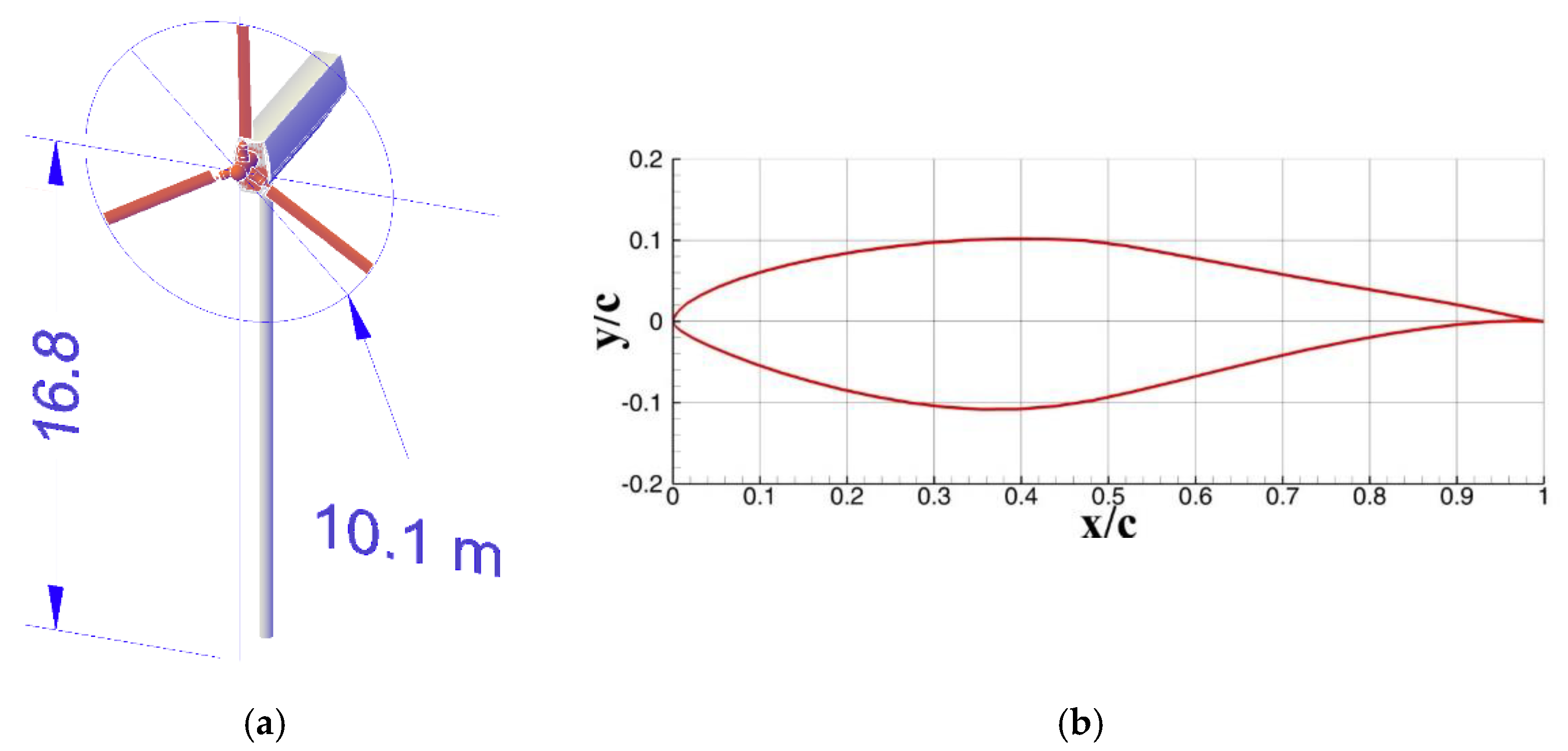
The rotor diameter of the Grumman Wind Stream 33 wind turbine is 10.1 m, denoted as D, and there are three blades on the rotor, as shown in Figure 1. The airfoil of the blade is S809 [21], with a chord length of 0.4571 m and a wingspan length of 4.3 m [5,6].
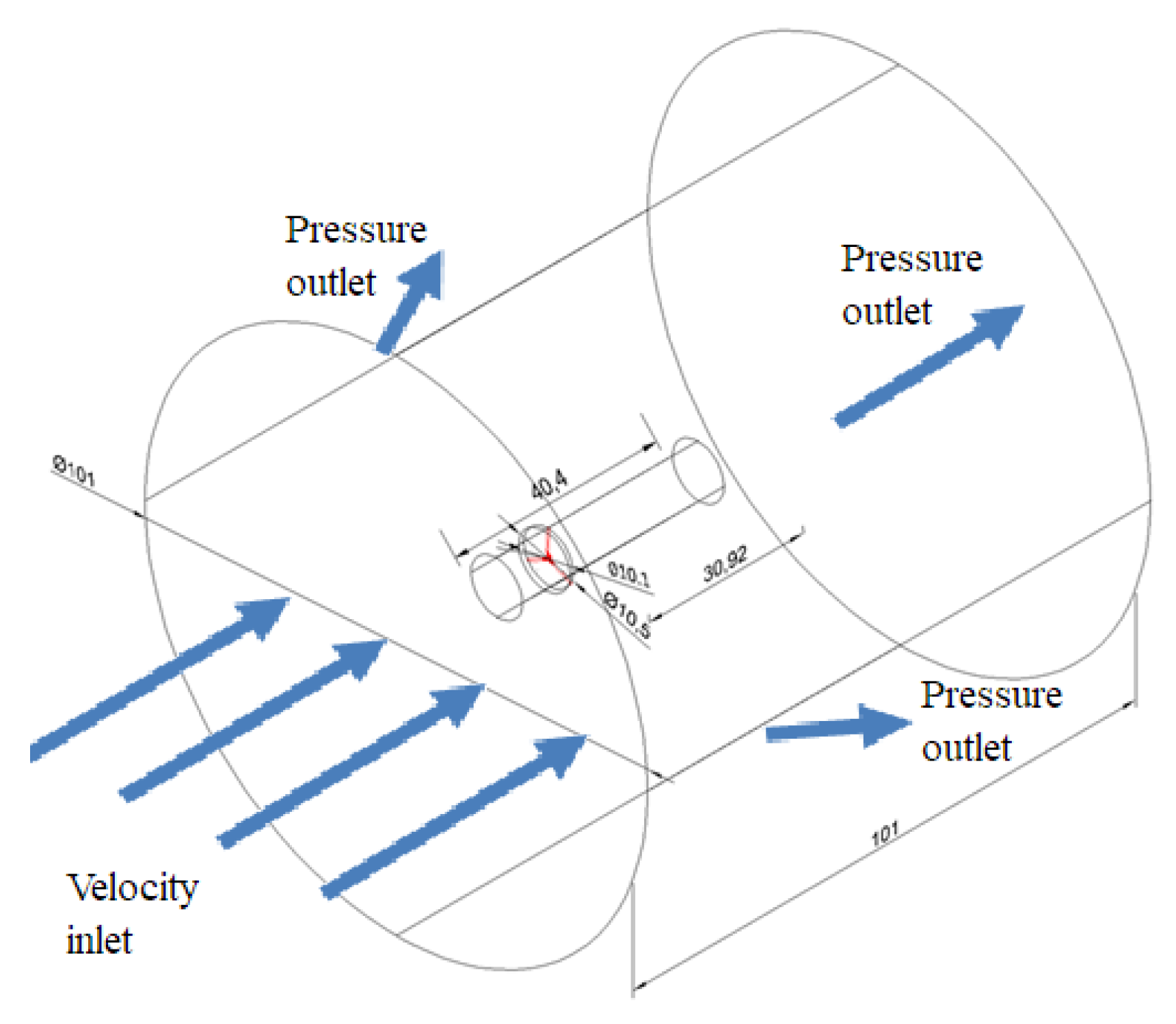
The computational meshes were generated in a cylindrical domain. The longitudinal length and the diameter of the cylindrical computational domain were 10D (101 m, 1D = 10.1 m). The rotor was placed on the central axis of the cylindrical space at the location 3D (30.3 m) behind the flow entrance surface. Furthermore, the computational domain was divided into two subdomains to save computer resources and reduce the computing time. Meanwhile, the dynamic meshes were assigned in the inner subdomain near the rotor. The inner subdomain diameter was 1D, and the longitudinal length was 4D (1D in front of the rotor and 3D behind). The fixed meshes were assigned to the outer subdomain. A schematic diagram of the computational domain is presented in Figure 2.
The working fluid was air, and the flow status was turbulent. The turbulent model assigned in ANSYS FLUENT 14 is the model, which is suitable for high Reynolds number conditions. In the present study, the range of the Reynolds number of the air was from 1.42 × 10⁵ (the wind speed is 10 mph 4.47 m/s) to 4.9 × 10⁵ (the wind speed is 35 mph 15.65 m/s). Boundary conditions were as follows: The front surface was subject to a uniform steady or unsteady velocity inflow, and rare and lateral surfaces were set up to zero gauge pressure in the outlet (the reference pressure was one standard atmospheric pressure, 1 atm). The types and signs of the boundary conditions are also illustrated in Figure 2. The formulation of wind velocity fluctuation was inspired by the offshore wind study conduct by Kondo, Fujinawa, and Naito [22] and the metrology records in [23]. One can conclude that the average magnitude of wind speed fluctuation is about 14% of its mean value. Therefore, the periodic wind speed can be described as follows:
where , , and are the mean wind speed, period of fluctuation, and operating time, respectively.
As mentioned above, the rotor was initially stationary and activated passively by a steady or periodic oscillating wind field. The rotating speed of the rotor was not always constant during the simulation time interval. Therefore, the MRF was not a proper moving frame to simulate the activating process we wished to engage in, as suggested in the ANSYS FLUENT Theory Guide [13]. The adaptive dynamic meshes with UDFs, provided by ANSYS FLUENT 14, matched the requirement of this situation. UDFs define the steady or unsteady inflow wind speed conditions and the constraints used in CFD simulations, such as the mass, moment of inertia, etc. The 6DOF solver gives real-time results of the dynamic properties between the air and the rotor blade surface. Therefore, a presumed constant angular velocity of the rotor was not a necessary condition.
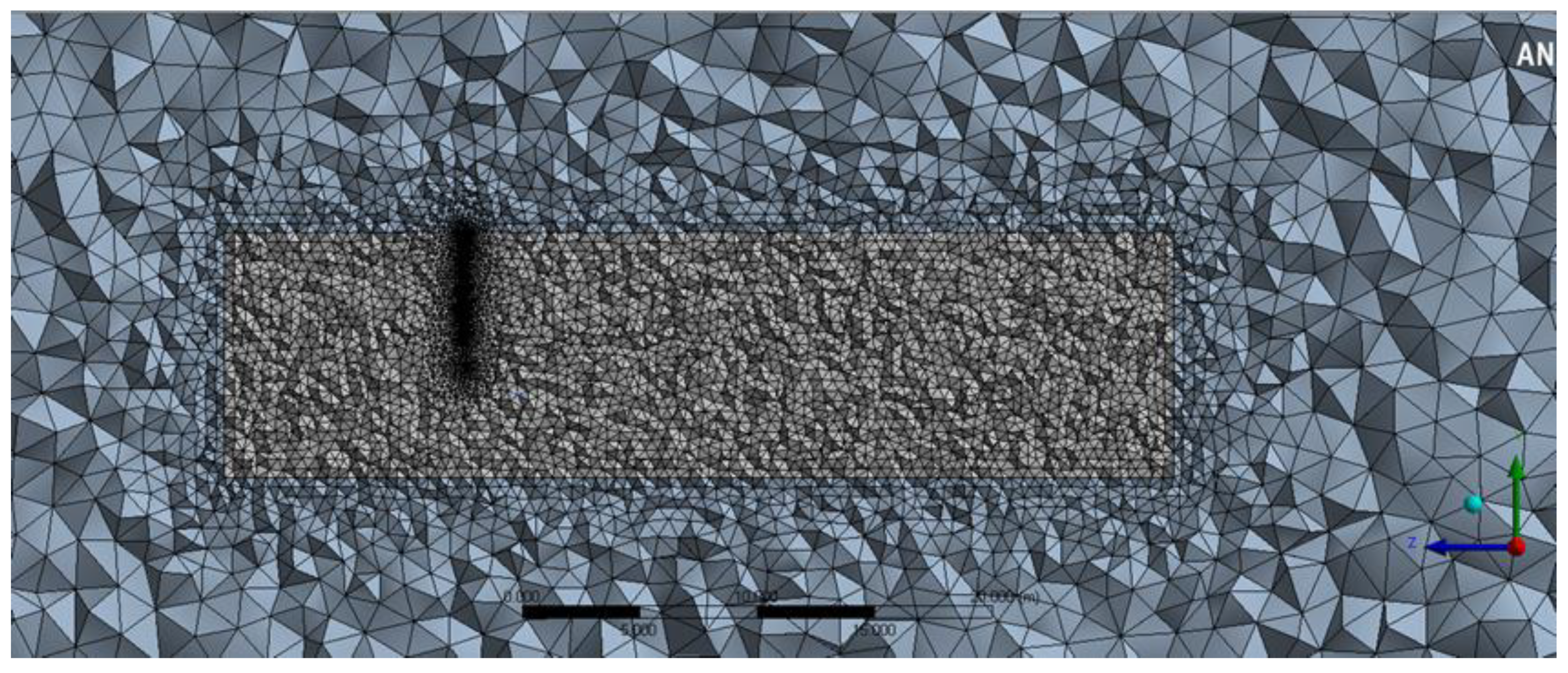
The top-central cross-sectional diagram of the mesh element distribution is shown in Figure 3. Non-structural meshes were generated automatically by ANSYS FLUENT 14, and the configuration of the mesh was tetrahedral. The maximal skewness of the meshes was less than 0.85. Due to the mesh convergence test, as shown in Table 1, the optimal total number of mesh elements was 689,820. The mesh setting for first layer thickness was 0.013 m and then with default growth of 1.2 times for further layers away from the wall. Such thickness value with varying wind speed translates into a range of 125 to 245 in terms of y+ (). The range is adequate for CFDs simulation with the turbulent model, and a standard wall function was enabled and used in the ANSYS initial setting, as its standard value is from 30 to 300.
To prevent failure adaption of the invalid volume of mesh from 6DOF motion by enabling dynamic meshes, the function of re-meshing and smoothing was also enabled from the dynamic mesh function panel in ANSYS FLUENT 14. A scheme of pressure–velocity coupling was used to faster achieve accurate pressure in the first timesteps of the simulation, as the rest of the scheme was changed to SIMPLE to save pressure evaluation at the last iteration of a time step. We performed an optimization for better computational efficiency.
3. Results
The kinematic properties of a rotor activated from stationary to steadily operating are presented first. The mean speed of the uniform driving wind field for simulation was 10, 15, 20, 25, 30, and 35 mph. The rotor operating time was 50 s, and the time step was 0.01 s for computational accuracy.
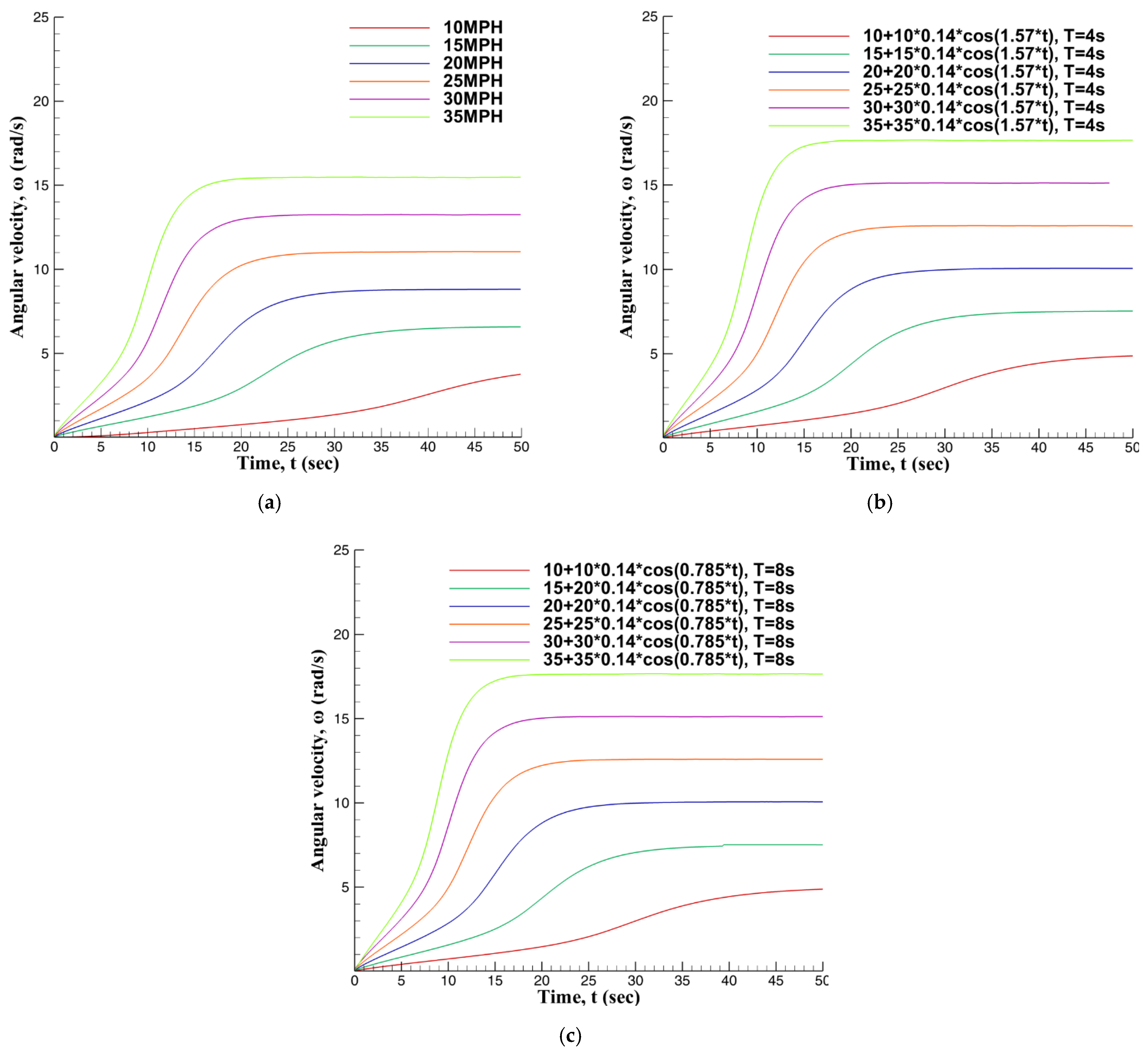
Figure 4a presents the evolution processes of the angular velocity of the rotor driven by steady uniform wind fields. One can observe that the faster the wind speed is, the sooner the rotor operates steadily with a higher angular velocity. The evolution processes of the angular velocity of the rotor driven by periodic wind fields, of which the oscillating period is 4 s, are shown in Figure 4b. Compared with the cases presented in Figure 4a, the rotor needs less time to reach a steady rotation, and the final angular velocity is higher than its counterpart in the steady wind field.
As shown in Table 2, because the maximal wind speed of the periodic wind field is 14% higher than the mean wind speed, the final steady angular velocity of the rotor also increases nearly to the value of 14%. For example, when the mean wind speed is 35 mph, the maximal angular velocity of the rotor driven by the steady wind field is about 15.2 rad/s, and in the periodic wind field is about 17.3 rad/s (17.3 ≈ 15.2 × 1.14). Meanwhile, the rotor driven by a periodic oscillating wind field takes a shorter time to reach its steady angular velocity than its counterpart in the steady wind field.
Figure 4c reveals the evolution processes of the angular velocity of the rotor driven by periodic wind fields, of which the oscillating period is 8 s. The evolution curves of the rotor angular velocities are almost identical to their counterparts shown in Figure 4b. One can conclude that the maximal driving wind speed is the critical factor affecting the activation processes of the rotor. However, the effects of the oscillating periods of the wind fields can be negligible during the activation processes.
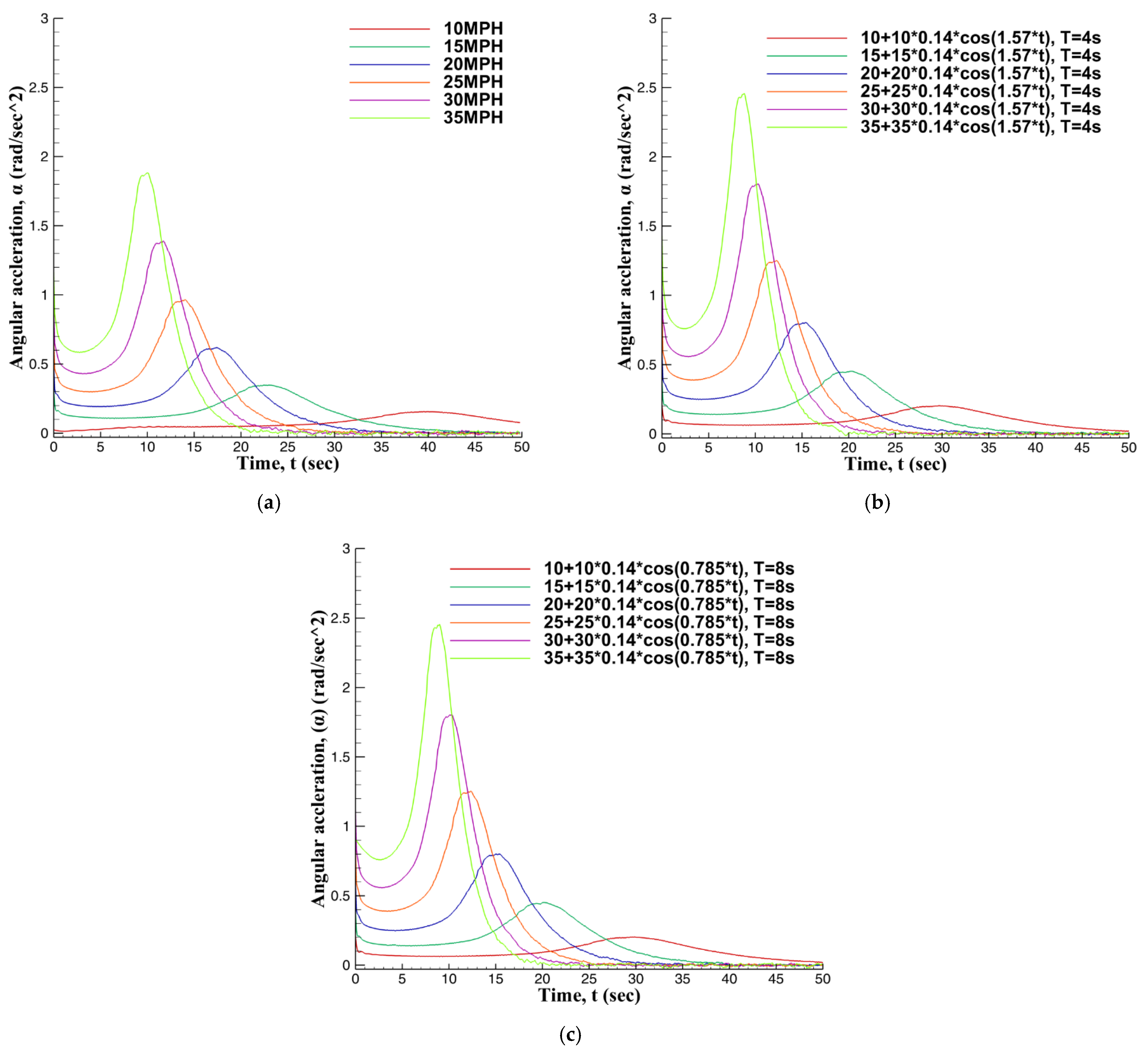
The evolution processes of the angular acceleration of the rotor driven by steady wind fields are presented in Figure 5a. It indicates that the higher the wind speed, the sooner the angular acceleration of the rotor reaches its maximal value and decays to zero. It means that the rotor can be easily activated and reaches a steady operating state, as shown in Figure 4a–c, when the speed of the driving wind field increases.
The evolution processes of the angular acceleration of the rotor driven by periodic wind fields, whose oscillating period is 4 s, are shown in Figure 5b. The curves of the evolutionary processes are similar to those counterparts presented in Figure 5a. As the maximal wind speed of each periodic wind field is 14% larger than the mean wind speed, the maximal angular acceleration of the rotor driven by the periodic wind field is about 1.142 times larger than its counterpart presented in Figure 5a. For instance, when the mean wind speed is 35 mph, the maximal angular acceleration of the rotor driven by the steady wind field is about 1.883 rad/s2, and by the periodic oscillating wind field is about 2.46 rad/s2 (2.46 ≈ 1.883 × 1.142).
As shown in Table 3, when the maximal wind speed of the periodic oscillating wind field is 14% larger than the mean wind speed, the maximal angular acceleration of the rotor raises approximately 1.142 times to its counterpart driven by the steady wind field. Meanwhile, the angular acceleration of the rotor driven by the periodic oscillating wind field reaches its maximum value earlier than its counterpart driven by the steady wind field.
Figure 5c reveals the evolution processes of the angular acceleration of the rotor driven by periodic wind fields, whose oscillating period is 8 s. It shows that the evolution curves of the angular acceleration are nearly identical to counterparts presented in Figure 5b. Similarly, it also reveals that the oscillating period of the periodic wind field does not affect the evolutionary processes of the angular acceleration of the rotor.
It seems that there are self-similarity properties of the rotor angular velocity and angular acceleration during the activating processes. Therefore, it indicates that some characteristic quantities could normalize the angular velocity, the angular acceleration, and the operation time. Thus, the curves of evolution processes could be re-plotted with those normalized quantities to show the self-similarity property. When a specific wind speed drives the rotor, the normalized angular velocity (normalized angular acceleration ) is said to be the ratio between the angular velocity (angular acceleration ) and the maximal angular velocity (maximal angular acceleration ):
Meanwhile, with corresponding wind speed, the normalized time is said to be the ratio between the rotor operating time and half of the time that the rotor takes to reach steady operation :
Figure 4 and Figure 5 could be re-plotted using the definitions of the normalized quantities shown in Figure 6. These figures indicate that self-similarity properties exist in the rotor angular velocity and angular acceleration processes when the driving wind speed is not the same. There are four stages in the normalized evolution processes, as follows:
- : The rotor starts to rotate and increases gently. Meanwhile, decreases initially and then increases. Then, reaches its local minimum of about 0.31 at the normalized time of 0.3.
- : increases rapidly, and increases to its maximal value of 1.0 at the normalized time of 1.07 and then decreases.
- : keeps decreasing, and the increasing rate of the normalized angular velocity slows down. The rotor is ready for steady operation.
- : The normalized angular velocity reaches its constant value, and the normalized angular acceleration decays to zero. The rotor operates steadily.
As shown in Figure 6, the self-similarity of the kinematic properties of the rotor during the activating processes is the first found phenomenon in the numerical simulation studies of the wind turbine rotors.
We do not consider the loadings of a rotor induced by other connected devices such as the shaft-bearing friction torque, gearbox, electric generator, etc. Therefore, our predicted angular velocities and angular accelerations of the rotor might be larger than those of a rotor operating in the real world. In previous studies, momentum analysis theory and the BEM method could estimate the power generation of a wind turbine rotor driven by a constant wind field. However, one cannot estimate the power generation of a rotor if the rotating dynamic properties of the rotor are unknown. Therefore, we can use both theories with our ANSYS simulation data to estimate the power generation of the rotor.
If the momentum analysis theory is applied to predict the torque of the rotor, one can set an adequate control volume to calculate the difference in the kinetic energy between the entry and the exit of the control volume. In the present study, the CFD-POST module of ANSYS is used to sketch more than 4000 streamlines in the computational domain shown in Figure 2. The data of the streamlines provide the variations in specific physical quantities in the flow streams.
The software Q-Blade can execute the calculations of the BEM method. The airfoil of each blade element is a given condition, and the blade elements are combined to form the whole blade of the rotor. Furthermore, the XFoil module can obtain the lift/drag coefficient of the blade under various angles of attack of wind. Then, the lift/drag coefficients are fed into Q-blade to find the force and torque of every single blade. The data that Q-blade needed were our ANSYS simulation data and the experimental data [6].
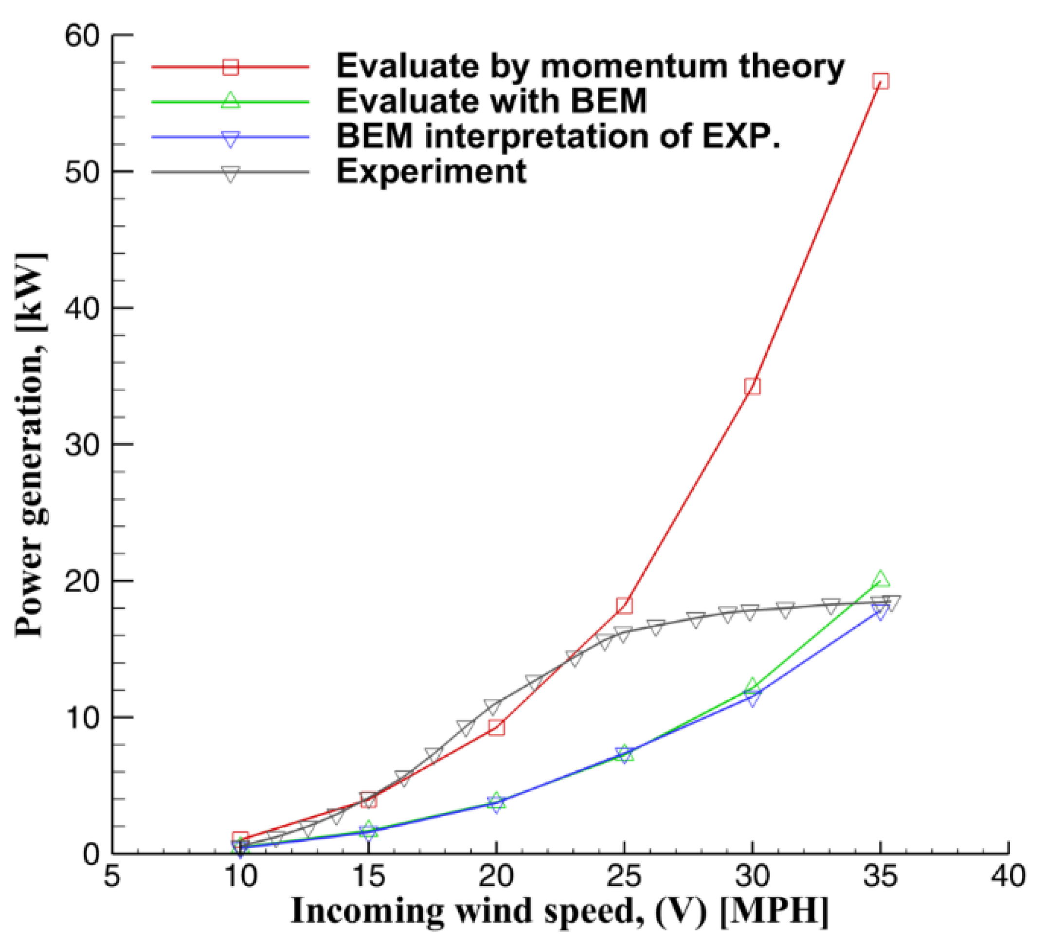
The power generation of a rotor under driving steady wind speed is shown in Figure 7. The gray curve is the measured electric power generation of the Grumman WS33 wind system from Alder, Henton, and King [6]. The angular velocities and angular accelerations obtained from the present simulation data are provided to the momentum analysis theory and BEM method to predict the power generation of the rotor. The red and green curves are the axial power generation of the rotor predicted by the momentum analysis theory and BEM method, respectively. Both of the numerical results were obtained using ANSYS FLUENT 14.
When the rotor operates at a particular angular velocity, which does not make the blade stall, the best performance of the rotor appears. Then, the Q-blade uses this angular velocity to predict power generation of the rotor with the experimental data [6], and the result is shown as the blue curve in Figure 7. The comparison between BEM-calculated results from the ANSYS simulation and Q-blade experiments indicates that the green curve (ANSYS) is very close to the blue one (Q-blade), and the maximum difference between these two curves is below 10% in the higher wind speed range.
Besides, when the driving wind speed is 10 to 25 mph, the predicted power generation difference between the experimental data [6] (gray curve) and the ANSYS simulation data by the momentum analysis theory (red curve) is within 10%. However, the ANSYS simulation data is 2 to 3 times larger than the experimental data [6] when the driving wind speed is 25 to 35 mph.
Since the ANSYS simulation data were obtained without friction on the rotor shaft and the loadings of the gearbox and electric generator, the predictions of power generation by both momentum analysis theory and the BEM method are higher when the driving wind speed is 25 to 35 mph.
In the momentum analysis theory, the wind turbine rotor is assumed as a penetrated static disc, and one can assume uniform pressure distribution on every cross-sectional surface in the control volume. The effects of backflow and vortices in the flow field are both neglected. Therefore, in general, the predictions of the aerodynamic properties of the wind turbine tend to be overestimated by the momentum analysis theory.
When power generation prediction of the rotor is proceeded by the BEM method, the module of the turbulent wake development of the Q-blade is shut down to avoid numerical divergence during the computation processes. Consequently, the forces and torques of the rotor are underestimated if using the BEM method. This underestimation is also coincident with the results of Xu [8].
4. Conclusions
The adaptive dynamic mesh, user-defined functions, and six degrees of freedom solver provided in ANSYS FLUENT 14 were engaged in the present study to simulate the passive rotating process of a rotor transiently without using the combination of conventional MRF and experimentally obtained rotational speed of the rotor to proceed with the CFD simulation as in previous research. The dynamic behaviors and power generation of the rotor attached to the Grumman WS33 wind system during the activating process from a stationary state are shown as a sample task. The rotor was driven by a steady or periodic uniform wind field. The rotational kinematic properties were derived from a post-processed real-time 6DOF solver for the rotor by solving the solid–fluid interactions of the adaptive dynamic meshes. The transient angular velocity and acceleration were calculated directly within the computing processes.
The numerical results reveal that the maximum angular velocity of the rotor is proportional to the mean driving wind speed, and the time to reach the maximal value is inversely proportional to the mean driving wind speed for either steady or periodic wind fields. Besides, the maximal angular acceleration of the rotor is proportional to the square of the mean driving wind speed, and the period of the periodic wind fields does not affect the angular velocity and angular acceleration. The self-similarity property of the evolution process is the first found in numerical simulation studies of wind turbine rotors due to the nearly identical curves about the normalized angular velocities and accelerations presented in the present study.
The power generation of the rotor was predicted by the momentum analysis theory with the present ANSYS simulation data and showed good agreement with experimental data when the driving wind speed was under 25 mph, but was 2 to 3 times larger than the experimental data when the driving wind speed was 25 to 35 mph. The power generation predicted by the BEM method with the ANSYS simulation data and Q-blade data indicates that those two predictions are very close. The results indicated that the simulation methodology proposed is comprehensive and useful. Notably, the present method can predict the transient and passive behaviors of rotor kinematic motions in the design stage of a wind turbine without experimental data.
Author Contributions
Conceptualization, C.-H.H. and J.-L.C.; methodology, C.-H.H., J.-L.C. and K.-Y.K.; software, S.-C.Y.; validation, C.-H.H., J.-L.C. and S.-C.Y.; data curation, C.-H.H. and S.-C.Y.; writing—original draft preparation, C.-H.H. and S.-C.Y.; writing—review and editing, C.-H.H. and J.-L.C. All authors have read and agreed to the published version of the manuscript.
Funding
This research received no external funding.
Conflicts of Interest
The authors declare no conflict of interest.
References
- Betz, A. Introduction to the Theory of Flow Machines; Pergamon: Oxford, UK, 1966. [Google Scholar]
- Hansen, M.O.L. Aerodynamics of Wind Turbines, 3rd ed.; Routledge: New York, NY, USA, 2015. [Google Scholar]
- Hansen, A.C.; Butterfield, C.P. Aerodynamics of horizontal-axis wind turbines. Annu. Rev. Fluid Mech. 1993, 25, 115–149. [Google Scholar] [CrossRef]
- McCroskey, W.J. Some current research in unsteady fluid dynamics. J. Fluids Eng. 1977, 99, 8–38. [Google Scholar] [CrossRef]
- Butterfield, C.P.; Nelsen, E.N. Aerodynamic Testing of a Rotating Wind Turbine Blade; Department of Energy: Morris, MN, USA, 1990.
- Adler, F.M.; Henton, P.; King, P.W. Grumman WS33 Wind System: Prototype Construction and Testing, Phase II Technical Report; Department of Energy, Office of Scientific and Technical Information: Oak Ridge, TN, USA, 1980.
- Huyer, S.A.; Simms, D.; Robinson, M.C. Unsteady aerodynamics associated with a horizontal-axis wind turbine. AIAA J. 1996, 34, 1410–1419. [Google Scholar] [CrossRef]
- Xu, G.; Sankar, L.N. Computational study of horizontal axis wind turbines. J. Sol. Energy Eng. 2000, 122, 35–39. [Google Scholar] [CrossRef]
- Wright, A.K.; Wood, D.H. The starting and low wind speed behavior of a small horizontal axis wind turbine. J. Wind Eng. Ind. Aerodyn. 2004, 92, 1265–1279. [Google Scholar] [CrossRef]
- Silva, C.T.; Donadon, M.V. Unsteady blade element-momentum method including returning wake effects. J. Aerosp. Technol. Manag. 2013, 5, 27–42. [Google Scholar] [CrossRef] [Green Version]
- De Freitas Pinto, R.L.U.; Gonçalves, B.P.F. A revised theoretical analysis of aerodynamic optimization of horizontal-axis wind turbine based on BEM theory. Renew. Energy 2017, 105, 625–636. [Google Scholar] [CrossRef]
- El khchine, Y.; Sriti, M. Tip loss factor effects on aerodynamic performances of horizontal axis wind turbine. Energy Procedia 2017, 118, 136–140. [Google Scholar] [CrossRef]
- ANSYS. ANSYS FLUENT Theory Guide; Release 14.0.; ANSYS Inc.: Canonsburg, PA, USA, 2011. [Google Scholar]
- Gupta, R.; Biswas, A. Computational fluid dynamics analysis of a twisted three-bladed H-Darrieus rotor. J. Renew. Sustain. Energy 2010, 2, 043111. [Google Scholar] [CrossRef]
- Lanzafame, R.; Mauro, S.; Messina, M. Wind turbine CFD modeling using a correlation-based transitional model. Renew. Energy 2013, 52, 31–39. [Google Scholar] [CrossRef]
- Sudhamshu, A.R.; Pandey, M.C.; Sunil, N.; Satish, N.S.; Mugundhan, V.; Velamati, R.K. Numerical study of effect of pitch angle on performance characteristics of a HWAT. Eng. Sci. Technol. Int. J. 2016, 19, 632–641. [Google Scholar]
- Shu, L.; Li, H.; Hu, Q.; Jiang, X.; Qiu, G.; He, G.; Liu, Y. 3D numerical simulation of aerodynamic performance of iced contaminated wind turbine rotor. Cold Reg. Sci. Technol. 2018, 148, 50–62. [Google Scholar] [CrossRef]
- Torregrosa, A.J.; Gil, A.; Quintero, P.; Tiseira, A. Enhanced design of a low power stall regulated wind turbine. BEMT and MRF-RANS combination and comparison with existing designs. J. Wind Eng. Ind. Aerodyn. 2019, 190, 230–244. [Google Scholar] [CrossRef]
- Rodrigues, R.A.; Lengsfeld, C. Development of a computational system to improve wind farm layout, part I: Model validation and near wake analysis. Energies 2019, 12, 940. [Google Scholar] [CrossRef] [Green Version]
- Rodrigues, R.A.; Lengsfeld, C. Development of a computational system to improve wind farm layout, part II: Wind turbine wake interaction. Energies 2019, 12, 1328. [Google Scholar] [CrossRef] [Green Version]
- NREL—NWTC Information Portal. Airfoils Shapes S809. Available online: https://wind.nrel.gov/airfoils/shapes/S809_Shape.html (accessed on 15 November 2020).
- Kondo, J.; Fujinawa, Y.; Naito, G. Wave-induced wind fluctuation over the sea. J. Fluid Mech. 1972, 51, 751–771. [Google Scholar] [CrossRef]
- The Annual Variability of Wind Speed. Wind Energy-The Facts. Available online: https://www.wind-energy-the-facts.org/the-annual-variability-of-wind-speed.html (accessed on 15 November 2020).

Figure 2.
The schematic diagram of the spatial computational domain.

Figure 3.
The mesh element distribution of the computational domain.

Figure 4.
The evolution processes of the angular velocity of the rotor activated from stationary by the various uniform wind fields. (a) Steady wind field; (b) periodic wind field, T = 4 s; (c) periodic wind field, T = 8 s.
Figure 4.
The evolution processes of the angular velocity of the rotor activated from stationary by the various uniform wind fields. (a) Steady wind field; (b) periodic wind field, T = 4 s; (c) periodic wind field, T = 8 s.

Figure 5.
The evolution processes of the angular acceleration of the rotor activated from stationary by the various uniform wind fields. (a) Steady wind field; (b) periodic wind field, T = 4 s; (c) periodic wind field, T = 8 s.
Figure 5.
The evolution processes of the angular acceleration of the rotor activated from stationary by the various uniform wind fields. (a) Steady wind field; (b) periodic wind field, T = 4 s; (c) periodic wind field, T = 8 s.

Figure 6.
The evolution processes of the normalized angular velocity (left column) and angular acceleration (right column) of the rotor activated from stationary position by the various uniform wind fields. (a,b) Steady wind field; (c,d) periodic wind field, T = 4 s; (e,f) periodic wind field, T = 8 s.

Figure 7.
The power generation of a rotor under steady driving wind speed. The experiment curve was plotted using the data of Alder, Henton, and King [6].
Figure 7.
The power generation of a rotor under steady driving wind speed. The experiment curve was plotted using the data of Alder, Henton, and King [6].


Table 1.
The convergence test of the number of mesh elements.
| Elements | 258,951 | 688,523 | 1,619,536 | 8,149,653 |
| Maximal skewness | 0.80337 | 0.84254 | 0.83052 | 0.84366 |
| Relative residuals (0/00) | ||||
| Continuity | 0.891 | 0.911 | 0.956 | 0.997 |
| x-velocity | 8.98 × 10⁻⁵ | 9.16 × 10⁻⁵ | 9.57 × 10⁻⁵ | 9.97 × 10⁻⁵ |
| y-velocity | 8.95 × 10⁻⁵ | 9.25 × 10⁻⁵ | 9.96 × 10⁻⁵ | 9.94 × 10⁻⁵ |
| z-velocity | 5.63 × 10⁻⁵ | 6.79 × 10⁻⁵ | 7.09 × 10⁻⁵ | 6.25 × 10⁻⁵ |
| z-moment | 0.895 | 0.916 | 0.953 | 0.997 |
| Pressure on blade | −1150 | −1150 | −1150 | −1150 |
Table 2.
The ratios between the angular velocities of the rotor driven by steady and periodic wind.
| Mean Wind Speed (mph) | Steady ωs (rad/s) | T = 4 s ωT4 (rad/s) | T = 8 s ωT8 (rad/s) | ωT4/ωs | ωT8/ωs |
|---|---|---|---|---|---|
| 10 | 4.404604 | 5.020789 | 5.018869 | 1.139896 | 1.13946 |
| 15 | 6.582858 | 7.543488 | 7.519751 | 1.145929 | 1.142323 |
| 20 | 8.815134 | 10.06828 | 10.07125 | 1.142159 | 1.142495 |
| 25 | 11.05508 | 12.59643 | 12.59595 | 1.139424 | 1.139381 |
| 30 | 13.25176 | 15.12932 | 15.12460 | 1.141683 | 1.141327 |
| 35 | 15.20250 | 17.35011 | 17.36042 | 1.139951 | 1.141945 |
Table 3.
The ratios between the angular accelerations of the rotor driven by steady and periodic winds.
Table 3.
The ratios between the angular accelerations of the rotor driven by steady and periodic winds.
| Wind Speed (mph) | Steady αs(max) (rad/s2) | T = 4 s αT4(max) (rad/s2) | T = 8 s αT8(max) (rad/s2) | [αT4(max)/αs(max)]1/2 | [αT8(max)/αs(max)]1/2 |
|---|---|---|---|---|---|
| 10 | 0.157080 | 0.202458 | 0.202458 | 1.135292 | 1.135292 |
| 15 | 0.347844 | 0.452215 | 0.452040 | 1.140197 | 1.139977 |
| 20 | 0.618684 | 0.804667 | 0.801001 | 1.140443 | 1.137842 |
| 25 | 0.965691 | 1.251401 | 1.254194 | 1.138359 | 1.139628 |
| 30 | 1.391691 | 1.806416 | 1.855460 | 1.139298 | 1.154661 |
| 35 | 1.883036 | 2.459204 | 2.456725 | 1.142794 | 1.142218 |
Publisher’s Note: MDPI stays neutral with regard to jurisdictional claims in published maps and institutional affiliations. |
© 2021 by the authors. Licensee MDPI, Basel, Switzerland. This article is an open access article distributed under the terms and conditions of the Creative Commons Attribution (CC BY) license (http://creativecommons.org/licenses/by/4.0/).
Share and Cite
MDPI and ACS Style
Hsu, C.-H.; Chen, J.-L.; Yuan, S.-C.; Kung, K.-Y. CFD Simulations on the Rotor Dynamics of a Horizontal Axis Wind Turbine Activated from Stationary. Appl. Mech. 2021, 2, 147-158. https://0-doi-org.brum.beds.ac.uk/10.3390/applmech2010009
AMA Style
Hsu C-H, Chen J-L, Yuan S-C, Kung K-Y. CFD Simulations on the Rotor Dynamics of a Horizontal Axis Wind Turbine Activated from Stationary. Applied Mechanics. 2021; 2(1):147-158. https://0-doi-org.brum.beds.ac.uk/10.3390/applmech2010009
Chicago/Turabian StyleHsu, Cheng-Hsing, Jun-Liang Chen, Shan-Chi Yuan, and Kuang-Yuan Kung. 2021. "CFD Simulations on the Rotor Dynamics of a Horizontal Axis Wind Turbine Activated from Stationary" Applied Mechanics 2, no. 1: 147-158. https://0-doi-org.brum.beds.ac.uk/10.3390/applmech2010009