Comparison of SAFNWC/MSG Satellite Cloud Type with Vaisala CL51 Ceilometer-Detected Cloud Base Layer Using the Sky Condition Algorithm and Vaisala BL-View Software

Abstract

Ceilometer detection can be used to determine cloud type based on cloud layer height. Satellite observations provide images of clouds’ physical properties. During the summer and winter of 2017, Satellite Application Facility on support to Nowcasting/Very Short-Range Forecasting Meteosat Second Generation (SAFNWC/MSG) cloud type was compared to cloud base layers based upon a sky condition algorithm of Vaisala CL51 ceilometer and the BL-View applied range-variant smoothing backscatter profile at the National Atmospheric Observatory in Košetice, Czech Republic. This study investigated whether the larger measurement range of CL51 improved high cloud base detection and the effect of the range-variant smoothing on cloud base detection. The comparison utilized a multi-category contingency table wherein hit rate, false alarm ratio, frequency of bias, and proportion correct were evaluated. The accuracy of low-level and high cloud type detection by satellite was almost identical in both seasons compared to that using the sky condition algorithm. The occurrence of satellite high cloud detection was greatest when the ceilometer detected high cloud base above low and/or medium cloud base. The hit rate of high cloud detection increased significantly when the BL-View-produced cloud base layer was applied as a reference. We conclude that BL-View produces more accurate high cloud base detection.

1. Introduction

Clouds alter the short- and long-wave radiative flux divergence, which in turn modulates the boundary layer dynamics and plays a key role in the problem of climate change. The impact of clouds on solar radiation depends on several factors, such as cloud type, cloud size, and concentration of cloud condensation nuclei. Low clouds predominantly reflect the radiation back to space, while transparent high clouds primarily transmit the incoming solar radiation, trap the emitted long-wave radiation from the surface, and radiate it downward, thereby acting as a greenhouse gas. The cloud types can be observed from the surface by a human observer according to a subjective view of cloud shape and appearance, but several automated ground-based instruments are now available that have been increasingly replacing human-based observations. A pyranometer [1,2], whole-sky infrared cloud-measuring system [3], or hemispherical sky cameras [4,5] define cloud types by radiation measurement. While a ceilometer determines the cloud types by measuring the cloud base height [6,7,8], the radars define the clouds by detecting the cloud top height [6,9].

The Satellite Application Facility on support to Nowcasting/Very Short-Range Forecasting Meteosat Second Generation (SAFNWC/MSG) in cooperation with the European Organisation for the Exploitation of Meteorological Satellites (EUMETSAT) generates, archives, and distributes satellite-derived cloud products (Cloud Mask, Cloud Type, Cloud Top Temperature and Height, Cloud Microphysics) using the characteristics of MSG SEVIRI (Meteosat Second Generation Spinning Enhanced Visible and Infrared Imager) data and of NOAA (National Oceanic and Atmospheric Administration) and EPS AVHRR (EUMETSAT Polar System Advanced Very-High-Resolution Radiometer) data. The cloud type product is derived from satellite radiance measurement with a multispectral thresholding technique [10]. Compared to radar cloud top height detection, according to Karlsson et al. [9], MSG SEVERI is better able to detect the low-level and high-level clouds but has difficulty detecting middle-level clouds. This problem has been largely explained, however, by limitations of the validation method rather than by incorrect assignments of MSG Cloud Types (CTY).

A Vaisala CL51 (Vaisala Oyj, Helsinki, Finland) ceilometer is installed at the National Atmospheric Observatory in Košetice (NAOK) (49.5° N, 15.0° E; Figure 1). Because the CL51 has quite recently been developed, relatively little information is available about its accuracy in cloud layer detection. Liu et al. [11] found that the average cloud occurrence retrieved from the Vaisala CL31 ceilometer was 3.8% greater than that from the CL51 ceilometer. Moreover, in some specific cases, when the Vaisala CL31 ceilometer-detected cloud base height was around 1000 m, the corresponding cloud base height measured by Cl51 was higher. According to Costa-Surós et al. [8], when detecting cloud vertical structure using the CL31 ceilometer, difficulties occurred in retrieving a second cloud layer over a thick first layer. This contributed to an inability to determine the cloud top. Those authors therefore expected that the CL51, with its greater detection range, might improve the cloud base height distribution retrieved.

According to Kotthaus et al. [12], the Vaisala CL31 ceilometer cloud detection depends on the firmware version and whether the instrument is operating in the setting “Message profile noise h2_on” or “Message profile noise h2_off”. Specifications of the Vaisala CL51 at NAOK are detailed in

Table 1. Vaisala CL51 ceilometer specifications for sensor hardware, firmware, message profile noise_h2, time, and range resolution.

Instrument	Ceilometer Engine Board/Transmitter/Receiver	Firmware Version	Profile Noise_h2	Resolution (Time, Range)
CL51	CLE321/CLT521/CLR321	1.32	ON	16 s, 10 m

. Furthermore, the spatial and temporal averaging of the high-resolution attenuated backscatter can increase the signal contribution to the noise. The optimal window length depends on hardware characteristics, resolution settings for raw data acquisition, and the given application [12]. The Vaisala software for boundary layer detection, BL-View, detects the cloud base by a range-variant smoothing window.

In our paper, the Vaisala CL51 ceilometer cloud base height detection by raw and smoothed backscatter profiling was compared with detection using SAFNWC/MSG cloud type data in 2007 winter (DJF) and summer (JJA) periods to answer the following questions:

• Do the high cloud types determined according to SAFNWC Cloud Type data agree with the CL51-detected cloud layer due to the larger range of detection?
• Does the range-variant smoothing window of BL-View improve the cloud base height detection?

The datasets and comparison method are detailed in Section 2. The cloud types determined by SAFNWC/MSG satellite were compared to the cloud types based on cloud layer height retrieved from the Vaisala CL51 ceilometer according to the sky condition algorithm and according to BL-View-produced cloud layers, and these cloud types are analyzed in Section 3. A summary and conclusions are provided in Section 4.

2. Experiments

2.1. Observation

The ceilometer is an essential instrument for detecting the cloud cover and cloud base height based on attenuated aerosol backscatter profile measurement. The Vaisala CL51 ceilometer has a measurement range of 0–15,000 m [13]. The profile enables the user to discriminate cloud from other obstructions (e.g., precipitation) using a fairly straightforward threshold criterion. Its sky condition algorithm provides an observation about cloud amount and cloud layer height at five different layers every 5 min from 16-s measurements based on data collected during the previous 30 min. The last 10 min are double-weighted to make the algorithm more responsive to variations in cloudiness.

The sky condition algorithm contains five modules to calculate the cloud layers and covers from the measured attenuated backscatter. The first is the Initialize module, which selects ceilometer measurements from the last 30 min, sorts them into time order, then distributes them into specific data structures. After that, the module checks whether the ceilometer has provided sufficient data for the algorithm, which is determined by two ratios: the ratio of measurements during the last 30 min, and the ratio of measurements during the last few minutes. If either of these ratios exceeds a threshold value, the data is marked valid and will be used by the rest of the algorithm. If there is no valid ceilometer data, then 99 is returned as sky cover value. If more than 30 min has elapsed, then −1 is returned as sky cover value. Second is the Filter module, which converts ceilometer measurements into cloud hits. If the ceilometer measurement contains multiple cloud bases, the conversion results in multiple cloud hits. The hits are combined into clusters by the Clusterize module. First, this combines the cloud hits into clusters, using an algorithm that looks for layers where the horizontal difference between consecutive hits is small, and then by an algorithm that allows large height differences between consecutive hits. After clustering, a height is assigned for each cluster. First, a height is selected below which 10% of all hits within the cluster are located. The height of the cluster is then calculated as an average of selected hits around this height. After clustering the hits, the Combine module combines clusters into a single list of layers. The module goes through all possible layer heights. A cover value is calculated for each height that is the sum of the cover values of those clusters whose base heights are between the height of the layer and the height of the layer plus the vertical extent of the layer. The vertical extent of the layer is 30.5 m or 10% of the height of the layer. That height with the largest cover value is used in forming a new layer. The height of the new layer is equal to a weighted sum of those clusters that were within the vertical extent of the layer. Finally, the Select module chooses the layers to be reported by the algorithm. The first step is to assign high cloud cover to a single cloud layer. If the highest layer is above the threshold height, then high cloud cover is assigned to that layer; otherwise, a synthetic layer is created at 15,000 m. The second step in the Selected module is to determine which layer to report as being the lowest. After the lowest layer has been determined, the Select module rounds layer heights to 100-foot precision. Layers closer than 100 feet to the layers that are below them or whose sky covers are less than 0.5 octas are combined with the layers that are immediately below them. The height of the combined layer is the height of the lower layer. If the number of layers is still greater than the number of layers requested, the algorithm combines the layer covering the least amount of sky with the layer that is below it [13].

The cloud type detected by the ceilometer can be determined based on cloud layer height, where the low, medium, and high clouds are detected below 2000 m, between 2000 m and 6000 m, and above 6000 m, respectively. The SAFNWC/MSG cloud type algorithm is a threshold algorithm applied at pixel scale based on the SAFNWC/MSG Cloud Mask and spectral and textural features computed from the multispectral satellite images and compared with a set of thresholds [14].

Five cloud type categories were determined based on ceilometer cloud layer height: cloud free (CF), when cloud was not detected in any layer; low cloud (L), if the detected cloud layer was below 2000 m on any cloud layer; medium cloud (M), if the detected cloud layer was between 2000 and 6000 m on the highest cloud layer; high cloud (H), if the cloud layer was above 6000 m in the first cloud layer; and high cloud, above medium and/or low cloud (HaML) if low and/or medium clouds were detected below high cloud. The same categories were defined from satellite data based on the following satellite cloud type (CTY) values: 1 was CF; 5–8 were low cloud; 9–10 were medium cloud; 11–17 were high cloud, because the ceilometer is not able to discriminate semi-transparent and opaque cloud types; and 18 was HaML. A limitation of this comparison is that medium cloud type was defined by the ceilometer even if low semitransparent or fractional cloud layers were detected below medium cloud layers. The motive for this definition was that the satellite view is downward from the top of the atmosphere, and thus its thresholding algorithm is not able to separate low clouds from medium ones.

In this study the ceilometer cloud layer heights were used as reference data, because the ceilometer is more sensitive to clouds than is the satellite instrument.

2.2. Temporal and Spatial Collocations

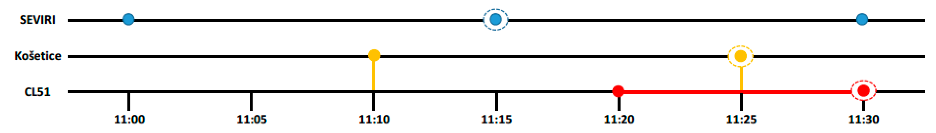
To reach a precise comparison, we applied the time collocation method as detailed by Joro et al. [15]. SEVIRI produces images every 0, 15, 30, and 45 min of each full hour. The instrument scans from east to west and from south to north, and a full disc scan takes roughly 12 min. The remaining 3 min of a scan are used to retract the instrument to the nominal starting position. The Czech Republic is scanned approximately 10 min after the start. Therefore, the nominal repeat cycle (RC) time plus 10 min (RC + 10) was considered to be the real cloud type data acquisition time. We added a 5 min window (RC + 10 + 5) to match the CL51 double-weighted value of the last 10 min. Schematic colocation time is illustrated in Figure 2. For the 11:15 UTC (Coordinated Universal Time) repeat cycle, for example, the real cloud type image acquisition time is taken at 11:25 UTC in Košetice. The ceilometer double-weighted value is received at 11:30 UTC; therefore, we added a 5 min window to search that time.

The spatial collocation was performed by an R script. In this software, the satellite geostationary projection was defined (with proj4 syntax) and the coordinates (latitude and longitude) of NAOK, where the CL51 was installed, were transformed into Geos projection with the spTransform function. From the resulting raster and the particular pixel, we found the SAFNWC CTY values for the CL51 location.

2.3. Comparison

Table 2. Contingency table for comparison of five cloud types based on CL51-detected cloud base layer (in columns) and by SAFNWC/MSG (in rows), where CF is cloud free and HaML is high cloud above medium and/or low clouds. n_i,j are the counts in I = J = 5 events. SAFNWC: Satellite Application Facility on support to Nowcasting; CTY: cloud types.

	CL51-Detected Cloud Base Layer
SAFNWC CTY	CF	Low	Medium	High	HaML	Marginal Sum
CF	n1,1	n1,2	n1,3	n1,4	n1,5	n1
Low	n2,1	n2,2	n2,3	n2,4	n2,5	n2
Medium	n3,1	n3,2	n3,3	n3,4	n3,5	n3
High	n4,1	n4,2	n4,3	n4,4	n4,4	n4
HaML	n5,1	n5,2	n5,3	n5,4	n5,5	n5
Marginal sum	n,1	n,2	n,3	n,4	n,5	N

shows the multi-categorical contingency table used for the comparison.

The counts n_i,j were converted to proportions p_i,j by dividing by the total number of pairs N. The proportion correct (PC) gives the proportion of events where the two observations agree.

$$\mathrm{PC}={\displaystyle \sum }_{\mathrm{i}=1}^5{\mathrm{p}}_{\mathrm{ii}}$$

(1)

The value for perfect agreement is 1 and the poorest value is 0. Frequency bias or just bias (BIAS) represents the ratio of the ceilometer-observed cloud type to the satellite-observed cloud type.

$${\mathrm{BIAS}}_{\mathrm{i}}=\frac{{{\displaystyle \sum }}_{\mathrm{j}=1}^5{\mathrm{p}}_{\mathrm{i},\mathrm{j}}}{{{\displaystyle \sum }}_{\mathrm{j}=1}^5{\mathrm{p}}_{\mathrm{j},\mathrm{i}}}$$

(2)

The perfect value for BIAS is 1. Lower values indicate underestimation, and greater values indicate overestimation of the ceilometer-detected cloud type. The probability of detection (POD), or hit rate, quantifies the success rates of ceilometer-detected cloud type in detecting different categorical events.

$${\mathrm{POD}}_{\mathrm{i}}=\frac{{\mathrm{p}}_{\mathrm{ii}}}{{{\displaystyle \sum }}_{\mathrm{j}=1}^5{\mathrm{p}}_{\mathrm{j},\mathrm{i}}}$$

(3)

The perfect value is 1, the poorest is 0. Only these measures of accuracy are suggested in multi-categorical events according to Joro et al. [15]. The false alarm ratio (FAR) was also taken into account based on Jolliffe et al [16]. FAR is the proportion of cloud types detected only by the ceilometer compared to all ceilometer-observed cloud types in each categorical event.

$${\mathrm{FAR}}_{\mathrm{i}}=\frac{{{\displaystyle \sum }}_{\mathrm{j}=1}^5{\mathrm{p}}_{\mathrm{i},\mathrm{j}}-{\mathrm{p}}_{\mathrm{ii}}}{{{\displaystyle \sum }}_{\mathrm{j}=1}^5{\mathrm{p}}_{\mathrm{i},\mathrm{j}}}$$

(4)

The perfect value is 0 and the worst is 1. The skill scores measure relative skill by comparing the results. Gerrity skill score (GSS) is highly recommended for multi-dimensional contingency tables, because it suits the requirement that multi-categorical forecast misses be scored as poorer forecasts than single-categorical misses.

$$\mathrm{GSS}={\displaystyle \sum }_{\mathrm{i}=1}^5{\displaystyle \sum }_{\mathrm{j}=1}^5{\mathrm{p}}_{\mathrm{i},\mathrm{j}}{\mathrm{s}}_{\mathrm{i},\mathrm{j}}$$

(5)

where s_i,j is a reward (or penalty) array for rewarding correct identification and penalizing the incorrect identification of satellite-detected cloud types. The equations of the weights (s_i,i, s_i,j) are detailed in the Appendix A. The perfect value is 1, while 0 indicates no skill.

3. Results and Discussion

Table 3. Values of proportion correct (PC), frequency bias (BIAS), probability of detection (POD), false alarm ratio (FAR), and Gerrity skill score (GSS) in winter (DJF) and summer (JJA) when SAFNWC/MSG was compared to the Vaisala CL51 sky condition algorithm-detected cloud layers.

	DJF					JJA
	CF	L	M	H	HaML	CF	L	M	H	HaML
PC	0.57					0.48
BIAS	1.50	0.56	0.97	4.08	0.93	1.56	0.87	0.28	1.89	0.68
POD	0.96	0.53	0.22	0.54	0.02	0.63	0.45	0.19	0.45	0.06
FAR	0.35	0.04	0.77	0.86	0.98	0.83	0.47	0.30	0.76	0.91
GSS	0.43					0.37

shows the values for PC, bias, POD, and FAR in the winter and summer periods while considering the sky condition algorithm-produced cloud layer heights. There was no significant difference between the results in the two seasons. According to the POD results, the SAFNWC/MSG could detect the low and high clouds with the same accuracy comparing the ceilometer data. The poor agreement in the HaML category—POD of 0.02 and 0.06 in winter and in summer, respectively—shows that SAFNWC/MSG had a weakness in separating low- or middle-level clouds from high clouds. The disagreement regarding medium-level clouds can be explained by the different geometrical observations. The ceilometer detected the cloud base upward from the surface, while the satellite viewed downward from the top of the atmosphere. Medium cloud types detected by ceilometer could be observed by satellite in the upper part of the medium cloud layer. In addition, the vertically developing clouds (e.g., cumulonimbus), the base of which occurred in the middle level and top in the high level, could be observed.

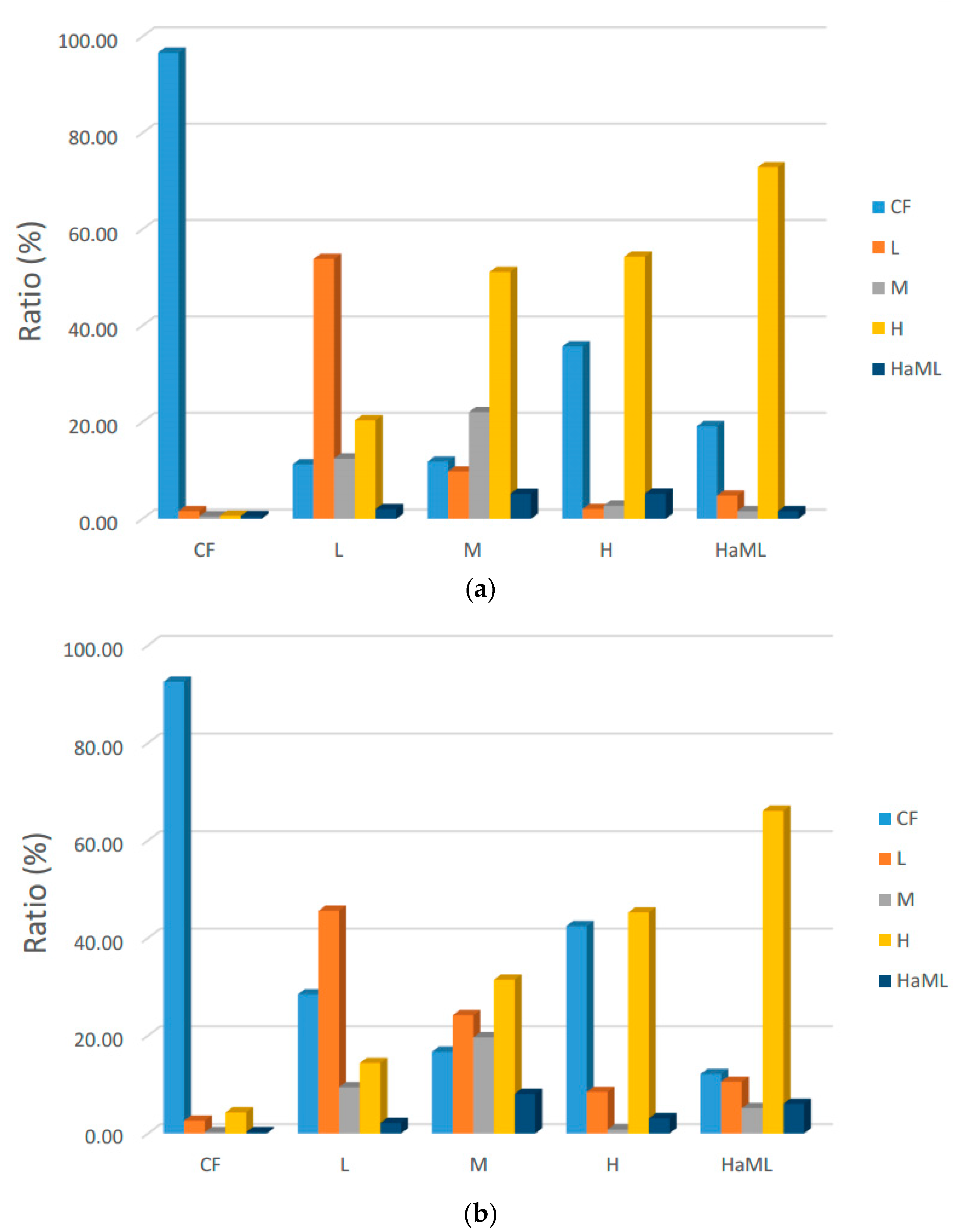
Figure 3a,b shows the ratio of occurrence of SAFNWC-detected cloud types in the cloud type categories according to the Vaisala CL51 sky condition algorithm-detected cloud base height. The ratio was calculated by the following equation:

$$R_i= \frac{p_{i,j}}{{{\displaystyle \sum }}_{j=1}^5{p}_{j,i}}$$

(6)

It shows the POD values if the two instruments detected the same cloud type.

Good agreement can be seen in the cloud-free category. The low-level cloud detection of the satellite had 53% agreement with the ceilometer, and the other cloud type occurrence was less than 20% in winter (Figure 3a). In summer, the satellite-detected cloud-free category increased to 28% when the ceilometer detected low-level clouds (Figure 3b). When the ceilometer measured high cloud base layers, the satellite detected mainly high (54%, 45%) clouds or did not detect cloud (36%, 42%) in winter and summer, respectively. When the ceilometer measured the high cloud layer above low- and/or medium-level cloud layers, the satellite detected dominantly high clouds (73%) in winter and in summer (66%). The other detected cloud types were less than 20% in the HaML category. On one hand, this result points to the fact that the satellite cannot correctly detect multi-layer clouds, while, on the other hand, there is good agreement between the two instruments in detecting high clouds.

Table 4. Values of PC, BIAS, POD, FAR values, and GSS skill score in DJF and JJA periods when SAFNWC/MSG was compared to BL-View-detected cloud layers based on range-variant smoothing of Vaisala CL51 aerosol backscatter profile.

	DJF					JJA
	CF	L	M	H	HaML	CF	L	M	H	HaML
PC	0.60					0.57
BIAS	1.17	0.57	1.11	4.86	17.6	0.92	1.12	0.36	3.34	7.46
POD	0.89	0.53	0.24	0.72	0.00	0.77	0.49	0.23	0.63	0.09
FAR	0.24	0.06	0.78	0.85	1.00	0.15	0.56	0.34	0.72	0.98
GSS	0.46					0.41

demonstrates the PC, BIAS, POD, FAR, and GS values in the case of comparing SAFNWC cloud type with BL-View software-produced cloud base layer heights based on range-variant smoothing of the aerosol backscatter profile.

The range-variant smoothing of the backscatter profile increased the PC values in both seasons. Significant improvement was found in high cloud detection, where the POD value changed from 0.54 to 0.72 in winter and from 0.45 to 0.63 in summer. The FAR values changed rather little, however.

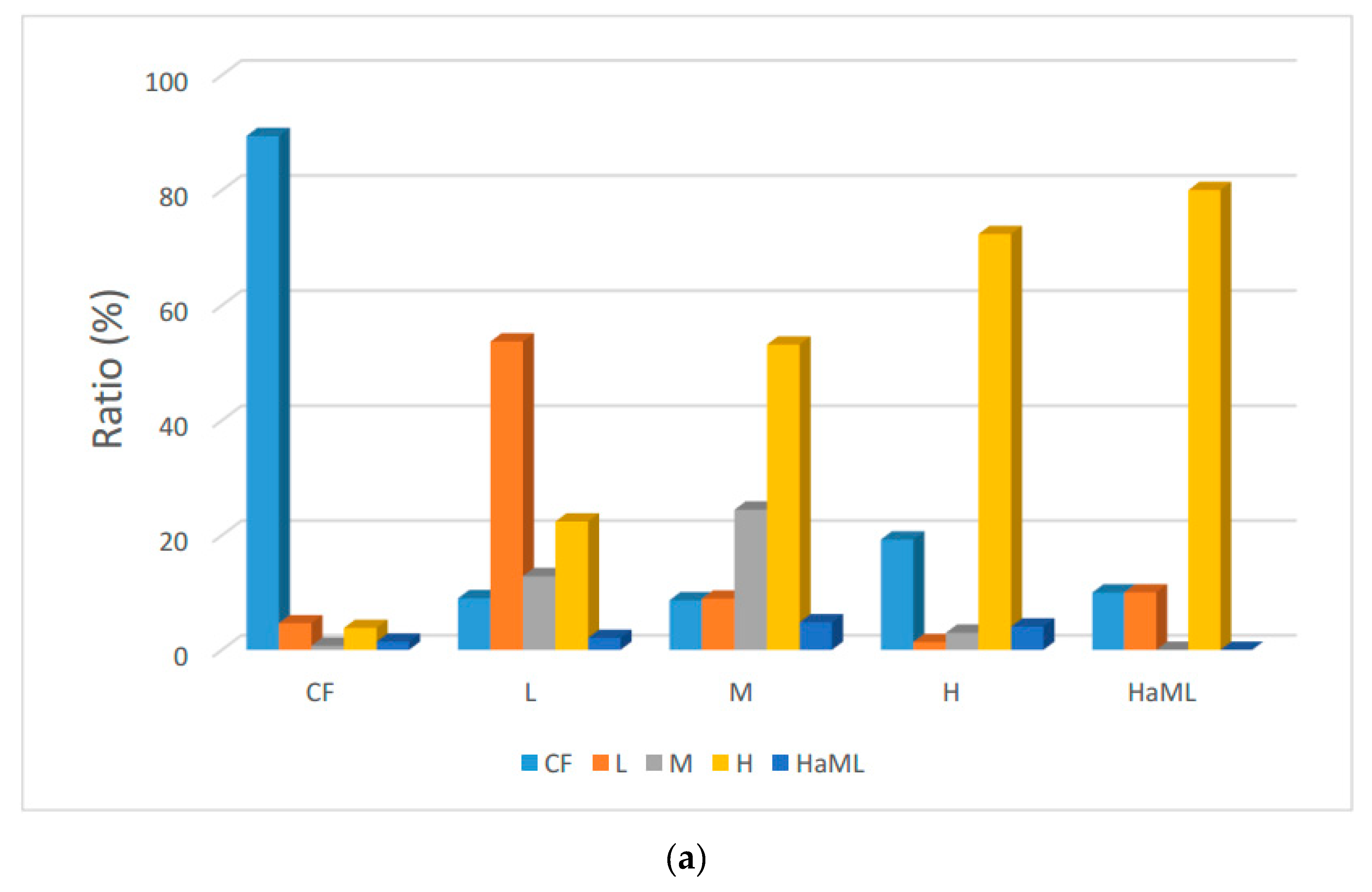
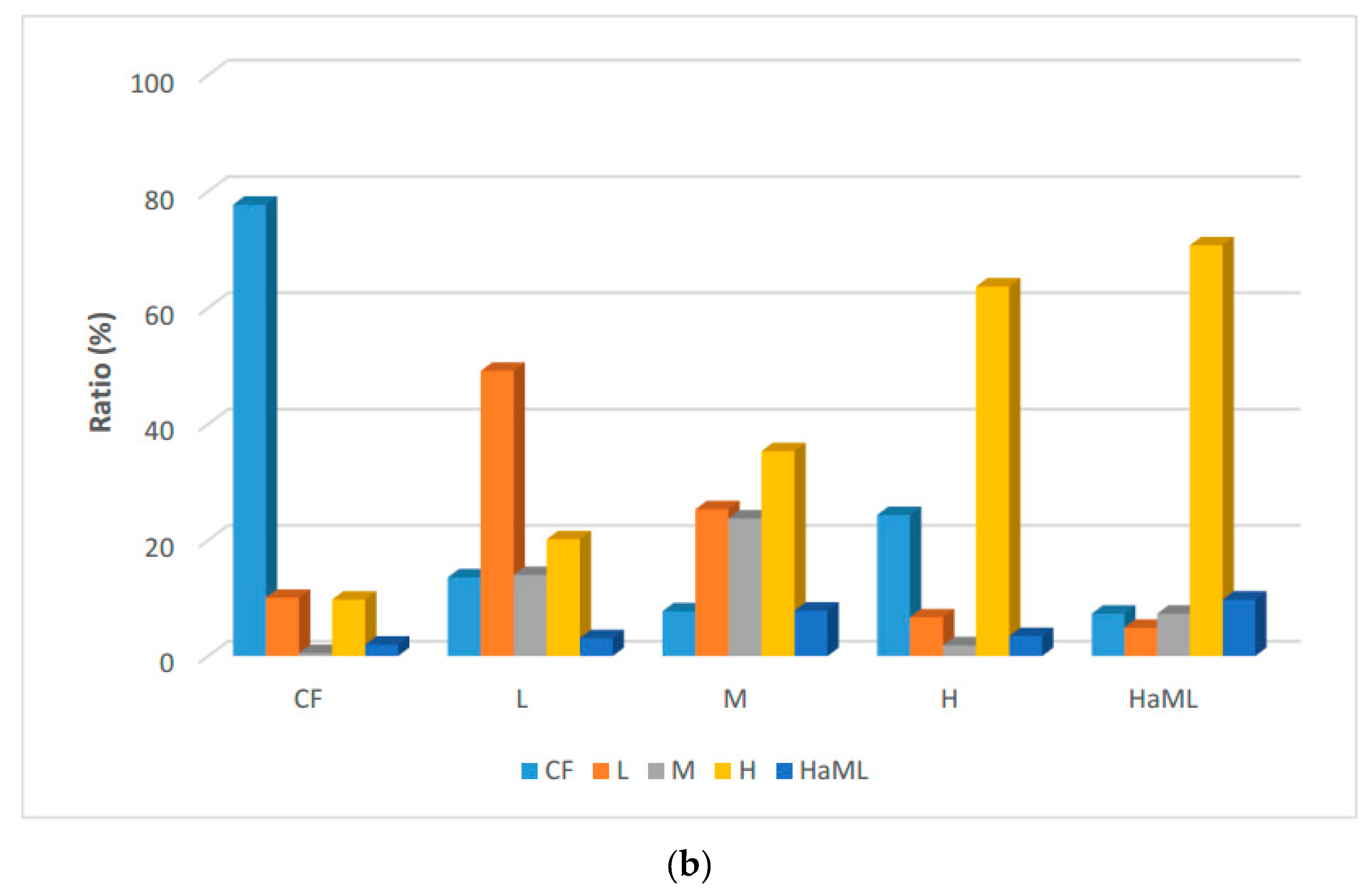
Figure 4a,b shows the occurrence of SAFNWC cloud types in cloud type categories according to BL-View-detected cloud layer heights. Compared to Figure 3 and Figure 4, a significant difference can be seen in the high cloud category, where the agreement increased and the satellite CF ratio decreased. Moreover, the satellite high cloud ratio increased in the HaML category, where the ratio was 80% in winter (Figure 4a) and 71% in summer (Figure 4b).

4. Conclusions

SAFNWC/MSG satellite cloud type detection was compared with the cloud base layers of the Vaisala CL51 sky condition algorithm and with the BL-View-detected cloud layers by range-variant smoothing of the Vaisala CL51 backscatter profile in the 2017 winter and summer periods. Our purpose was to investigate whether the SAFNWC high cloud type agreed with the CL51 high cloud layer detection due to the larger range detection, and if the range-variant smoothing of the backscatter profile improved high cloud layer detection. The low-level, medium-level, and high-level clouds were defined based on cloud base layer height. In addition, we compared the multi-layer cloud detection when high clouds were observed above low and/or medium cloud layers. Although ceilometer measurements were used as the reference data, if the satellite-detected high cloud type agreed with the ceilometer high cloud base layer, we concluded that the CL51 was improved in relation to high cloud detection, because the satellite instrument is sensitive to high clouds.

The hit rate in low-level and high cloud types was almost the same in the two seasons when the comparison was made using the sky condition algorithm. In the case of the medium-level cloud comparison, we cannot draw a conclusion due to the different methods of cloud detection. As shown by the comparison with the ceilometer data, SAFNWC has a limitation in its ability to detect medium or low clouds below the high clouds. The satellite detected mainly high cloud types, while the ceilometer detected high cloud layers above low- and/or medium-level clouds. We can conclude from this result that the larger range detection did improve the high cloud detection of the ceilometer. We also found that the range-variant smoothing of the backscatter profile significantly improved the high cloud layer detection.