Study of Realistic Urban Boundary Layer Turbulence with High-Resolution Large-Eddy Simulation


1
Atmospheric Dispersion Modelling, Atmospheric Composition Research, Finnish Meteorological Institute, 00560 Helsinki, Finland
2
Institute of Atmospheric and Earth System Research, Faculty of Science, University of Helsinki, 00560 Helsinki, Finland
3
Department of Mathematics and Statistics, University of Helsinki, 00560 Helsinki, Finland
4
OP Financial Group, 00510 Helsinki, Finland
5
Department of Forest Sciences, University of Helsinki, 00790 Helsinki, Finland
6
Helsinki Institute of Sustainability Science, University of Helsinki, 00014 Helsinki, Finland
*
Author to whom correspondence should be addressed.
†
Current address: Erik Palménin Aukio 1, 00560 Helsinki, Finland.
Atmosphere 2020, 11(2), 201; https://0-doi-org.brum.beds.ac.uk/10.3390/atmos11020201
Submission received: 30 December 2019
/
Revised: 27 January 2020
/
Accepted: 5 February 2020
/
Published: 13 February 2020
(This article belongs to the Section Atmospheric Techniques, Instruments, and Modeling)
Abstract
:This study examines the statistical predictability of local wind conditions in a real urban environment under realistic atmospheric boundary layer conditions by means of Large-Eddy Simulation (LES). The computational domain features a highly detailed description of a densely built coastal downtown area, which includes vegetation. A multi-scale nested LES modelling approach is utilized to achieve a setup where a fully developed boundary layer flow, which is also allowed to form and evolve very large-scale turbulent motions, becomes incident with the urban surface. Under these nonideal conditions, the local scale predictability and result sensitivity to central modelling choices are scrutinized via comparative techniques. Joint time–frequency analysis with wavelets is exploited to aid targeted filtering of the problematic large-scale motions, while concepts of information entropy and divergence are exploited to perform a deep probing comparison of local urban canopy turbulence signals. The study demonstrates the utility of wavelet analysis and information theory in urban turbulence research while emphasizing the importance of grid resolution when local scale predictability, particularly close to the pedestrian level, is sought. In densely built urban environments, the level of detail of vegetation drag modelling description is deemed most significant in the immediate vicinity of the trees.
1. Introduction
In a rapidly urbanizing world, it is important to improve our understanding of the turbulent dispersion and exchange processes influencing the microclimate and air quality of our cities. This poses a challenge because urban boundary layer (UBL) flows are complex flow systems that arise from the interaction between atmospheric boundary layer (ABL) turbulence and varying arrangements of urban obstacles [1]. While the general urban layout, characterized by the mean building (or building block) height, density, and orientation, governs the wind dynamics in a statistical sense, the actual aerodynamic properties of individual obstacles dictate the local flow conditions which bear the greatest significance to people residing or working in the area. Thus, it is important to aquire the ability to predict these local scale flow system details for they strongly influence the local exchange rates of momentum, heat, and humidity, as well as the dispersion rates of pollutants [2,3,4,5].
Real cities have complicated morphologies due to the inherent variability in the shape and size of urban roughness elements (e.g., buildings, building blocks, individual street trees, and patches of park trees), and the frail appearance of topographic regularity is typically broken by the presence of openings (e.g., lawns, market places, and parking lots) that can significantly alter the local wind conditions. Parameterized approaches to UBL flows (e.g., References [6,7]) do not provide the means to identify and examine such complex, real world urban configurations in a targeted fashion. Only high-fidelity numerical or experimental techniques capable of capturing the relevant flow processes despite the complexity can offer a sufficiently accurate mechanism to study these flow systems. Unfortunately, the study of real urban climate is hindered by the difficulty and cost associated with performing thorough measurement campaigns in the field or in the wind tunnel. Luckily, the latest numerical modelling techniques, computational resources, and remote scanning datasets do offer tantalizing opportunities to examine realistic urban flow schenarios with models that describe the urban surface with an ever increasing level of detail. Particularly Large-Eddy Simulation (LES), a modelling approach in the field of Computational Fluid Dynamics (CFD) capable of temporally and spatially resolving the relevant turbulent processes governing the transport and exchange of momentum, energy, and materials between the urban surface and the ambient air, provides a well-established modelling framework with which the relevant turbulent processes in complex UBL flows can be simulated [8,9].
The research on UBL turbulence has progressed through an incremental course which initially, justifiably, exploited parametrized urban surfaces described by an arrangement of regular cuboids. The ability to resolve idealized urban canopy flows with the LES technique has been demonstrated via a series of studies involving comparisons with wind tunnel and direct numerical simulation (DNS) results [10,11,12,13,14,15,16,17,18,19], establishing the complex nature of fundamental urban canopy turbulence, its weak dependency on Reynolds number (at realistic, high Re conditions), the flow solutions’ relative indifference to the choice of subgrid scale (SGS) turbulence model, and the general LES resolution requirements for capturing the relevant flow physics between and above regular urban roughness elements. The view on UBL flows is further augmented by a series of studies featuring real urban neighborhoods [2,3,4,5], providing additional quantification on the flow behavior and turbulent transport mechanisms within the roughness sublayer (RSL), the vertical range of the UBL within which the effect of individual urban obstacles are observed. These works employed rather restricted ABL turbulence, featured limited urban domains, and excluded urban vegetation. Urban vegetation plays an important role in UBL flows, explicated by Giometto et al. [20] in an LES study featuring a suburban setting. Furthermore, the validation study featuring real urban complexity (but without trees) documented in References [21,22] provides a relevant account of validation approaches, some of which are adopted and expanded upon in this work. Unfortunately, the resolution of their LES model was clearly insufficient to demonstrate the full capacity of LES in urban flow problems.
While the arbitrary complexity of real urban environments demands a high degree of accuracy from the LES simulations, it also brings to focus a central question concerning the necessary level of detail of the model inputs. Thus, considering the difficult nature of real urban flows, we must ask what is the meaningful level of detail with which the urban roughness elements, buildings, and particularly vegetation must be described within the model? This study examines issues relating to local scale predictability and the observability of changes in realistic UBL flows where the situation is further complicated by nonideal conditions. For instance, many major cities are situated near the coastline, which causes the boundary layer flow to abruptly go though a transition from smooth surface to rough surface flow (or vice-versa) as the wind crosses the shoreline. These transitions disturb the flow and create significantly large areas where developing boundary layer flow conditions prevail. Also, in real UBL flows, where the urban roughness interacts with real ABL turbulence, the divide between the smallest and the largest turbulent scales becomes particularly pronounced. Even under near neutral ABL conditions (most suitable for validation efforts) the flow contains both large-scale and very large-scale turbulence motions (LSM and VLSM) of which the time scales are so long that it is unreasonable to expect local in situ measured time series to capture sufficiently converged statistics on them. Therefore, it is necessary to examine the complexities real urban flows impose and to seek methodologies to extract relevant information even concerning the local scale processes.
This numerical study employs state-of-the-art LES modelling techniques to examine a realistic UBL flow scenario designed to bear close correspondence with observable urban turbulence under neutral stratification. The PArallel Large-eddy Simulation Model (PALM) LES solver [23], with a newly added nested multi-scale system [24], is used to perform numerical simulations. The LES model domain features a highly detailed description of downtown Helsinki, a coastal capital city of Finland accommodating a variety of urban microclimate studies [25]. The considered city domain contains a significant amount of urban vegetation, which is included in the LES model as porous media. The study transparently documents the employed model configuration where fully developed ABL turbulence becomes incident with the urban surface, generating a developing UBL flow characteristic for coastal cities.
The numerical setup is designed to allow the ABL flow to develop and evolve very large-scale streamwise structures that are observed in high Reynolds number boundary layer flows (see e.g., Hutchins et al. [26], Fang and Porté-Agel [27], and references therein). These very large-scale motions (VLSM) of ABL, of which the length scales extend well beyond the boundary layer height , introduce difficulties in analyzing real urban turbulence statistics as the diurnally changing ambient conditions impose limits on the considered time series length. Thus, this work deliberately adopts a confined approach, where the considered time series do not yield sufficiently converged statistics on the VLSMs, and examines the sensitivity of the urban LES solution to central numerical modelling choices via comparative techniques. Particular emphasis is placed on the aerodynamic modelling of urban vegetation due to the embedded uncertainties in determining their spatial extent and aerodynamic attributes. The sensitivity of LES-resolved UBL turbulence to the alterations in vegetation model is examined in juxtaposition to its sensitivity to the modelled height of the ABL. This aspect is considered because the considered UBL flow is developing, having gone though a sharp transition at the leading edge of the city as the ABL flow becomes incident with the shoreline. Here, the inference that, under fully developed UBL conditions, the low altitude RSL turbulence is insensitive to outer layer dynamics is considered insecure, warranting confirmation in the chosen context. In addition, the considered sensitivities in local turbulence signals are also compared against the effects arising from an elementary reduction in grid resolution.
The comparative post-processing analysis starts by evaluating deviations in two-dimensional mean flow distributions over horizontal planes and proceeds by comparing the contents of virtual tower measurements extracted at different locations within the downtown area. The local tower measurements are subjected to joint time–frequency analysis with wavelets to inspect the makeup of the simulated turbulent fluctuations with some level of temporal coherence across different frequencies (or scales). In an effort to expose deviations in the local turbulent signals that arise due to the model modifications, concepts of information entropy and divergence are exploited in conjuction with wavelet analysis to carry out a deep probing comparison of LES-resolved urban canopy turbulence. These mathematical techniques are robustly introduced to establish a solid foundation for their utility in UBL turbulence research.
Due to the high degree of complexity of the UBL turbulence, this study aims to address what is the required level of detail for the urban surface description within high-resolution LES models. This information is relevant considering that the highest quality (vegetation resolving) light detection and ranging (LiDAR) scan datasets are not publically available for many potential study sites. This work is also considered a relevant precursor for future validation efforts, providing guidelines for the urban LES modeling and further identifying the bounds within which agreement against urban in situ measurements can be sought considering the modelling uncertainties and observation limitations.
2. Materials and Methods
2.1. Note on Nomenclature
Throughout this document, Cartesian vectors are denoted by boldface font and scalars are denoted by normal font. Thus, for instance, the coordinate vector and its components are denoted as . In the context of LES, the velocity vector obeys the following decomposition , where is the unfiltered velocity field, is the space filtered (grid resolved) velocity, and is the subgrid-scale velocity. The Cartesian velocity vector components are , whereas the flow components in a horizontally rotated coordinate system , where the -axis is aligned with the mean flow’s streamwise direction, are marked as , where is the component in the mean streamwise direction, is the component in the mean crosswind direction, and is the vertical component. These velocity components are computed as follows:
where is the local horizontal mean flow direction. The Reynolds decomposition of the resolved velocity field follows the convention , using overbar to indicate a temporal average and prime to specify fluctuations about the mean. By default, angled brackets denote a horizontal average, while a subscript is used in other situations. All the spatial averages in this text are intrinsic averages (see Whitaker [28], Schmid et al. [29]), where all data points representing air or porous media (vegetation) are included while points within solid obstancles are excluded.
2.2. Large-Eddy Simulation Solver PALM
In this study PALM [23] LES model is utilized to study developing urban boundary layer flows. The solver employs finite-difference discretization on staggered Cartesian grid to numerically integrate the filtered, Boussinesq-approximated Navier–Stokes equations for incompressible flows, presented here using vector notation while omitting moisture- and Coriolis acceleration-related terms as they are not relevant in this study:
In Equation (2), g is the gravitational accelaration, is the unit vector in the z direction, is the identity matrix, is the subgrid-scale kinematic stress tensor as ⊗ denotes the outer vector product, is the modified perturbation pressure ( being the perturbation pressure), and is the constant density of air at ground level. In the energy equation, Equation (3), is the potential temperature and is the subgrid scale temperature flux vector.
PALM solves the governing equations on a regular hexagonal domain with a boundary , where the boundary set consists of , which refer to the left, right, north, south, top, and bottom boundaries of the domain. The superscript n is the identification label of the domain, which is relevant when multiple domains are coupled via nesting technique (see Section 2.2.1 below).
For the discretization of the advection and diffusion schemes, the fifth-order Wicker–Skamarock and second-order central difference schemes are employed, respectively [30]. The solution strategy of PALM is based on a 3rd-order accurate Runge–Kutta time-stepping scheme and a predictor-corrector approach, where the divergence generated by the predictor step in the velocity field is subsequently removed by a corrector step utilizing the solution to a Poisson equation for . An efficient iterative multigrid solver is used for the pressure solution. To attain closure in the final system of filtered equations, PALM implements the 1.5-order subgrid-scale (SGS) turbulence model by Deardorff [31] with modifications due to Moeng and Wyngaard [32] and Saiki et al. [33].
The PALM model system includes also a newly implemented surface energy model [34], which incorporates the principal surface energy budget processes occurring within urban environments. Since the objective of this study is to examine the impact of certain modelling choices and their observability in an urban flow system under neutral ABL conditions (when only the anthropogenic heat component is relevant), the functionality of the USM is not exploited here.
2.2.1. Nested LES Domain Approach
The PALM solver has been recently implemented with a self-nested domain approach, which allows multiple solution domains with decreasing domain sizes but increasing resolutions to be solved simultaneously in a coupled manner. This approach facilitates an efficient simulation of flow problems that contain a wide range of turbulent scales by making it possible to employ higher resolution only where necessary. In this context, a notational convention is adopted for labeling domains, where the superscript includes a unique identifier n for every so-called child domain and an optional parent entry to indicate whether domain n has a parent domain p within which it is fully contained. In situations where parent information is not critical, shorter notation may be used. By convention, the main parent domain (which defines the outer boundaries of the LES model) is denoted , whereas the subsequent child domains become , noting that always applies. The boundary notation is also adjusted accordingly such that, for instance, refers to the top boundary of domain .
The solutions of each parent and child pair are coupled either by one-way or two-way coupling schemes (see Hellsten et al. [24] for details). In this study, the LES model is composed of three one-way coupled domains forming a nested system . Table 1 lays out the relevant information on each computational domain. In the one-way coupling scheme, the parent domains provide time-accurate Dirichlet boundary conditions for every prognostic variable on , excluding the bottom boundaries where identical solid wall boundary conditions are employed on all domains. The one-way coupling scheme is particularly well suited for the considered advection-driven UBL flow study where it is desired that the solution of the coarser domains remain unaltered by the finer nested domain solutions (which is contrary in the two-way coupling mode.) The boundary conditions are further described in Section 2.4.1.
2.3. Urban Surface Model in LES
This study utilizes a numerical model that features a detailed description of a real urban area (Figure 1). The surface model features a area of downtown Helsinki, the coastal capital of Finland. This region contains a dense arrangement of perimeter blocks, an irregular distribution of vegetated openings and streets (boulevards), and a network of narrow street canyons plus a central multilane artery that divides two downtown districts. The chosen area encompasses universal elements of low built urban environments that are common particularly within European cities. The urban surface model is constructed from an open access LiDAR dataset (accessible via http://hel.fi/3D) provided by the City of Helsinki. For the purpose of this and future urban LES studies, the point cloud dataset has been processed to yield a series of detailed raster maps, including topography (i.e., digital elevation model (DEM)), orography (land surface elevation), vegetation height, and land cover distributions. These raster materials are also made openly accessible for the community [35].
Information concerning the surface morphometry of the and model domains is presented in Table 2. The relevant mean canopy height is assigned m, which very closely matches the mean building height of the domain and the upwind sector belonging to . The plan and frontal area fractions of obstacles are defined as and , where is the planar area of obstacles at ground level, is the total frontal area (visible to the flow) of obstacles, and is the total planar area of the domain. Using the flow regime categorization for idealized urban canopies according to Hussain and Lee [36], the obtained building area fractions classify the urban area as dense where skimming flow dominates [37]. However, due to the irregularity in building morphologies and variability in street canyon orientations and vegetation distributions, such flow regime characterization offers little information about the considered urban canopy flow.
The building and tree height distributions in Figure 2 illustrate the symmetric variability in building heights (except for the single outlier at ) and the positive skew distribution of the vegetation heights. The vegetation height distribution closely resembles that of a suburban area reported by Giometto et al. [20], except that here the small plants and shrubs with m are not explicitly described by the dataset. The effect of the low vegetation and other fine structural details (balconies, small chimneys, roof ventilator, etc.) are taken into account via surface roughness parametrization in the LES simulation (see Section 2.4 below).
2.4. LES Modelling
To facilitate this comparative investigation of local scale urban canopy turbulence, a baseline LES simulation setup is established to act as a reference onto which each individual alteration is subsequently introduced. The wind direction is held unaltered for the all the simulations because the structural complexity and irregular orientation of the considered city plan introduces a significant amount of directional and structural variation into the roughness sublayer turbulence.
2.4.1. Boundary Conditions and Initialization
The inlet boundary condition on is designed to represent fully developed neutral ABL turbulence, which contains the appropriate range of length scales and remains unaffected by the urban roughness. This is achieved by employing the turbulence recycling technique (see References [23,38] for details), where the inlet boundary value is constructed from two contributions
Here, is any prognostic variable such that the predetermined mean vertical inlet profile is held fixed while the fluctuating components are recycled to the inlet from a specified recycling plane at downstream (drawn in Figure 1). Only the fluctuations occuring for are recycled, and therefore, is utilized as the boundary layer height for the reference case from here on. The recycling height is modified in one of the documented simulations.
The inlet profiles for the prognostic variables are generated by precomputing a fully developed ABL solution, called a precursor solution, on a domain outlined in the bottom left corner of Figure 1, with periodic lateral boundary conditions and no-slip and free-slip conditions at the bottom and top, respectively. This flow is driven by a prescribed negative pressure gradient, which is imposed for . The magnitude and direction of the pressure gradient is adjusted such that and the flow angle with respect to the x-axis is . The recycling method yields a flow solution, in which the double-averaged profiles in Figure 3 closely resemble ABL flow in geostrofic balance, featuring a constant momentum flux layer at . However, this setup exhibits faster convergence. The precursor simulation was initialized with a guessed mean profile and computed for , as , to obtain well-converged double-averaged profiles from the last .
The flow field of the urban LES simulation is, in turn, initialized by repetitively copying the precursor flow solution to the domain. The prognostic variables within the and domains are initialized by interpolating the parent domain values onto their respective grids.
The relatively long frontal section representing ABL flow over sea surface is constructed to facilitate the development and evolution of large-scale and very-large-scale motions, termed LSM and VLSM, respectively, that are observed in pipe, channel, and boundary layer flows (see, for example, References [26,39,40,41,42], and references therein). The presence and relevance of these long streamwise structures, which affect the low altitude roughness sublayer flow via amplitude modulation, have been thoroughly established [43,44,45,46] in near neutral ABL flows, implying they ought to be considered a universal trait of UBL flows under similar conditions. Therefore, despite the statistical convergence difficulties they introduce, the inclusion of the large-scale boundary layer motions is deemed essential in the presented simulations as close compatibility is sought between modelled and (in the future) measured urban turbulence.
The small flow angle in the simulated ABL flow is important because the turbulence recycling setup is prone to numerically amplifying the elongated streamwise disturbances, causing the VLSM flow between the recycling planes to become correlated with the inlet [47]. The small -component forces the LSM and VLSM structures to traverse the domain in the spanwise direction and to evolve without numerical amplification. This requires the distance between the inlet and the recycling plane to be sufficiently long. For this configuration, the distance is found to be adequate when the mean flow angle results in displacement in the lateral direction as the flow moves from the inlet to the recycling plane.
The placement of the recycling plane is also sensitive to the disturbances that travel upstream from the leading edge of the urban surface. In this study, the disturbances generated by the real, unsymmetric shoreline of Helsinki gives rise to a weak perturbation at the recycling plane, which is subsequently transported all the way to the inlet. This perturbation manifests by adding a weak but observable systematic stripiness in the mean flow. This influence could be eliminated by substantially increasing the distance between the recycling plane and the leading edge of the city. However, a computationally more efficient technique is utilized here instead. The effect of the unsymmetric disturbances is diminished by adding a single sparse array of narrow but tall spires ( wide “towers” reaching a height , placed apart) right after the inlet plane. These structures introduce a minor but regular source of small-scale disturbances that do not have an observable impact on the generated ABL flow far downstream but make the turbulence recycling boundary conditions more immune to amplification of upwind travelling disturbances from the urban roughness.
In each computational domain, the no-slip wall boundary condition is imposed for all , including the building walls. The shear stress at the wall is computed in accordance to the logarithmic law of the wall with roughness, taking into account the effect of the roughness elements not resolved by the computational grid by assigning the subgrid-scale aerodynamic roughness length . The thermal landscape of the city due to anthropogenic sources is taken into account in a simplified manner by assigning a Dirichlet condition , where is the constant potential temperature of air from the neutral precursor simulation and is the urban surface. The inclusion of anthropogenic heat is not relevant for this comparative study, but it is deemed an inherent ingredient of UBL flows under neutrally stratified atmospheric conditions.
2.4.2. Modeling of Trees as Porous Media
The difficulty of including trees within an urban LES model originates from the complex nature of their aerodynamic impact. The drag caused by an individual tree is much higher when it is isolated compared to being part of a forest canopy where the trees shelter each other. The earlier fundamental research on the effects of vegetation in ABL flows has considered continuous canopies where individual trees or vegetation elements are not identifiable objects with distinct spatial and aerodynamic properties or such that the canopy is constructed from a regular array of distict objects; see e.g., References [48,49,50,51,52].
Within densely built urban environments, the situation is complicated by the sporadic appearance of vegetation. Trees are typically planted individually along boulevards, esplanads, and other roads, whereas parks and other green areas may feature clusters of trees where the merging of foliage may form canopy-like patches. LiDAR measurements can provide spatially resolved information on the structural density of tree foliage, but their point cloud datasets may not provide reliable information concerning the inner structure of trees that have large crown sizes and dense leaf covers. The quality of this data depends on the amount of LiDAR beam reflections obtained from the inner part of the foliage. Even in the case of accurate structural probing of trees, their location with respect to the wind and each other strongly influence the aerodynamic properties they possess. For this reason, the modelling of vegetation within urban environments carries significant uncertainties of which the overall impact on the urban flow system needs to be established before detailed air quality and urban plan investigations featuring real urban sites can be undertaken.
In the PALM LES model, the aerodynamic drag due to vegetation is modelled as a momentum sink in the form of pressure drag (assuming the viscous drag contribution to be negligible in comparison) and is formulated as follows:
where is a constant drag coefficient for vegetation and is the leaf area density or, synonymously, plant area density of discretized tree elements (cells in the grid occupied by foliage). The is the ratio of the plant’s surface area (visible to the flow) to the volume it occupies. In this study, the uncertainty in the effective drag coefficient which combines the two model inputs is scrutinized by imposing variations in both and that are expected to span a relevant fraction of the uncertainty range associated with these inputs.
The formulation of Equation (4) simplifies a complex problem by splitting the user specified elements of into a universal constant and a plant’s density measure, which is solely determined by the spatial attributes of the tree. This is immediately problematic because trees are not only spatially complex objects but also elastic structures of which the structural and aerodynamic properties (e.g., branch rigidity, leaf, or needle shape reconfiguration under wind loads) can vastly vary between different species. Experimental drag coefficient measurements carried out by, for example, Mayhead [53], Rudnicki et al. [54], and Vollsinger et al. [55], reveal the wide scatter of result between different species. The situation is further complicated by the influence of wake interaction or “shading” [56,57] that occurs between trees within close proximity of each other. When this effect is included in the drag coefficient value, the implication is that the drag is caused by a population of trees and is termed bulk drag coefficient. Due to the complexity of the urban vegetation system, the drag coefficient is interpreted to encompass both meanings.
Consider the choice for the drag coefficient first. When ABL flows over continuous vegetated canopies are considered, is a typical range of values, and often, is chosen [7,20,58]. This originates from Katul and Albertson [59], who found this to be the optimal value that minimized the discrepancy between two-dimensional Lagrangian stochastic turbulence model simulations and experimental measurements. However, this value is too small for urban situations where individual trees or closely packed populations of trees are sporadically distributed within the urban plan experiencing varying amounts of shading by buildings or other trees. The values for unshaded individual trees in crosswind are measured to vary widely (as a function of wind speed and tree species), ranging between [53,55]. Clearly, specifying one value for the urban application is not optimal, but the suitable value for the considered urban application should lie somewhere between the two canopy regimes.
In this study, the drag coefficient value is approximated by first adopting the method by Raupach et al. [60], as utilized in Ghasemian et al. [61], where the drag coefficient for windbreaks is evaluated from
where is the pressure loss coefficient, is the drop in static pressure across vegetation of thickness , is the bulk drag coefficient for a solid fence (assigned according to Jacobs [62]), and is an empirical constant. In accordance with Ghasemian et al. [61], choosing a representative pressure loss coefficient (from the original measurement by Grunert et al. [63]), an initial value is obtained. As this value is a reasonable approximation for unsheltered tree arrays, the value is adjusted 20% smaller to account for the scattered sheltering within the urban area. Thus, the value is used as a reference in this study. To examine how the urban flow system is affected by this choice, the reference value is further scaled down (assuming a stronger impact from sheltering) by another 20% to get . These two values represent a significant uncertainty margin in , which provides the means to assess its necessary level of detail in relation to other modelling choices.
To probe the spatial variability of , two alternative techniques are used to specify the distributions. See Figure 4 for visual assistance. The first, higher level of detail method used as a reference relies on the work of Tanhuanpää et al. [64], who provided an (unpublished) upgraded register for the street trees in Helsinki. This register had been processed from the same open access Helsinki3D LiDAR dataset that has been employed here to generate the urban surface datasets. The register contains metrics for each ∼ 23,000 individual street trees within the city and includes percentile profiles of first pulse returns from the interior of the tree crowns. These vertical percentile plots provide a horizontally integrated plant area density profiles for each tree. This information alone cannot be used in the LES because the three-dimensional trees within the model are discretized by the LES grid cells and the required information needs to be assigned via vertical profiles for each grid column at location and that coincides with a tree crown. The tree height distribution is obtained from the vegetation height raster dataset, and the starting height of the foliage is fixed at 4 m based on information from city officials stating that all street and park trees are trimmed below 3–4 m. For the purpose of assigning information to LES, a one-dimensional beta distribution profile (see Markkanen et al. [65]) with and was manually optimized to yield, after horizontal averaging, the correct mean profile shape of the three-dimensional street trees. The drag due to tree trunks is neglected in this study.
The second method is based on a low level of detail approximation that ignores all the vertical variabilities in , thus employing a constant value in every grid cell within a tree crown. The value is derived from a reference, open grown urban deciduous tree (Tilia vulgaris), which is typical in Helsinki, of which the crown height is m and (note the branchless lower part of the trunk is not included), thus yielding for the crown. This value falls within the normal range of urban trees, which grow higher density crowns than forest trees, and it is about half of the green ash shelterbelt crown reported in Zhou et al. [66], although it is not clear wheather the reported values are two-sided or one-sided plant area densities. Typically in Equation (4) is defined as one-sided leaf/plant area density [67].
2.5. Different Simulation Configurations
This numerical study consists of four urban LES simulations, which are based on an identical reference configuration but selectively altered in accordance with the stated objectives. The reference configuration, labelled [R], adheres to the numerical method descriptions provided herein whereas the altered cases deviate from this reference only by the single declared model modification that is itemized in Table 3. The modified cases are labelled [P], [D], and [B] in accordance with the applied model changes in LAD [P]rofile, [D]rag coefficient, and [B]oundary layer height.
2.5.1. Data Acquisition from LES
After the initialization by precursor solution, the main simulations were run for , where is the turnover time for the eddies shed by the urban structures and an appropriate time scale for the urban canopy flow [12]. The precursor initialization method permits a relatively short spin-up time for the nonequilibrium urban boundary layer flow. The allocated time is sufficient for flushing away the initial transients within the urban canopy, allowing the upstream ABL conditions to reestablish stationary conditions (adopted from the precursor solution).
All time series samples are recorded, and temporal averages are computed over , which is a sufficiently long time to accumulate well-converged statistics of low altitude urban canopy turbulence [15]. However, this study features a computational setup that allows the natural evolution of long streamwise velocity fluctuations, observed in ABL flows, and their interaction with the urban surface, introducing very long time scales that would necessitate up to 10 times longer averaging times to obtain stationary statistics for all the energy containing structures [26]. Limiting the sampling and averaging time in this study to (which under conventional wind conditions translates to approximately 1.5–2 h) takes into account the issue of observability of local scale changes in real urban flows. Diurnally varying meteorology typically imposes restrictions on the length of the time series as changes due to alterations in the urban plan becoming muddled by the changes in meteorology. The temporal extent of the time series employed here with fixed meteorology is considered experimentally attainable (albeit rarely) under neutral ABL conditions. For example, Giometto et al. [5] employed urban tower data in 30 min blocks (here, ) from the Basel Urban Boundary Layer Experiment (BUBBLE) experiment [68]. The use of longer time series, such as by Castro et al. [19], by Coceal et al. [12], and by Xie and Castro [16] are difficult to justify when the objective is to establish the degree with which the changes to the street-canyon scale turbulence caused by the changes in the urban plan can be observed. Thus, the study of real urban boundary layer flows has to rely on time series that cannot provide sufficiently converged statistics for the very large scale motions of the ABL.
The following data are collected from each simulation for comparative analysis:
- Horizontal 2D mean flow distributions are gathered from both the and domains such that , where . The planes at the last two elevations and are only extracted from .
- A total of 11 virtual tower measurement stations is placed at locations , where refer to different station labels within . At each site, all prognostic variables are sampled at frequency and vertical resolution of m. To tie resolution information into the comparison, the reference case [R] was used to gather two identical datasets, first, as described, from and, second, from the solution of with 2 m () resolution. This data will be thus labeled [R2] throughout this document. The exact coordinate of [R2] virtual tower deviates from [R] by 0.5 m in both horizontal directions. This offset was examined to have a negligible effect on the results. The locations and labels, shown in Figure 5, are chosen by design to establish a representative sample of urban settings:
- M1: Narrow street canyon primarily aligned with the streamwise direction.
- M2: Same as above but with a different urban plan upstream.
- M3: Intersection at an opening with an isolated, dense formation of trees.
- M4: Narrow boulevard (street canyon with regular array of trees on both sides of the road) oriented perpendicular to the mean wind.
- M5: Upstream corner of a park with large deciduous trees.
- M6: Downstream corner of the abovementioned park.
- M7: Narrow streamwise aligned street canyon of which upstream is partially influenced by vegetation.
- M8: Wide street canyon with sporadic arrays of relatively small trees. Complex arrangement of city blocks upstream.
- M9: Further downstream location of the abovementioned street canyon. Upstream weakly influenced by trees.
- M10: T-intersection with a narrow street canyon upstream, a dense array of trees immediately behind the measurement station.
- M11: Center of a public square shielded by upstream buildings and trees.
All datasets are exposed to identical analysis, but in the interest of conciseness, the main text presents the analysis results of selected datasets.
2.6. Analysis Methods
The different urban LES results are compared using methods in which the scope ranges from integral to local. At the most basic level, spatially and temporally averaged vertical profiles of elementary flow quantities are juxtaposed. This is followed by a statistical comparison of differences that arise between horizontal mean flow distributions. A particular attention is assigned to the comparative analysis of the location specific time series that are gathered from the network of virtual tower measurement sites. These datasets of LES-resolved turbulence are meticulously scrutinized to extract the coherent fluctuations they contain and to expose their respective frequency distributions. This is accomplished by the means of wavelet analysis, whereas the comparative analysis of the associated signal frequency content is achieved by exploiting the concepts of information entropy and divergence. The following sections introduce the relevant analysis methodologies used in the post-processing.
2.6.1. Statistical Evaluation of Differences in 2D Mean Flow Distributions
To gain a statistical insight of the level of differences that arise in the horizontal distributions of the and solutions due to the modelling choices, two statistical measures recommended by Chang and Hanna [69] are employed in the comparison. Root normalized mean square difference () gives a measure of mean difference that is composed of random scatter and systematic bias, and fractional bias () provides a specific measure for the systematic bias between two datasets. These metrics are defined as follows:
is a generic variable from cases [P], [B], and [D], while refers to the value from the reference simulation [R]. Because the double-averaged quantities for vertical velocities become very close to zero (particularly over domain and at higher elevations), conditional evaluations and are utilized instead where only the data points satisfying are considered. The case is also inspected but omitted for brevity as the results do not contribute new information.
In addition, a qualitative inspection of spatial dimension of mean flow differences is obtained via relative difference distributions defined for as
2.6.2. Joint Time–Frequency Analysis with Wavelets
A crucial step of our work is to analyze the time–frequency statistical properties in the fast-scale turbulent fluctuations of the velocity field:
Here, is the time average of the flow at the chosen urban location (see Section 2.5.1 for details). The objective is to gain insight about the statistics and frequency content of these fluctuations.
In the following subsections, we will illustrate the theoretical tools that will be deployed for our aim.
The first subsection will be dedicated to explaining the conventions about the Fourier transform and its discretization is adapted here; the Fourier filtering [70] methodology will be also explicated in detail. Such a procedure will be used to define the pure small-scale flow.
In the second subsection, we will introduce the wavelet transform. This mathematical instrument allows taking into account the intrinsic non-stationarity of the turbulent fluctuations, a common feature in inhomogeneous turbulence. Such a technique has already been used in environmental fluid mechanics literature [22]. Wavelet analysis will also make it possible to identify a threshold for the time scales of the flow under which we want to dedicate the present analysis. Consequently, all the scales above that threshold will be filtered out via Fourier analysis.
After we have obtained both the wavelet coefficients and the filtered fluctuations, we will analyze them from a statistical point of view. Unlike the approach presented in Hertwig et al. [22], where just sample kurtosis and skewness for wavelet coefficient histograms were considered, we will exploit other statistical indicators which provide a deeper view on the whole fluctuation probability density function. These indicators are Shannon and Rényi entropies as well as divergence functions and are commonly utilized in information theory [71,72,73]. Entropy functionals give us information about both the central region and tails of a given probability density function, while divergences make it natural to compare two density functions coming from different simulation configurations (e.g., boundary conditions, tree models, and resolution). By applying these tools to the time series, we will be precisely able to identify in which manner the simulation configurations affect the results with respect to city location, height, time instants, frequency, or time scales.
All the abovementioned quantities will be first introduced in their theoretical, continuous-time formulation. Therefore, it will be explained what conventions we will follow in the present paper to apply those functionals and transformations to our time series.
2.6.3. Fourier Transform: Filtering and Spectrum
Given the turbulent fluctuations , an operation often performed is to analyze them by means of Fourier transform and antitransform. We refer to Appendix A for a thorough explanation about how to pass from continuous to discrete versions according to the conventions of the present paper and the rationale behind any following equation. Here, we will list their discrete expressions that are implemented to perform the data analysis of this work:
where , , , and stands for the floor function. Notice that, in the discrete framework of the Fourier analysis, the is often dropped, as it represents a constant factor. However, here, it was retained so as to keep a direct contact to the continuous-time formulation and the wavelet transform that will be explained in the next section. As for the time series itself, all the information about it is contained in the index set , as the fluctuations are a real quantity.
When considering only small-scale fluctuations in the flow, of which the Fourier frequencies are higher than some cutoff , slower Fourier modes will be removed via a plain, sharp high-pass filter. In practice, we are going to consider the small-scale fluctuations plus the average local offset. Therefore, the relationship implemented numerically to extract this quantity from the full fluctuation time series is as follows
having denoted by the index such that . Again, we refer to Appendix A for the details behind the derivation of Equation (12) and its significance.
In the next sections, we are also going to consider another quantity related to the Fourier transform of the fluctuations, that is the spectral density [74] of a given velocity component . Here, we calculate it as follows:
It is an even function of f as is a real quantity. As a direct consequence of this, the mean squared velocity is related to the spectrum through the following identity:
By looking at Equation (13), it is also apparent that the spectrum will be null for any .
2.6.4. Wavelet Transform: Time–Frequency Joint Analysis
The limitation of the Fourier transform is that any information about the intrinsic non-stationarity of turbulence is lost. Indeed, the integration covers all the signal durations, and one loses any insight about variations in the flow spectrum with respect to time, be those large modes, vortices, coherent or pulsating structures, intermittency, etc. Wavelet transform is the right instrument to overcome this issue, as it intuitively represents a time-local analysis with respect to different time-scales [75,76].
More precisely, a continuous wavelet transform (CWT) of the signal associated to a velocity component , e.g., , is defined as follows [75]:
The graph of the function on the plane is called scalogram. The function , which is complex in general, is called mother wavelet and generalizes the complex oscillating exponential functions in the Fourier transform. The mother wavelet generates a wavelet family by means of the dilation factor s and the time shift t in the sense that the analysis is carried out at time t of the velocity . There exist several mother wavelets, any of which must satisfy the so-called admissibility criteria. One of these criteria is that the mother wavelet must have null mean value. Consequentially, the wavelet transform of and are the same, as can be promptly noticed in Equation (15). The mother wavelet we will be utilizing in this work is a common simplified version of the complex Morlet wavelet:
where (see Equation (15)) is a non-dimensionalized, t-centered time and the dimesionless parameter , which in turn generates a family of mother wavelets, can be freely chosen depending on the case considered. For the approximated form in Equation (16) it is common practice to choose it at least > 5, and we will set it to 6. The reasons behind these practices and choices are thoroughly explained in Appendix B. For our purposes, what is meaningful to pinpoint is that, thanks to this choice, the typical wavelength of the wavelet is simply . This biunivocal correspondence provides us with a prompt physical interpretation of the decomposition of the velocity at time t in many wavelet pseudo-harmonics of scale s.
In reality, for our analysis, it will be expedient to consider the wavelet power scalogram , which is defined as the graph of the square module of the wavelet transform with respect to the parameters . For the reasons we have illustrated previously, this graph can be promptly interpreted at a glance as the kinetic power of the velocity component concentrated at a certain scale s and location thanks to the immediate connection between the parameter s and the time scales involved in the processes.
As for the discretization of Equations (15) and (16), we need to account for finite size effects and aliasing. Taking into account that s is the time step in the time series , only time scales larger than s can be resolved in the wavelet transform (for proof of this, see again Appendix B).
To calculate the wavelet transform in Equation (15), we just take the discrete convolution over a sequence of scales :
with the convention that when or . The sum in Equation (17) thus is over finite number of elements in reality. Due to the -wide spread of the Gaussian envelop in , this fact will result in finite-size effects. Namely, given a scale , each time step such that or will be affected by this finite-size effect in time. Such a distortion needs caution especially for large modes, where it may affect significantly the wavelet transform. This effect constrains the practical use of time–frequency analysis for large modes and, in practice, poses an admissible maximum for the scale that is significantly lower than . The distortion in time at the beginning and the end of the wavelet transform is however easily visible in the scalograms; therefore, it can be handled safely. Moreover, as already said previously in this work, we are going to focus only on small-scale fluctuations, an aspect that makes these finite-size effects rather negligible in the present analysis.
2.6.5. Entropy and Divergence of Turbulent Signals
We illustrate the technique implemented here to estimate the Shannon entropy of the turbulent fluctuations and the related divergence between two different turbulent signal density functions. As we will see, these are natural tools to compare the turbulent fluctuations statistics between different simulation configurations.
Given a probability density function for a continuous random variable a, we define Shannon entropy as the following nonlinear functional of :
By looking at the Equation (18), the connection to the thermodynamic entropy definition from statistical mechanics is evident [77].
The definition in Equation (18) can be adapted to discrete contexts as well, and the latter is the formulation we will be using. The form it takes when a random variable b assumes N discrete values is as follows:
By comparing this formula to Equation (18), it must be noticed that it does not correspond to the continuous limit when k becomes a continuous variable, that is, when the bin width , taking into account that . See Bonachela et al. [72] for further details.
Consider now a time series representing a time-sample of the random variable a (which in this study will be the time series of the squared wavelet coefficients of the small-scale fluctuations at each location ). A histogram is constructed from the time series values by dividing the sample values into M nonuniform interval bins . These intervals will be chosen so that extreme events will be associated to larger intervals in order to capture better the small probability intervals and to improve the convergence of the histogram.
If the underlying quantity is theoretically continuous—be it the filtered velocity or the wavelet coefficients—then the probability of having an observation at a certain within an interval is given by the following:
This can be straightforwardly estimated by means of the associated discrete sample frequency in the given time series.
Once we measure the sample frequencies, we can plug them into Equation (19) with in the place of :
The resulting quantity represents an estimator of the Shannon entropy. Such a simple frequentist estimator proves to be asymptotically unbiased [72,73]. In other words, although the expected value of the sample frequency is , due to the nonlinearity of the entropy functional, ; namely, there is a bias.
However, this bias goes asymptotically to zero as the sample size goes to infinity. Given that we herein deal with large samples, the asymptotic limit is recovered.
Finally, let us introduce the so-called Shannon entropy divergence functional for continuous density functions:
Oftentimes, this functional is also called Kullback–Leibler divergence, albeit based on Shannon entropy. Divergence measures how much some new probability density function is different from a reference . In a sense, it represents the increase of information that contains in comparison to . A geometrical interpretation of this can be found in Xu and Erdogmuns [78]. When , the divergence is 0.
Similarly to the entropy case, we are going to estimate the divergence by first estimating the probabilities empirically. To do so, we will be constructing a histogram per different configuration of our numerical simulations by dividing up the value range of the time series into M bins . For the sake of consistency, we will shortly see that the bins of the histograms will need to be the same for all the configurations. Looking at Equation (20), we will now have M sample frequencies per simulation configuration . We will thus be able to estimate the discrete versions of Equation (22), by plugging the relative sample frequencies in the place of the bin probabilities:
By looking at Equation (23), it is now evident that this methodology is well defined only if the endpoints of the bins are the same. Note also that, unlike the entropy functional, from Equation (23), the continuous limit in Equation (22) is recovered when we go to the continuous limit.
The current approach to estimating the divergence via the sample frequencies in the histograms is simple and consistent as we deal with fairly large samples, but certainly, it is not optimal as the convergence rate. Other more complex, sophisticated estimation methods are available in literature, making use of nearest-neighbor techniques or other machine learning algorithms [78,79]. However, the principal interest here does not lie in a precise quantitative estimation of entropy or divergence values but rather in a comparative analysis of the differences that arise in LES-simulated urban turbulence due to level of detail modifications in the model. The presented methodology will therefore be suitable to assess these differences with respect to frequency (or time scale) at different locations and for varying elevations.
3. Results and Discussion
3.1. Similarity Scaling Parameters
The comparison of results from different UBL flow realizations necessitates normalization with appropriate scaling parameters. In ABL flows with surface roughness and a well-defined ISL, this is typically achieved by employing the ABL adopted form of the logarithmic law of the wall
where the friction velocity specifies the characteristic velocity scale, the displacement height sets the aerodynamic “zero level” for the logarithmic profile, and the roughness length provides a parametrization for the effect of drag due to surface roughness. The theoretical validity of this similarity solution for neutrally stratified boundary layers is roughly confined to elevation range [80], where the is either the boundary layer height or the channel centerline height.
Despite the nonequilibrium nature of the studied flow, the double-averaged (DA) vertical momentum flux profiles extracted from the domain exhibit a linear section in the range , indicating a region where, on the average, the vertical momentum flux is balanced by the negative mean pressure gradient. Even though this does not imply the existence of an ISL, this overall balance provides a robust mean to define , which is obtained by extrapolating the linear slope in the flux profile down to the displacement height . The obtained values for , , and are listed for each case in Table 4. The values for and are obtained from a logarithmic fit to the narrow band in the streamwise velocity profile. The width of the band was determined to be most suitable for the logarithmic fit by trial and error.
In the scaling parameters, case [B] with the largest ABL eddies removed, brings about the most notable deviations. Compared to the reference case, friction velocity became approximately lower, the roughness lengths became higher, and the displacement height became lower. Other small but observable deviations include case [D], with reduced canopy drag, causing a decrease in displacement height and a increase in roughness length. Simplifying the profiles of trees resulted in negligible changes in the scaling parameters.
It is acknowledged that the use of log-law scaling parameters is problematic because the inherent assumptions concerning equilibrium conditions and the existence of an ISL above an urban canopy are generally violated. For sufficiently developed urban boundary layer flows, the logarithmic velocity profile manifests above the urban canopy only via horizontal averaging [10,12,15]. Therefore, it is difficult to obtain reliable log-law scaling parameters from urban field studies as horizontal averaging would require a dense network of towers reaching the elevation range that, for real urban flow scenarios (as in the considered study), falls entirely within the RSL. In this comparative study, the log-law scaling is found to provide the most robust mean to non-dimensionalize the flow data, but it is likely that other scaling techniques should be used in real urban validation studies.
3.2. Horizontal Mean Flow Distributions
As expected, the DA profiles can only provide information on how the chosen modeling alterations influence the urban flow system at an integral scale. Next, the mean flow distributions are compared in order to establish how the modeling choices embedded within the structural complexity of a real city alter the numerical predictions of urban wind. Figure 6 exhibits the horizontal distribution of across the domain at obtained from case [R] with resolution. This wind map highlights the heterogeneity and complexity of urban canopy flow within a real built environment featuring a network of street canyons of different widths, buildings and building blocks of varying dimensions, and openings and parks with different vegetation covers. Close inspection of these results would warrant a long report of interesting observations, but such examination falls outside the scope of this comparative study.
Qualitative and quantitative comparisons of and distributions across 2D planes described in Section 2.5.1 (see item 1) are depicted in Figure 7 and Figure 8, respectively. Figure 7a and Figure 8a display the velocity distributions of the reference [R] at elevation across domain , whereas the Figure 7b–d and Figure 8b–d show the relative difference distributions (see Equation (8)) between [R] and cases [P], [D], and [B], respectively. The quantitative comparison employs the statistical metrics and (Section 2.6.1) of which the vertical variation for both and velocity components are plotted in Figure 7e,f and Figure 8e,f. The metrics are evaluated across for heights and across for heights , and they are presented relative to their recommended maximum limits and reserved for successful experimental validation [69]. Only the low altitude values from are considered because the metrics become poorly defined when the double-averaged values approach zero (which occurs with in right above the canopy) and because the importance of improved resolution is particularly relevant within the urban canopy.
Despite emphasizing differences that occur when the reference values are small, and distributions successfully reveal the localized nature of the deviations that arise due to the model modifications. This is particularly notable with case [P], where the vertical distributions of trees are simplified. The changes in the immediate proximity of trees within the densely vegetated park at the domain center demonstrate that the accuracy in profiles becomes relevant if high precision is sought in the vicinity of vegetation. On the other hand, making a 20% error in specifying the vegetation drag coefficient (case [D]) leads to a less pronounced effect within the park, and the elimination of the largest ABL eddies (case [B]) has the least influence on the local details.
Juxtaposing and distributions and relative difference distributions conveys the inherent difficulty associated with predicting vertical velocity variations within a densely built urban environment. A real urban canopy gives rise to a flow system involving a complex labyrinth of interacting blunt-body wakes and street canyon vortices, which manifests as a rapidly sign-altering vertical mean flow distribution. Therefore, if the objective is to predict the up and down drafts within an urban canopy, all aspects concerning model accuracy must be carefully considered. The distributions in Figure 8b–d offer an instructive view of the uncertainty embedded in predicting vertical movements of the wind and the spatial dimension of wakes and vortecies within a real city.
Values from the larger but coarser domain provides statistically convergent measures across the UBL, whereas values from offer evidence on the level of deviations within the highly resolved urban canopy. On both domains, the first 4% and last 10% of the grid points in the streamwise direction are not used in the computations because they belong to one-way nesting border zones within which the finer solution adopts to the coarser one. Note that the entire domain , including its border zones, are included in the Figure 7 and Figure 8a–d visualizations.
Figure 7e depicting the vertical profile of relative to its recommended maximum limit lays bare how modeling discrepancies in the horizontal wind become larger within the urban canopy close to the ground but diminishes rapidly above the roof height where mean wind speed increases. However, even the highest discrepancies yielded by the case [P] over at low altitudes satisfy the criteria with a significant margin, ensuring that the considered model uncertainties take up only a minor portion of the target margin. Similarly, the vertical profiles of , plotted relative to its recommended magnitude limit in (f), show only weak systematic bias between the simulations (consistently below 5% of desireable limits within range ). The relatively uniform fractional bias profile implies that the discrepancies reflected in close to the ground are principally random in nature [69]. Thus, in an integral sense, the presented solution for the horizontal wind exhibits robustness against the imposed modelling parameter changes away from the ground, but close to the ground (or pedestrian level), these sensitivities increase.
The conditionally sampled and results in Figure 8e,f also reveal that the discrepancies in vertical velocity are primarily random in nature. The values within the urban canopy are confined to very modest levels; case [P] (with simplified profile) again exhibits marginally higher deviations close to the ground than others. Nonetheless, the results are very acceptable given the complexity of the urban canopy flow. The steady increase of values with height reflects the difficulty associated with the normalized differences as the mean values approach zero.
3.3. Local Turbulence Profiles
The practical limitations in conducting measurement campaigns within real urban environments assures that locally obtained time series data remain an essential point of contact between model results and experimental measurements. For this reason, it is important to examine how observable the changes caused by the model modifications are in the virtual tower measurements described in Section 2.5.1. The structural composition of real cities is generally so complex that no individual measurement station can provide street canyon flow information that is representative of the whole city, but neighborhood scale representativeness is attainable.
3.3.1. Mean Flow
The vertical profiles of dimensionless streamwise-rotated velocity, obtained from all 11 virtual tower locations shown in Figure 5, are depicted in Figure 9. The set of figures also includes the DA profile from domain to mark the contrast between local and spatially averaged profiles. The profiles also contain bootstrapped 95th confidence intervals (computed using 1000 iterations) in grey color, but they remain within the line width. The local profiles now also include the case [R2], where the flow data is collected from the reference simulation in an identical manner as data labeled [R] but from featuring resolution. Thus, [R2] provides an exceptional view of how resolution affects the local model results. This evidence is essential for deciding to what degree the nesting technique should be utilized in urban LES simulations.
The comparison of these local profiles confirm that the imposed model changes bring about only small deviations in the mean flow. Even at stations in the immediate vicinity of tall vegetation (e.g., M3, M4, M5, M6, and M10), the agreement between the resolved cases remains strong and the observable deviations do not reveal any systematic trends. Even stations M9 and M11, that are in the last 10% of the domain where the solution is affected by the one-way nesting treatment at the outflow border, feature only minor differences, where despite the dramatically different flow conditions.
On the other hand, the profiles from the resolved [R2] case consistently exhibit deviations close to the ground and near high gradients. Thereby, we can conclude that, if local predictability in mean wind is sought, the effect of resolution outweighs the level of detail variations considered herein.
The dimensionless vertical velocity profiles (with their bootstrapped 95th confidence intervals) of four selected stations are displayed in Figure 10. The profiles reflect the difficulty in predicting the swirls and vortices within the urban canopy. At the shown scale, the deviations appear notable, but again, the resolved profiles closely adhere to each other whereas the resolved [R2] profiles depict the most discernible deviations, reaffirming the relevance of sufficient resolution in urban flows. A careful inspection reveals that making a consistent 20% mistake in vegetation drag (case [D]) has a weaker impact on the mean results than simplifying the profile (case [P]) within the urban canopy. Also, eliminating the largest ABL eddies (case [B]) brings about only minor and random deviations compared to the reference case.
3.3.2. Velocity Variance
Mean wind profiles provide a very limited view of the interaction between atmospheric boundary layer turbulence and urban environment. Therefore, this study places emphasis on examining the dynamics of the LES-predicted urban canopy turbulence. Here, the issue of observability is also considered relevant as real urban canopy flows always contain diurnal variation, which complicates the sampling and analysis of time series sufficiently long to provide convergent statistics. For this reason, the sampling period of used here in, or equivalently as , is considered an appropriate compromise between seeking convergent statistics and maintaining relevance in connection to real observations. (This time period translates to h of real time under typical wind conditions.)
The local vertical profiles of dimensionless variance plotted in Figure 11 (excluding stations M9 and M11 as they reside very close to the nesting boundary zone) for resolved lay bare that the variance values within the roughness sublayer where have not converged properly. The drastic scatter in local profiles occurring between measurement stations implies that the urban roughness sublayer does contain the slowly evolving VLSM structures of which the time scale is much longer than T or . Recall that the computational setup has been designed to allow these long streamwise perturbations, observed in ABL measurements, to evolve and subsist but without observable model-related amplification.
Although each simulation is identically initialized, the feedback from the urban surface to the recycling plane, no matter how weak, results in different flow realizations for each computational case. The resulting scatter in variance profiles offers evidence that the slowly evolving modes are localized, as made apparent by the local discrepancy, for example, in case [D] profiles at stations M1 and M4 versus M7. In general, the scatter diminishes as statistical convergence improves within narrow street canyons (stations M1, M2, M4, M7, and M10) and densely vegetated parks (stations M5 and M6) where the surrounding structures and obstacles effectively convert larger turbulent structures into smaller ones, enhancing the energy transfer toward the small scale eddies and hence also dissipation. The wider street canyons, particularly if parallel to the flow, allow the energetic large scale structures to penetrate the lower altitudes (see station M8), and therefore, poor convergence of variance is observed also within such street canyon, similar to the higher altitudes.
The profiles of case [B], with the largest ABL eddies removed, when compared to other cases for exhibit consistently lesser variance values and the least amount of local variation between stations. Therefore, it is natural to conclude that the inclusion of the largest ABL eddies in the numerical model is conducive to the existence of the largest streamwise modes. However, even in case [B], these modes exist as seen when juxtaposing M3 and M6 profiles in the upper part of the roughness sublayer.
The variance results lay bare the imminent complications that arise when seeking agreement between simulated and measured UBL flow data; in the absence of idealized conditions or a monotonous urban plan, the observed within the roughness sublayer is likely to contain low-frequency fluctuations of which the spatial characteristics may be difficult to uncover from tower measurements. It is thereby considered vitally important to employ analysis techniques which expose the dynamic makeup of the urban flow system. In this study, time–frequency analysis with wavelets is exploited in the dissection of the obtained time series in a manner that is also considered highly relevant when experimental urban flow data is considered. Through wavelet analysis, the comparative study can be broadened to encompass also the frequency content of the turbulence signal.
3.4. Time–Frequency Analysis
Each time series for obtained from the virtual towers stations is subjected to continuous wavelet transform (Equation (15)) using complex Morlet wavelet with center frequency to generate a power scalogram for each z-coordinate. Example power scalograms obtained at elevations and from the M3 station are shown in Figure 12. The scalogram features time t (in seconds) on the horizontal axis and scales (in seconds) on the vertical axis. Due to the convenient choice for , there is a close inverse relationship between scales and frequency, i.e., . The figure excludes scales , thus, excluding wave lengths that exceeds at elevation .
The power scalogram provides a time-resolved breakdown of the fluctuation energy content of into contributions from different frequency ranges. It offers a thorough view into the energy composition of the obtained turbulence signal and can be subjected to further analysis via different approaches.
In this comparative study, the power scalograms are first temporally averaged to uncover how the variance values are constructed from different frequency contributions. (Power spectrum via Fourier analysis could offer the same information.) This procedure is applied to time-series profiles obtained from the virtual tower measurements. The results from cases [B], [R], and [R2] at stations M1, M3, and M6 are depicted in Figure 13. The figure contains contour maps that are juxtaposed with corresponding variance plots (variance corresponds to the integral of over all scales). Note the different range on the z-axis for [R2] results obtained from domain .
The role of the LSM and VLSM () contributions in variance plots for becomes immediately apparent from the displayed distributions. Particularly, attention is drawn to the contributions within range that highlight a confined energetic region, which arises from the interaction between the ABL turbulence and the urban canopy layer. The amplification of coherent structures within this elevation range is substantiated by the [R2] contours and variance profiles, which reveal how the effect of the urban surface vanishes for , providing an estimate for the UBL height. These bulging UBL regions of elevated values appearing in both [R] and [B] cases display remarkable similarity despite the complexity in the distributions. This provides evidence that the amplification of coherent large-scale structures just above the urban canopy height does not (significantly) involve the larger ABL eddies that scale with the boundary layer height.
The effect of LES resolution ([R] vs. [R2]) is distinctly observable for in results from stations M3 and M6. The coarser solution allows large-scale modes to energize the flow at near-ground elevations, whereas the improved resolution facilitates smaller eddies and higher velocity gradients which, in turn, lead to greater kinetic energy dissipation. The effect of resolution on variance within the park trees (station M6) is particularly notable.
Establishing the spatial nature and dynamic behavior of these amplified coherent large-scale structures, possibly characteristic to developing UBL flows, deserves to be pursued further, but this falls beyond the scope of this work. Within the context of this comparative investigation, these slow turbulent modes near the urban canopy present difficulties as they smear all the statistical differences that arise from the model variations within the roughness sublayer. Thus, guided by the power scalogram results, the statistical analysis will be confined to the sufficiently converged frequency/scale range that nonetheless covers all the turbulent length scales that are directly influenced by the vegetation model LOD variations.
Although the amplification of large-scale modes within the urban roughness sublayer have not been substantiated experimentally, the presence of low frequency ABL structures in real urban canopy flows should be anticipated. For this reason, the importance of conducting time–frequency analysis of urban flow data is strongly emphasized here.
3.4.1. Filtering Out the Largest Atmospheric Boundary Layer Modes
To perform a targeted comparison of turbulence statistics within a frequency/scale range that is representative of urban canopy turbulence and free of the observed VLSMs, the streamwise-oriented velocity time-series are subjected to a sharp Fourier filter. To specify the appropriate cutoff frequency/scale, both distributions and spectral energy density plots are examined. Figure 14a displays an example spectral energy density curve obtained from case [R] and station M6 at two heights and . The M6 station is located within a park of dense vegetation. The spectra reveals that the LES-resolved signal at successfully captures the theoretical slope energy cascade well over an order of magnitude frequency range. As expected, within the vegetation covered park at , the enhanced dissipation due to trees is clearly observed.
A sharp cutoff frequency or scale for the Fourier filtering is specified to eliminate the fluctuating modes in which wave lengths () exceed the length of two charactristic city blocks (/block) within the domain. Figure 14b illustrates the spectral energy density of the filtered streamwise velocity, labeled . For completeness, the vertical velocity component is also subjected to identical Fourier filtering, thus yielding .
A selection of newly computed dimensionless variance profiles are plotted in juxtaposition with their original profiles in Figure 15 and Figure 16 for and , respectively. The plots for and feature tighter ranges on the axes to allow improved differentiation of differences. The removal of contributions reduced the original variance of up to (the original peak value appearing in both M5 and M10 profiles approximately at height reduced to after filtering) whereas the variance of w was reduced by approximately . This is expected given the horizontal degrees of freedom of the LES model.
The influence from the VLSM modes is still indirectly contained in the high-frequency (low scale) fluctuations via amplitude modulation, and the observed scatter in profiles for offers an indication for its magnitude. The filtered variance profiles also feature confidence intervals computed via bootstrapping technique to confirm that the resulting scatter does not arise from poorly converged statistics.
The dissimilarity between the shown profiles at different locations reiterates how the local urban plan influences the local scale turbulence. The different model variations featuring resolution ([R], [P], [B], and [D]) bring about only modest changes as the profiles maintain their characteristic location-specific shape for . Deviations due to simplified tree profiles ([P]) or systematically reduced vegetation drag coefficient ([D]) at low altitudes are generally minor and difficult to distinguish from the prevailing scatter, but these two cases also exhibit almost identically at stations. Variance of , however, does reveal notable differences at M3 (an open intersection with dense patch of trees next to the measurement site) between the [R] and cases [P] and [D]. The local flow pattern features a swirl (see Figure 8a) in which the exact location in the LES solution is influenced by the distribution of the trees.
The close agreement of and w variance profiles between case [B], with largest ABL eddies removed, and case [R], solidifies the conclusion that the nature of the local scale urban canopy turbulence is dictated by the arrangement of the surrounding structures and not by the conditions at the upper part of the ABL.
The most significant deviations are again introduced by the coarser [R2] solution at low altitudes. This is particularly notable in the profiles in Figure 16b where the vertical fluctuations are clearly subdued close to the ground and most notably within the vegetation at location M5. The narrow streamwise-oriented street canoyon site M1 forms an exception in the shown profiles as all model variations agree on the profile shape that reaches its maximum within range which is notably higher than at the other shown site. Sites M2 and M7 exhibit similar variance profiles.
3.4.2. Comparing Coherent Structure Content Using Entropy and Divergence
The final approach used to investigate the sensitivity of LES modeled urban canopy turbulence to modeling choices involves a detailed examination of the probability density distributions of coherent local fluctuations, conveyed via power scalograms evaluated for each urban location. The objective is to compare the energy distribution of turbulent fluctuations occuring at a specific time scale , location , and height . Here, the concepts of information entropy and, more specifically, Shannon entropy (see Equations (19) and (21)) and the associated divergence (Equations (22) and (23)) are exploited to perform a quantitative comparison. Information entropy provides a measure for how broadly the magnitudes of the coherent turbulent fluctuations are distributed, as quantified by a discrete probability density function . The information divergence, on the other hand, provides a measure of how two probability density functions or sample frequency distributions differ from each other. These entropy and divergence evaluations will be carried out over a time scale range considered most relevant in this study and over an elevation range , which encompasses the essential part of the urban RSL.
Figure 17 demonstrates the discrete probability density distributions of power scalogram coefficients featuring selected case pairs, time scales, and elevations. The Shannon entropy (see Equation (21)) of the reference case is denoted as and the modified case is denoted as . The divergence between the two sample frequency distributions is denoted as .
The generation of the discrete sample frequencies for Equations (21) and (23) must be performed with care because the evaluation of divergence requires that both discrete probability distributions, and , feature exactly the same bins. Therefore, the construction of histograms of the reference case [R] and the selected modified case B at specific time scale and elevation must be carried out simultaneously such that the bin distributions can be made suitable for both. This is achieved by first establishing the common min/max bounds for both histograms and then by redefining a quadratic distribution of bin widths from min to max using M initial bins. In this work, was determined to provide a sufficiently resolved initial distribution of bins. To ensure each bin represents converged information, every bin , where the number of samples in either of the histograms, is merged with . This process is repeated until the bin distribution has converged. The final histograms typically feature between 20 and 34 bins. In Figure 17, all histograms contain multiple merged bins at the tail end of the distributions.
Figure 18 presents the Shannon entropy distributions for the reference case [R] (signified by subscript A) in juxtaposition with all the modified cases [P], [B], [D], and [R2] (subscript B) together with the corresponding divergence distributions . The individual distributions are all labeled at the top-left corner, and the divergence plots are placed at the B vs. A cross sections. A complete assembly of results is included from stations M4, M5, and M6.
The obtained distributions embody the complexity of the simulated RSL turbulence: within a given monitoring station, the prevailing broader patterns depict distinct similarities between all resolved cases [R], [P], [B], and [D] whereas the comparison between different monitoring stations reveal systematic differences. Some fine-detail differences particularly at larger scales (), that are also observable as non-systematic spots in the divergence distributions, are assumed evidence for the intermittent coherence that stems from the slowly evolving LSM and VLSM modes, which had their unique realizations in each simulation (except for [R] and [R2]). However, in this context, it is not possible to determine the root cause of the sporadic divergence appearances occuring at larger time scales () or higher elevations () because the footprint of the flow phenomena extends far upstream. Nonetheless, it is informative to observe the magnitude range of these disordered divergence instances in relation to where systematic divergence appears.
In general, the divergence between the reference and the other resolution simulations remained systematically very low for throughout the RSL. A noteworthy exception occurs in Figure 18c M6: [P] vs. [R], where, below the vegetation, the coherent fluctuation distributions from [P] yielded consistently lower entropy which manifests as a narrow band of elevated divergence at (between the ground and the lower part of the foliage). The top-heavy profile in [R] allowed stronger fluctuations to penetrate into the lower elevations. This indicates that the significance of -profile accuracy becomes relevant if the near-ground wind conditions in vegetated areas are of specific interest. Relevant application examples include the exchange processes with the top layer of soil and the dispersion of traffic-related pollutants on urban esplanades and boulevards. Note that the similar difference between [P] vs. [R] is not observable at the M5 station which is close to the upwind edge of the park.
Comparing the divergence distributions between the different resolved cases against the divergence between [R] and [R2] puts their magnitudes into perspective. Within the urban canopy, in close proximity of buildings and vegetation, the effect of reducing resolution from to outweighs all the effects that arise due to the considered LOD modifications. In Figure 18a M4: [R2] vs. [R], the region around the roof height, where the mean wind flows perpendicular to the narrow vegetated street canyon resulting in a skimming flow with high local vertical gradient in velocity, the resolved turbulent fluctuations differ considerably. Although the case [R2] yielded highly comparable mean (Figure 9) and variance (Figure 11) profiles for the streamwise velocity, the lower resolution results in notably lower information entropy in the resolved turbulence than in the [R] solution. As Figure 17c illustrates, the rare and stronger bursts of coherent turbulence are far less frequent in the coarser [R2] than in the [R] solution. This is a general feature that separates the turbulence in [R2] from [R]: in the vicinity of the urban roughness elements, the coarse solution fails to resolve the stronger bursts of coherent fluctuations. For instance, in the scale range , the near-ground turbulence (between the ground and the foliage) displays marked levels of divergence for the same reason.
Moreover, the resolution-induced divergence also dominates in the results for M5 and M6 stations. However, there is a constrast in how the turbulence solutions differ: at station M5, which is near the upwind edge of the park, the divergence is systematically elevated within the foliage at low scales (), whereas at M6, which is further downstream, the divergence is accumulated at higher time scales (). At M5, in addition to the infrequency of strong bursts in [R2] solution, the small amplitude coherent fluctuations of the high-resolution [R] solution adapts to the vegetation drag faster, leading to a significantly reduced peak at the left end of the distribution as well. At station M6, the wind is significantly subdued throughout the depth of the vegetation canopy and the two solutions principally differ because the coarser solution contains a reduced count of weak large-scale fluctuations.
4. Conclusions
In this comparative study, a realistic urban boundary layer flow scenario is numerically investigated with a high-resolution LES model. The scenario involves neutral ABL flow developed over sea surface that becomes incident with a coastal city where topographic description within the LES model is obtained from a high-resolution LiDAR dataset. The simulations are repeated with modified LES models to investigate the sensitivity of the urban flow system to modelling choices that carry uncertainties. This work employs a number of techniques in quantifying the magnitude and nature of the deviations that stem from uncertainties in specifying the aerodynamic properties of urban vegetation and the vertical extent of the ABL. The results and their comparative analysis lead to the following conclusions and subsequent recommendations for urban LES modelling.
The applied LOD modifications to the urban surface or boundary layer depth resulted in minor changes in the log-law similarity scaling parameters computed from double-averaged profiles. The elimination of the largest ABL eddies (case [B]) had the most observable impact, reducing friction velocity by , increasing roughness length by , and reducing displacement height by .
The vertical distributions of , the root-normalized-mean-square differences (with respect to the reference case) for streamwise velocity evaluated over horizontal planes, obtain their highest values near the ground but diminish rapidly with elevation. Case [P], featuring simplified -profiles of trees, yielded marginally higher values than other model modifications, but even its maximum remained at only of the recommended maximum level desired when model results are validated against experimental measurements. Thus, the model uncertainties leave a significant margin for successful experimental model validation. On the other hand, the conditional values for vertical velocity (evaluated using points where in the reference case) remain consistently around from the recommended maximum throughout the canopy height again case [P] recording the highest discrepancy levels close the ground. Fractional bias () values for both velocity components remained well below of the recommended limit throughout the canopy and above, indicating that the model modifications generate very low levels of systematic deviations.
Overall, the ability to quantify differences in urban canopy flows becomes difficult close to the level of pedestrians and vehicles, particularly in areas where the wind speeds are reduced due to the density of the surrounding urban plan and/or drag caused by dense vegetation. Predictions concerning within a complex urban canopy are endowed with greater uncertainty as the network of street canyons and blunt obstacles gives rise to a complex distribution of vortices and wakes. This is in contrast with the horizontally streamwise-aligned velocity, which carries most of the momentum and of which the distribution is largely dictated by energetic effects.
The profiles obtained at 11 different virtual tower positions depict very high degrees of adherence between the cases, demonstrating that the street-canyon flow within a city section having a high plan and frontal area fraction of buildings is, nonetheless, primarily dictated by the solid obstacles. On the other hand, the profiles obtained from the reference case but extracted from the resolved nested domain reveal the pronounced sensitivity of the solution to grid resolution. The deviations arising due to coarser grid resolution systematically outweighed the deviations due to imposed model modifications. This outcome was particularly pronounced in the comparison of local + profiles although [P] (with simplified -profiles) also showed deviations where vegetation caused changes in mean vertical velocity.
Comparison of local variance profiles is complicated by the presence of the slowly evolving very-large-scale ABL modes which interact with the urban roughness and comprise up to 75% of the observed variance in the streamwise velocity component. The use of sharp Fourier filter to eliminate the direct influence of the VLSM turbulence facilitated a meaningful comparison where, again, the case with reduced spatial resolution yielded the most notable differences within the urban canopy. Case [P] also exhibited deviations in variance profiles at locations where vegetation is in the immediate vicinity. The effects in local variances caused by reducing the vegetation drag or eliminating the largest ABL eddies were minor.
The energy distribution of the turbulent fluctuations at different frequencies are examined and compared by the means of wavelet analysis exploiting the concept of information entropy to provide a measure for the diversity of coherent fluctuation amplitudes within the signal. A measure of the difference between two signals’ information entropy content, in turn, is given by information divergence. The divergence distributions, where the reference signal is compared against the modified cases over different frequency and elevation values, reveal that, within the canopy in areas where strong shear layers exists or where the flow adjusts to the surrounding vegetation, the change in grid resolution clearly leads to the highest divergence values. Changing the profiles also results in systematic appearances of divergence within parks below the tree crowns. However, these changes in turbulence were weaker than the changes caused by reduced grid resolution.
Recommendations
- Nested domain approach is essential in realistic UBL flows due to the size requirement for the computational domain.
- Sufficient grid resolution is critical when urban canopy flow is of primary interest. Grid spacing of or better is recommended in the vicinity of the urban roughness elements and close to the ground.
- The accuracy of the profile is relevant when detailed information is sought close to the ground in proximity of trees.
- The shape of vegetation should be modelled as accurately as possible, but the flow system within a densely arranged urban environment is not very sensitive to the precision of the constant drag coefficient in the vegetation drag model.
- The grid resolution on the top part of the domain can be relaxed as the largest eddies do not influence the urban canopy turbulence to an observable degree. However, it is beneficial to employ sufficiently tall computational domains, with , particularly when the transition from fully developed ABL flow to a developing UBL flow is resolved.
Author Contributions
Conceptualization, M.A., S.B., A.H., and L.J.; methodology, M.A., S.B., and A.H.; software, M.A., S.B., and A.H.; formal analysis, M.A. and S.B.; investigation, M.A. and S.B.; resources, M.A. and T.T.; data curation, M.A. and T.T.; writing—original draft preparation, M.A. and S.B.; writing—review and editing, L.J.; visualization, M.A.; supervision, A.H. and L.J.; project administration, M.A., A.H., and L.J.; funding acquisition, M.A., A.H., and L.J. All authors have read and agreed to the published version of the manuscript.
Funding
This research was funded by the Nessling Foundation, Academy of Finland grant number 277664 and University of Helsinki (AtMath).
Acknowledgments
The authors would like to acknowledge and thank Marco Giometto and William Anderson for the rich and educational discussions on urban boundary layer flows.
Conflicts of Interest
The authors declare no conflict of interest.
Abbreviations
The following abbreviations are used in this manuscript:
| ABL | Atmospheric boundary layer |
| DA | Double average |
| ISL | Inertial sublayer |
| LAD | Leaf area density |
| LAI | Leaf area index |
| LES | Large-Eddy Simulation |
| LSM | Large-scale motions |
| RSL | Roughness sublayer |
| UBL | Urban boundary layer |
| VLSM | Very-large-scale motions |
Appendix A. Fourier Filtering: Continuous and Discrete Version
Given the turbulent fluctuations , where time is ideally a continous variable, the Fourier transform and antitransform read as follows:
Since our time series always have constant time steps (i.e., ), the convention to discretize the Fourier transform here will be , , and the following:
The second equality in Equation (A4) is justified because, from Equation (A3), it turns out that is N-periodic with respect to the index n. It is thus convenient to consider the period of the frequency series between indexes and , with being the floor function. Such a convention renders it easier to associate the the continuous Fourier transform to its discrete version. All the information about the time series is contained in the positive half of the frequency indexes , as the fluctuations are a real function.
Now, let us suppose we recognize a cutoff frequency in the fluctuations under which the flow can be considered small-scale turbulence and above which the flow consists of slow modes only, that is large-scale fluctuations. This split can be done via a sharp Fourier filter:
As a consequence of the reality of the fluctuation function, we also have that , the symbol standing for complex conjugation. The small-scale fluctuations are represented by , whereas constitutes the large-mode fluctuations. It is the former subset that is analysed in the present work. However, to do so, it is expedient to consider the small-scale fluctuations plus the average local offset:
Appendix B. Wavelet Transform, Morlet Family, and Its Approximated Form
In this Appendix, we intend to illustrate more precisely and to justify the assumptions and choices which have been made about the wavelet analysis in the main text.
Let and be the spaces of functions over the real numbers of which the absolute value and squared absolute value are integrable, respectively. The continuous wavelet transform (CWT) of a function is defined as follows [75]:
The graph of the function on the plane is called scalogram. The function , which is complex in general, is called mother wavelet and generalizes the complex oscillating exponential functions in the Fourier transform. The mother wavelet generates a wavelet family by means of the dilation factor s and the time instance t in the sense that the analysis is carried out at time t of the function . There exist several mother wavelets, any of which must satisfy the so-called admissibility criteria, i.e., they must be square integrable, and the following quantity must be well defined:
An immediate consequence from the convergence of this integral is that the time average of the mother wavelet must be zero.
The wavelet antitransform is as follows [75]:
From Equation (A10), it can be promptly noticed that there are two continuous and unbounded parameters in the wavelet antitransform to integrate over. This fact means the wavelet family generated from the mother is a redundant basis. Similarly to any other basis for a square-integrable functions space, a numerable subset can indeed be extracted from the two continuous parameters without losing the invertibility of the transform [76].
The mother wavelet we will be considering here is the complex Morlet wavelet:
where is some rescaled, dimensionless time and is defined through the null-average condition, and the normalization constant comes from setting the integral of the square modulus equal to 1:
It is also relevant to consider the Fourier transform of the Morlet wavelet with respect to the corresponding, dimensionless frequency (A11):
The dimesionless parameter , which in turn generates a family of mother wavelets, can be freely chosen depending on the case considered. It is usually chosen as an integer, as it corresponds to the number of pseudo-periods within the two-sided Gaussian width . Here, we will set it to 6 for the following reasons. First, we recall that it is common practice to consider the following approximation whenever [22]:
As for the Fourier transform, we get a Gaussian centered in :
We can therefore notice from Equation (A11) that the Morlet wavelet can be well approximated as follows:
We can also interpret this wavelet as the atom of the joint time–frequency analysis associated to the dimensionless frequency at time 0. By virtue of Equation (A11), plugging the rescaled time with respect to the time scale s into the wavelet function involved in Equation (A9) reveals the spirit of time–frequency joint transform, as its envelop is a Gaussian function centered around the time t. The generated wavelets have the following Fourier transform with respect to :
We can notice the oscillating complex factor due to the time translation t. Also, the Gaussian is centered around the frequency , with its variance widening by a factor as a consequence of the uncertainty principle [75]. Each positive value of the rescaling time s biunivocally corresponds to a wavelet ordinary frequency because of the choice . The typical wavelength (or pseudoperiod) of the wavelet consequentially is simply . This biunivocal correspondence allows defining the spectrogram as the graph of the wavelet transform in the plane () instead of ().
Finally, we need to establish how Equations (A9) and (A15) will be discretized, taking into account finite size effect and aliasing. With s being the time step in the time series , we already know that time scales close to s are affected by aliasing [81]. Wavelet resolution also imposes constraints on the smallest time scale that can be analyzed. From Equation (A16), the wavelet bandwidth can be identified as . Given that the sample frequency is Hz, the fulfillment of the following constraint would be sufficient in order to avoid aliasing [81]:
As a result of this, only time scales sufficiently larger than can be well resolved in the wavelet transform, as stated in the main text.
References
- Britter, R.E.; Hanna, S.R. Flow and Dispersion in Urban Areas. Annu. Rev. Fluid Mech. 2003, 35, 469–496. [Google Scholar] [CrossRef]
- Tseng, Y.H.; Meneveau, C.; Parlange, M.B. Modeling flow around bluff bodies and predicting urban dispersion using large eddy simulation. Environ. Sci. Technol. 2006, 40, 2653–2662. [Google Scholar] [CrossRef] [PubMed] [Green Version]
- Bou-Zeid, E.; Overney, J.; Rogers, B.D.; Parlange, M.B. The Effects of Building Representation and Clustering in Large-Eddy Simulations of Flows in Urban Canopies. Bound.-Layer Meteorol. 2009, 132, 415–436. [Google Scholar] [CrossRef] [Green Version]
- Xie, Z.T.; Castro, I.P. Large-eddy simulation for flow and dispersion in urban streets. Atmos. Environ. 2009, 43, 2174–2185. [Google Scholar] [CrossRef] [Green Version]
- Giometto, M.; Christen, A.; Meneveau, C.; Fang, J.; Krafczyk, M.; Parlange, M. Spatial Characteristics of Roughness Sublayer Mean Flow and Turbulence Over a Realistic Urban Surface. Bound.-Layer Meteorol. 2016, 160, 1–28. [Google Scholar] [CrossRef] [Green Version]
- Santiago, J.L.; Martilli, A. A Dynamic Urban Canopy Parameterization for Mesoscale Models Based on Computational Fluid Dynamics Reynolds-Averaged Navier–Stokes Microscale Simulations. Bound.-Layer Meteorol. 2010, 137, 417–439. [Google Scholar] [CrossRef]
- Krayenhoff, E.; Santiago, J.L.; Martilli, A.; Christen, A.; Oke, T. Parametrization of drag and turbulence for urban neighbourhoods with trees. Bound.-Layer Meteorol. 2015, 156, 157–189. [Google Scholar] [CrossRef]
- Tominaga, Y.; Stathopoulos, T. CFD simulation of near-field pollutant dispersion in the urban environment: A review of current modeling techniques. Atmos. Environ. 2013, 79, 716–730. [Google Scholar] [CrossRef] [Green Version]
- Buccolieri, R.; Hang, J. Recent Advances in Urban Ventilation Assessment and Flow Modelling. Atmosphere 2019, 10, 144. [Google Scholar] [CrossRef] [Green Version]
- Cheng, H.; Castro, I.P. Near Wall Flow over Urban-like Roughness. Bound.-Layer Meteorol. 2002, 104, 229–259. [Google Scholar] [CrossRef]
- Kanda, M.; Moriwaki, R.; Kasamatsu, F. Large-Eddy Simulation of Turbulent Organized Structures within and above Explicitly Resolved Cube Arrays. Bound.-Layer Meteorol. 2004, 112, 343–368. [Google Scholar] [CrossRef]
- Coceal, O.; Thomas, T.; Castro, I.; Belcher, S. Mean flow and turbulence statistics over groups of urban-like cubical obstacles. Bound.-Layer Meteorol. 2006, 121, 491–519. [Google Scholar] [CrossRef]
- Coceal, O.; Thomas, T.; Belcher, S. Spatial variability of flow statistics within regular building arrays. Bound.-Layer Meteorol. 2007, 125, 537–552. [Google Scholar] [CrossRef]
- Letzel, M. High Resolution Large-Eddy Simulation of Turbulent Flow around Buildings. Inst. für Meteorologie und Klimatologie, 2007. Available online: www.muk.uni-hannover.de/institut/dissertationen.htm (accessed on 11 February 2020).
- Xie, Z.; Castro, I. LES and RANS for turbulent flows over arrays of wall-mounted obstacles. Flow Turbul. Combust. 2006, 76, 291–312. [Google Scholar] [CrossRef] [Green Version]
- Xie, Z.T.; Castro, I.P. Efficient generation of inflow conditions for large eddy simulation of street-scale flows. Flow Turbul. Combust. 2008, 81, 449–470. [Google Scholar] [CrossRef] [Green Version]
- Letzel, M.; Krane, M.; Raasch, S. High resolution urban large-eddy simulation studies from street canyon to neighbourhood scale. Atmos. Environ. 2008, 42, 8770–8784. [Google Scholar] [CrossRef]
- Anderson, W.; Li, Q.; Bou-Zeid, E. Numerical simulation of flow over urban-like topographies and evaluation of turbulence temporal attributes. J. Turbul. 2015, 16, 809–831. [Google Scholar] [CrossRef]
- Castro, I.P.; Xie, Z.T.; Fuka, V.; Robins, A.G.; Carpentieri, M.; Hayden, P.; Hertwig, D.; Coceal, O. Measurements and Computations of Flow in an Urban Street System. Bound.-Layer Meteorol. 2017, 162, 207–230. [Google Scholar] [CrossRef]
- Giometto, M.; Christen, A.; Egli, P.; Schmid, M.; Tooke, R.; Coops, N.; Parlange, M. Effects of trees on mean wind, turbulence and momentum exchange within and above a real urban environment. Adv. Water Resour. 2017, 106, 154–168. [Google Scholar] [CrossRef]
- Hertwig, D.; Patnaik, G.; Leitl, B. LES validation of urban flow, part I: Flow statistics and frequency distributions. Environ. Fluid Mech. 2017, 17, 521–550. [Google Scholar] [CrossRef]
- Hertwig, D.; Patnaik, G.; Leitl, B. LES validation of urban flow, part II: Eddy statistics and flow structures. Environ. Fluid Mech. 2017, 17, 551–578. [Google Scholar] [CrossRef] [Green Version]
- Maronga, B.; Gryschka, M.; Heinze, R.; Hoffmann, F.; Kanani-Sühring, F.; Keck, M.; Ketelsen, K.; Letzel, M.O.; Sühring, M.; Raasch, S. The Parallelized Large-Eddy Simulation Model (PALM) version 4.0 for atmospheric and oceanic flows: Model formulation, recent developments, and future perspectives. Geosci. Model Dev. 2015, 8, 2515–2551. [Google Scholar] [CrossRef] [Green Version]
- Hellsten, A.; Ketelsen, K.; Barmpas, F.; Tsegas, G.; Moussiopoulos, N.; Raasch, S. Nested Multi-scale System in the PALM Large-Eddy Simulation Model. In Air Pollution Modeling and Its Application XXV; Mensink, C., Kallos, G., Eds.; Springer International Publishing: Cham, Switzerland, 2018; pp. 287–292. [Google Scholar]
- Wood, C.R.; Järvi, L.; Kouznetsov, R.D.; Nordbo, A.; Joffre, S.; Drebs, A.; Vihma, T.; Hirsikko, A.; Suomi, I.; Fortelius, C.; et al. An Overview of the Urban Boundary Layer Atmosphere Network in Helsinki. Bull. Am. Meteorol. Soc. 2013, 94, 1675–1690. [Google Scholar] [CrossRef] [Green Version]
- Hutchins, N.; Chauhan, K.; Marusic, I.; Monty, J.; Klewicki, J. Towards reconciling the large-scale structure of turbulent boundary layers in the atmosphere and laboratory. Bound.-Layer Meteorol. 2012, 145, 273–306. [Google Scholar] [CrossRef]
- Fang, J.; Porté-Agel, F. Large-Eddy Simulation of Very-Large-Scale Motions in the Neutrally Stratified Atmospheric Boundary Layer. Bound.-Layer Meteorol. 2015, 155, 397–416. [Google Scholar] [CrossRef] [Green Version]
- Whitaker, S. The Method of Volume Averaging; Springer Science & Business Media: Berlin, Germany, 2013; Volume 13. [Google Scholar]
- Schmid, M.F.; Lawrence, G.A.; Parlange, M.B.; Giometto, M.G. Volume Averaging for Urban Canopies. Bound.-Layer Meteorol. 2019, 173, 349–372. [Google Scholar] [CrossRef] [Green Version]
- Wicker, L.J.; Skamarock, W.C. Time-Splitting Methods for Elastic Models Using Forward Time Schemes. Mon. Weather. Rev. 2002, 130, 2088–2097. [Google Scholar] [CrossRef]
- Deardorff, J. Stratoculumus-capped mixed layers derived from a three-dimensional model. Bound.-Layer Meteorol. 1980, 18, 495–527. [Google Scholar] [CrossRef]
- Moeng, C.; Wyngaard, J. Spectral analysis of large-eddy simulations of the convective boundary layer. J. Atmos. Sci. 1988, 45, 3573–3587. [Google Scholar] [CrossRef] [Green Version]
- Saiki, E.; Moeng, C.; Sullivan, P. Large-eddy simulation of the stably stratified planetary boundary layer. Bound.-Layer Meteorol. 2000, 95, 1–30. [Google Scholar] [CrossRef] [Green Version]
- Resler, J.; Krč, P.; Belda, M.; Juruš, P.; Benešová, N.; Lopata, J.; Vlček, O.; Damašková, D.; Eben, K.; Derbek, P.; et al. PALM-USM v1.0: A new urban surface model integrated into the PALM large-eddy simulation model. Geosci. Model Dev. 2017, 10, 3635–3659. [Google Scholar] [CrossRef] [Green Version]
- Auvinen, M. RasterH3D: Raster Maps of Helsinki City Processed from Helsinki 3D Open Access LiDAR Point Cloud Dataset. 2019. Available online: https://0-doi-org.brum.beds.ac.uk/10.5281/zenodo.2538073 (accessed on 13 February 2020).
- Hussain, M.; Lee, B. A wind tunnel study of the mean pressure forces acting on large groups of low-rise buildings. J. Wind. Eng. Ind. Aerodyn. 1980, 6, 207–225. [Google Scholar] [CrossRef]
- Grimmond, C.S.B.; Oke, T.R. Aerodynamic Properties of Urban Areas Derived from Analysis of Surface Form. J. Appl. Meteorol. 1999, 38, 1262–1292. [Google Scholar] [CrossRef]
- Auvinen, M.; Järvi, L.; Hellsten, A.; Rannik, U.; Vesala, T. Numerical framework for the computation of urban flux footprints employing large-eddy simulation and Lagrangian stochastic modeling. Geosci. Model Dev. 2017, 10, 4187–4205. [Google Scholar] [CrossRef] [Green Version]
- Kim, K.; Adrian, R. Very large-scale motion in the outer layer. Phys. Fluids 1999, 11, 417–422. [Google Scholar] [CrossRef]
- Balakumar, B.; Adrian, R. Large-and very-large-scale motions in channel and boundary-layer flows. Philos. Trans. R. Soc. Math. Phys. Eng. Sci. 2007, 365, 665–681. [Google Scholar] [CrossRef]
- Chung, D.; McKeon, B.J. Large-eddy simulation of large-scale structures in long channel flow. J. Fluid Mech. 2010, 661, 341–364. [Google Scholar] [CrossRef] [Green Version]
- Guala, M.; Hommema, S.; Adrian, R. Large-scale and very-large-scale motions in turbulent pipe flow. J. Fluid Mech. 2006, 554, 521–542. [Google Scholar] [CrossRef]
- Hutchins, N.; Marusic, I. Evidence of very long meandering features in the logarithmic region of turbulent boundary layers. J. Fluid Mech. 2007, 579, 1–28. [Google Scholar] [CrossRef] [Green Version]
- Hutchins, N.; Marusic, I. Large-scale influences in near-wall turbulence. Philos. Trans. R. Soc. Math. Phys. Eng. Sci. 2007, 365, 647–664. [Google Scholar] [CrossRef] [Green Version]
- Mathis, R.; Hutchins, N.; Marusic, I. Large-scale amplitude modulation of the small-scale structures in turbulent boundary layers. J. Fluid Mech. 2009, 628, 311–337. [Google Scholar] [CrossRef] [Green Version]
- Anderson, W. Amplitude modulation of streamwise velocity fluctuations in the roughness sublayer: Evidence from large-eddy simulations. J. Fluid Mech. 2016, 789, 567–588. [Google Scholar] [CrossRef]
- Fishpool, G.M.; Lardeau, S.; Leschziner, M.A. Persistent Non-Homogeneous Features in Periodic Channel-Flow Simulations. Flow Turbul. Combust. 2009, 83, 323–342. [Google Scholar] [CrossRef]
- Raupach, M.; Thom, A.S. Turbulence in and above plant canopies. Annu. Rev. Fluid Mech. 1981, 13, 97–129. [Google Scholar] [CrossRef]
- Finnigan, J. Turbulence in Plant Canopies. Annu. Rev. Fluid Mech. 2000, 32, 519–571. [Google Scholar] [CrossRef]
- Yue, W.; Parlange, M.B.; Meneveau, C.; Zhu, W.; Van Hout, R.; Katz, J. Large-eddy simulation of plant canopy flows using plant-scale representation. Bound.-Layer Meteorol. 2007, 124, 183–203. [Google Scholar] [CrossRef]
- De Langre, E. Effects of wind on plants. Annu. Rev. Fluid Mech. 2008, 40, 141–168. [Google Scholar] [CrossRef] [Green Version]
- Schlegel, F.; Stiller, J.; Bienert, A.; Maas, H.G.; Queck, R.; Bernhofer, C. Large-eddy simulation of inhomogeneous canopy flows using high resolution terrestrial laser scanning data. Bound.-Layer Meteorol. 2012, 142, 223–243. [Google Scholar] [CrossRef]
- Mayhead, G. Some drag coefficients for british forest trees derived from wind tunnel studies. Agric. Meteorol. 1973, 12, 123–130. [Google Scholar] [CrossRef]
- Rudnicki, M.; Mitchell, S.J.; Novak, M.D. Wind tunnel measurements of crown streamlining and drag relationships for three conifer species. Can. J. For. Res. 2004, 34, 666–676. [Google Scholar] [CrossRef]
- Vollsinger, S.; Mitchell, S.J.; Byrne, K.E.; Novak, M.D.; Rudnicki, M. Wind tunnel measurements of crown streamlining and drag relationships for several hardwood species. Can. J. For. Res. 2005, 35, 1238–1249. [Google Scholar] [CrossRef]
- Raupach, M.R. Drag and drag partition on rough surfaces. Bound.-Layer Meteorol. 1992, 60, 375–395. [Google Scholar] [CrossRef]
- Nepf, H.M. Drag, turbulence, and diffusion in flow through emergent vegetation. Water Resour. Res. 1999, 35, 479–489. [Google Scholar] [CrossRef]
- Gromke, C.; Blocken, B.; Janssen, W.; Merema, B.; van Hooff, T.; Timmermans, H. CFD analysis of transpirational cooling by vegetation: Case study for specific meteorological conditions during a heat wave in Arnhem, Netherlands. Build. Environ. 2015, 83, 11–26. [Google Scholar] [CrossRef]
- Katul, G.; Albertson, J. An Investigation of Higher-Order Closure Models for a Forested Canopy. Bound.-Layer Meteorol. 1998, 89, 47–74. [Google Scholar] [CrossRef]
- Raupach, M.; Woods, N.; Dorr, G.; Leys, J.; Cleugh, H. The entrapment of particles by windbreaks. Atmos. Environ. 2001, 35, 3373–3383. [Google Scholar] [CrossRef]
- Ghasemian, M.; Amini, S.; Princevac, M. The influence of roadside solid and vegetation barriers on near-road air quality. Atmos. Environ. 2017, 170, 108–117. [Google Scholar] [CrossRef] [Green Version]
- Jacobs, A.F.G. Flow around a Line Obstacle. Ph.D. Thesis, Wageningen Agricultural University, Wageningen, The Netherlands, 1983. [Google Scholar]
- Grunert, F.; Benndorf, D.; Klingbeil, K. Neuere Ergebnisse zum Aufbau von Schutzpflanzungen. Beitrage fur die Forstwirtschaft 1984, 18, 108–115. [Google Scholar]
- Tanhuanpää, T.; Vastaranta, M.; Kankare, V.; Holopainen, M.; Hyyppä, J.; Hyyppä, H.; Alho, P.; Raisio, J. Mapping of urban roadside trees—A case study in the tree register update process in Helsinki City. Urban For. Urban Green. 2014, 13, 562–570. [Google Scholar] [CrossRef]
- Markkanen, T.; Rannik, Ü.; Marcolla, B.; Cescatti, A.; Vesala, T. Footprints and Fetches for Fluxes over Forest Canopies with Varying Structure and Density. Bound.-Layer Meteorol. 2003, 106, 437–459. [Google Scholar] [CrossRef]
- Zhou, X.; Brandle, J.; Takle, E.; Mize, C. Estimation of the three-dimensional aerodynamic structure of a green ash shelterbelt. Agric. For. Meteorol. 2002, 111, 93–108. [Google Scholar] [CrossRef] [Green Version]
- Weiss, M.; Baret, F.; Smith, G.; Jonckheere, I.; Coppin, P. Review of methods for in situ leaf area index (LAI) determination: Part II. Estimation of LAI, errors and sampling. Agric. For. Meteorol. 2004, 121, 37–53. [Google Scholar] [CrossRef]
- Rotach, M.W.; Vogt, R.; Bernhofer, C.; Batchvarova, E.; Christen, A.; Clappier, A.; Feddersen, B.; Gryning, S.E.; Martucci, G.; Mayer, H.; et al. BUBBLE—An Urban Boundary Layer Meteorology Project. Theor. Appl. Climatol. 2005, 81, 231–261. [Google Scholar] [CrossRef] [Green Version]
- Chang, J.C.; Hanna, S.R. Air quality model performance evaluation. Meteorol. Atmos. Phys. 2004, 87, 167–196. [Google Scholar] [CrossRef]
- Hellsten, A.; Zilitinkevich, S. Role of convective structures and background turbulence in the dry convective boundary layer. Bound.-Layer Meteorol. 2013, 149, 323–353. [Google Scholar] [CrossRef]
- Sanei Tabass, M.; Mohtashami Borzadaran, G.R.; Amini, M. Renyi entropy in continuous case is not the limit of discrete case. Math. Sci. Appl. E-Notes 2016, 4, 113–117. [Google Scholar]
- Bonachela, J.A.; Hinrichsen, H.; Munoz, M.A. Entropy estimates of small data sets. J. Phys. A Math. Theor. 2008, 41, 202001. [Google Scholar] [CrossRef]
- Roulston, M.S. Estimating the errors on measured entropy and mutual information. Phys. D Nonlinear Phenom. 1999, 125, 285–294. [Google Scholar] [CrossRef]
- Frisch, U.; Kolmogorov, A.N. Turbulence: The Legacy of AN Kolmogorov; Cambridge University Press: Cambridge, UK, 1995. [Google Scholar]
- Gao, R.X.; Yan, R. Wavelets Theory and Applications for Manufacturing; Springer: New York, NY, USA, 2011. [Google Scholar]
- Wojtaszczyk, P. A Mathematical Introduction to Wavelet; Cambridge University Press: Cambridge, UK, 1997. [Google Scholar]
- Shannon, C.E. A Mathematical Theory of Communication. Bell Syst. Tech. J. 1948, 27, 379–423, 623–666. [Google Scholar] [CrossRef] [Green Version]
- Xu, D.; Erdogmuns, D. Renyi’s Entropy, Divergence and Their Nonparametric Estimators. In Information Theoretic Learning; Springer: New York, NY, USA, 2010; pp. 47–102. [Google Scholar]
- Krishnamurthy, A.; Kandasamy, K.; Póczos, B.; Wasserman, L.A. Nonparametric Estimation of Renyi Divergence and Friends. In Proceedings of the ICML, Beijing, China, 21–26 June 2014. [Google Scholar]
- Pope, S.B. Turbulent Flows; Cambridge Univ. Press: Cambridge, UK, 2001. [Google Scholar]
- Shannon, C.E. Communication in the presence of noise. Proc. Inst. Radio Eng. 1949, 37, 10–21. [Google Scholar] [CrossRef]
Figure 1.
A two-dimensional visualization of the urban LES domain used in the study: The parent domain , domain , and are marked with *, **, and ***, respectively, in the upper left corner of the domains’ highlighted borders. The urban turbulence data is primarily extracted from within the domain, which is discretized with uniform 1 m resolution (). The horizontal extent of the precursor simulation domain, used to initialize the urban LES, is also shown in the bottom left corner of the parent domain.

Figure 2.
Normalized distributions of (a,b) building and (c,d) tree heights within and domains respectively.
Figure 2.
Normalized distributions of (a,b) building and (c,d) tree heights within and domains respectively.

Figure 3.
Double-averaged vertical profiles characterizing the precursor flow solution: (a) nondimensional u-component profile (solid blue line) juxtaposed with a reference logarithmic profile (dashed blue line); (b) nondimensional variance profile of u; and (c) vertical momentum flux profile.
Figure 3.
Double-averaged vertical profiles characterizing the precursor flow solution: (a) nondimensional u-component profile (solid blue line) juxtaposed with a reference logarithmic profile (dashed blue line); (b) nondimensional variance profile of u; and (c) vertical momentum flux profile.

Figure 4.
(a) A mock-up illustration of the two different leaf area density (LAD) distributions used in the study: In the low level of detail approach, every grid cell within a tree contains a fixed mean value. In the higher level of detail model, each grid column respects the prescribed vertical profile processed from a point cloud dataset (b). The starting height of the tree crown m originates from a city policy that dictates that all branches below 3–4 m are trimmed. The two approaches always yield the same .

Figure 5.
Locations of the flow data extraction sites (indicated by red dots next to circled identification number 1-11) within the domain: In this document, the data sites are denoted by M1, M2, ... , M11. At each location, vertical profiles of prognostic variables are gathered at frequency . For conciseness, the main document only includes results from selected sites.

Figure 6.
Horizontal distribution of at from case [R] across the urban area within the domain featuring resolution.
Figure 6.
Horizontal distribution of at from case [R] across the urban area within the domain featuring resolution.

Figure 7.
(a) Horizontal distribution of at . (b–d) Relative difference distributions between cases [P], [B], and [D]. (e) Vertical variation of root-normalized-mean-square difference and (f) fractional bias evaluated over 12 horizontal planes across for heights and over 4 planes across for heights . Recommended criteria suggested by Chang and Hanna [69] are and , whereas zero is the ideal value for both.

Figure 8.
(a) Horizontal distribution of at . (b–d) Relative difference distributions between cases [P], [B], and [D]. (e) Vertical variation of conditional root-normalized-mean-square difference and (f) conditional fractional bias evaluated over 12 horizontal planes across for heights and over 4 planes across for heights . Recommended criteria suggested by Chang and Hanna [69] are and , whereas zero is the ideal value for both.

Figure 9.
Normalized streamwise-rotated velocity profiles in the vertical direction obtained from each modified model simulation and all 11 virtual tower locations: A double-averaged profile is included in the bottom-right-hand corner for reference.
Figure 9.
Normalized streamwise-rotated velocity profiles in the vertical direction obtained from each modified model simulation and all 11 virtual tower locations: A double-averaged profile is included in the bottom-right-hand corner for reference.

Figure 10.
Normalized vertical velocity profiles obtained from each modified model simulation at selected virtual tower locations.
Figure 10.
Normalized vertical velocity profiles obtained from each modified model simulation at selected virtual tower locations.

Figure 11.
Local vertical plots of streamwise velocity variance from selected measurement sites: The contribution of statistically insufficiently described very-large-scale turbulence motions is distinctly visible above the urban canopy.
Figure 11.
Local vertical plots of streamwise velocity variance from selected measurement sites: The contribution of statistically insufficiently described very-large-scale turbulence motions is distinctly visible above the urban canopy.

Figure 12.
Example power scalograms of streamwise velocity time series from station M3 at (left) and (right), collected from the reference simulation [R].
Figure 12.
Example power scalograms of streamwise velocity time series from station M3 at (left) and (right), collected from the reference simulation [R].

Figure 13.
Temporally averaged power scalograms of time series obtained from stations M1, M3, and M6, collected from (a) case [B] with the largest ABL eddies removed, (b) reference case [R], and (c) coarser resolution reference case [R2], where the data is coincidentally sampled from domain . Note the vertical extent of the results is , whereas results are limited to . White dashed line highlights for convenience.

Figure 14.
Example spectral energy densities () of the streamwise-oriented velocity signal extracted at two heights from simulation [R] and location M6 which cuts through a park with densely packed trees: (a) Spectral energy density of the original velocity signal and (b) spectral energy density of the filtered signal (cutoff frequency or scale ).

Figure 15.
A juxtaposition of original (a) and filtered (b) dimensionless streamwise-aligned velocity variance profiles at selected measurement locations: The range on (b) axes has been modified to allow better differentiation of the differences. Black dashed lines have been added to (a) to indicate the variance range of (b) graphs.

Figure 16.
A juxtaposition of original (a) and filtered (b) dimensionless vertical velocity variance profiles at selected measurement locations.
Figure 16.
A juxtaposition of original (a) and filtered (b) dimensionless vertical velocity variance profiles at selected measurement locations.

Figure 17.
Example discrete sample frequency density distributions used to construct the entropy and divergence distributions on plane as presented in Figure 18: White (colorless) bars are from [R] reference simulation, while the yellow bars are from one of the modified cases. (a) Nearly equivalent histograms, both resulting in relatively high entropy values while yielding very low divergence. (b) Moderately deviating histrograms which give rise to relatively low divergence. (c) Clearly deviating histograms that result in very high divergence. Note the merging of bins at the tail end of the distributions.

Figure 18.
Distributions of Shannon entropy and divergence on -plane evaluated from power scalograms obtained from selected measurement stations (a) M4, (b) M5, and (c) M6. In each subfigure, the distribution for the reference case [R] is shown on the right, while the distributions for the modified [P], [B], [D], and [R2] cases are aligned on the top row. Each Shannon entropy value is computed from discrete sample frequency distributions of which subscript A signifies [R] and B one of the modified cases. The divergence distributions are positioned at the B vs. A cross sections.


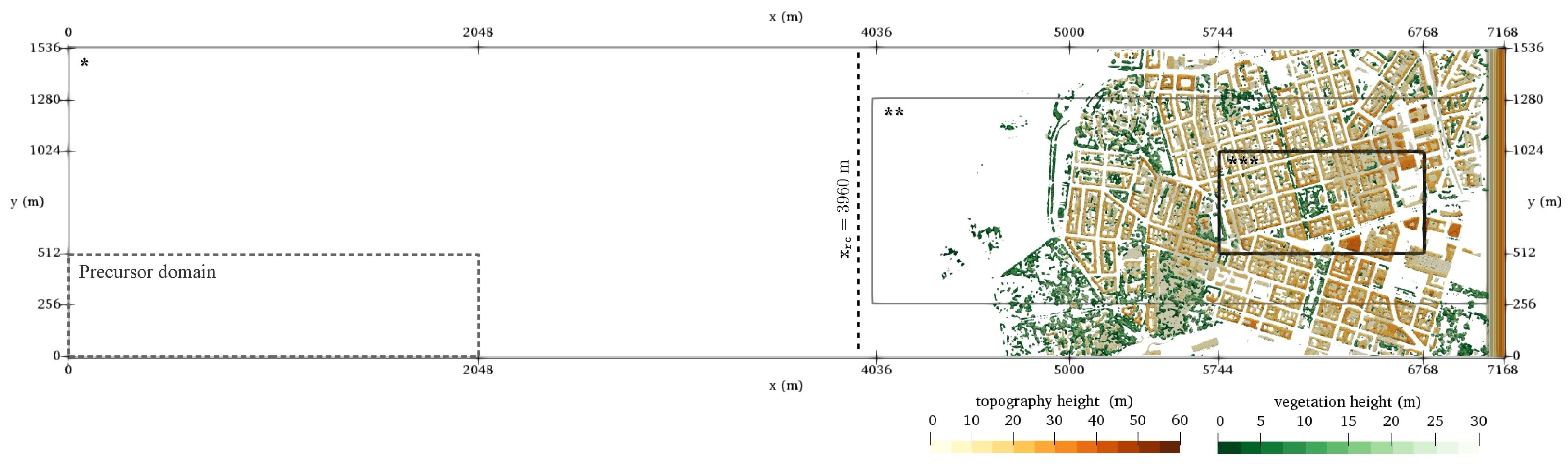
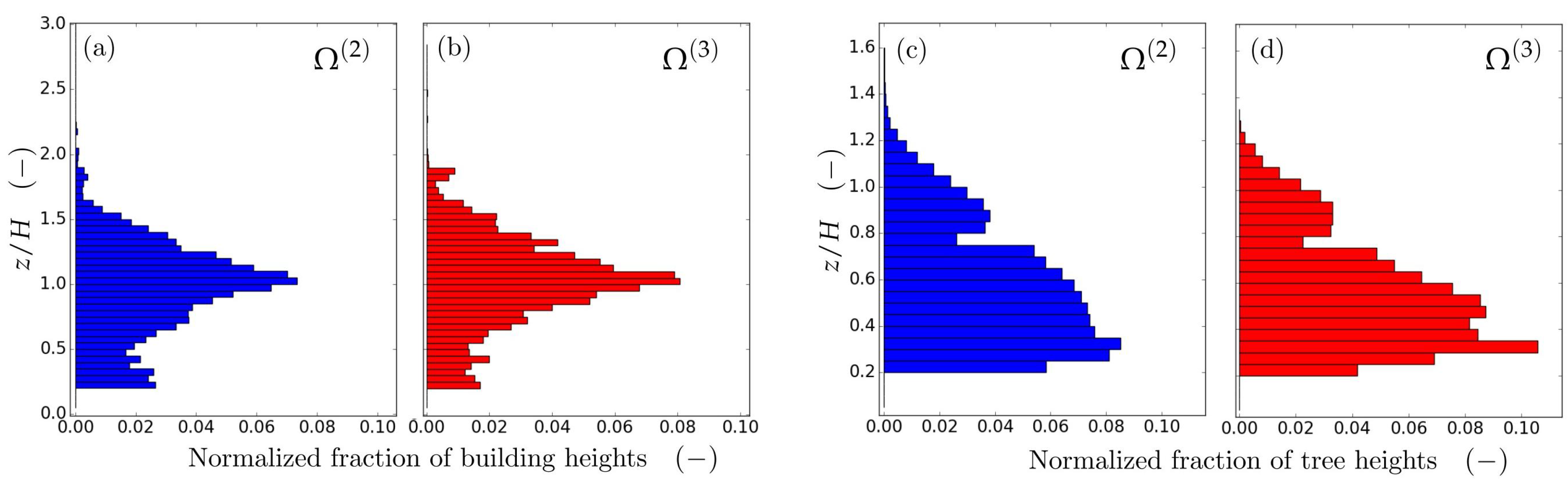
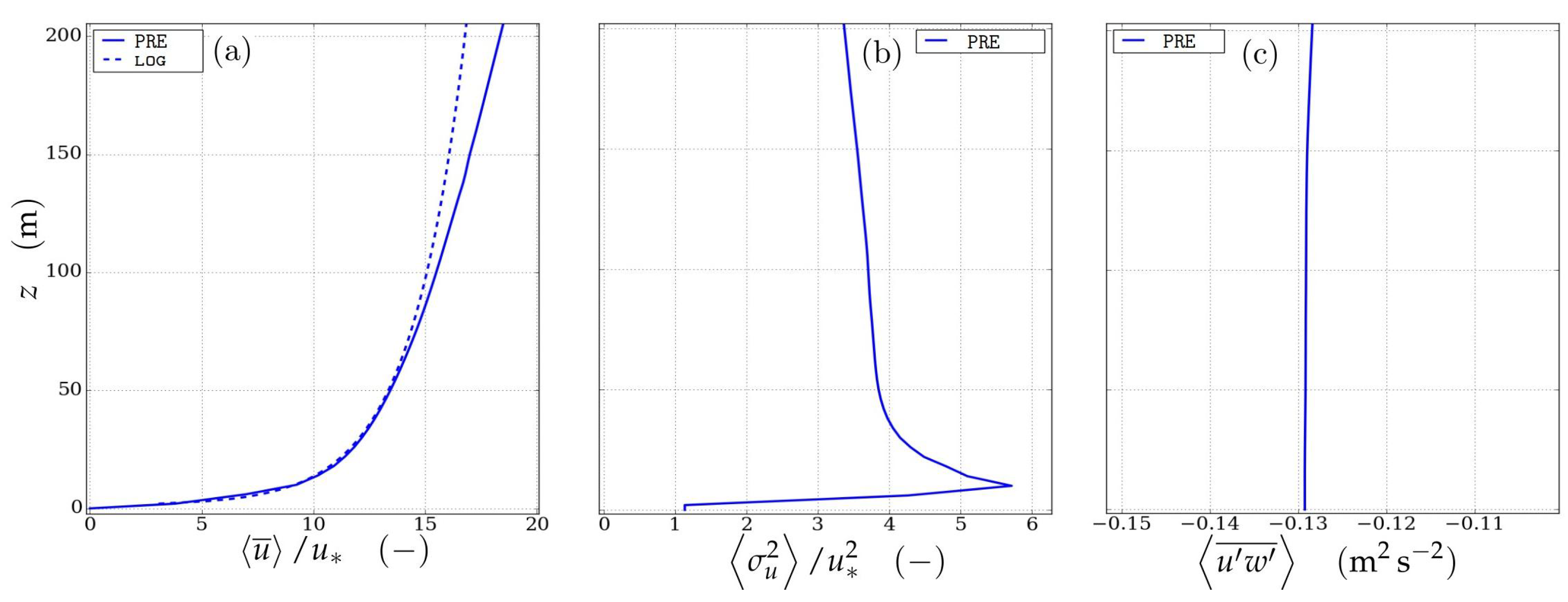
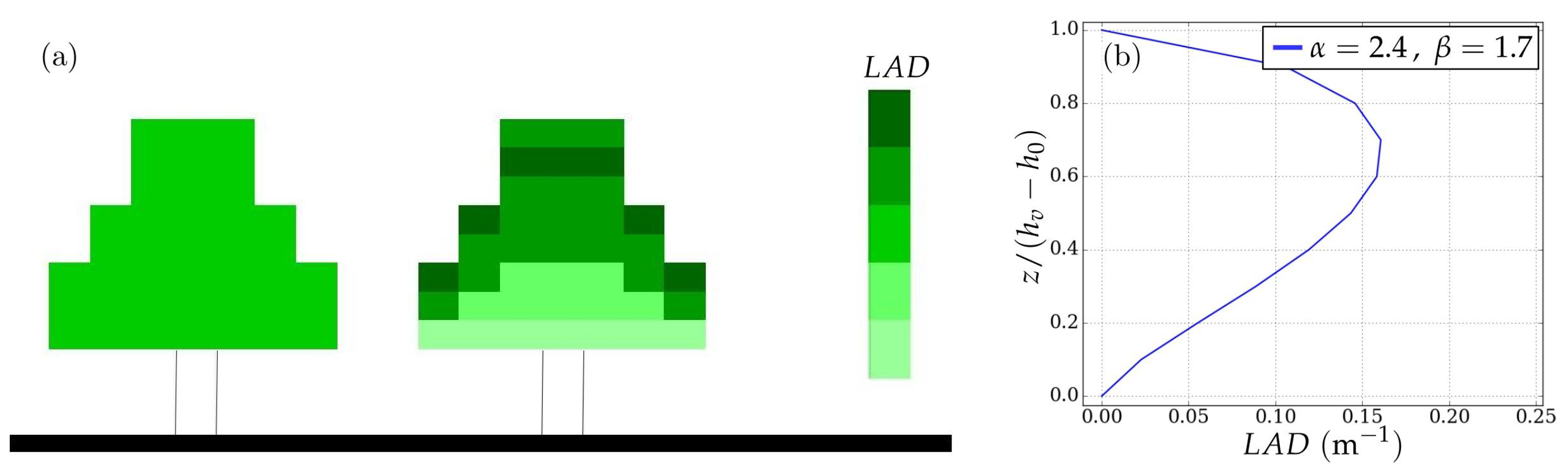
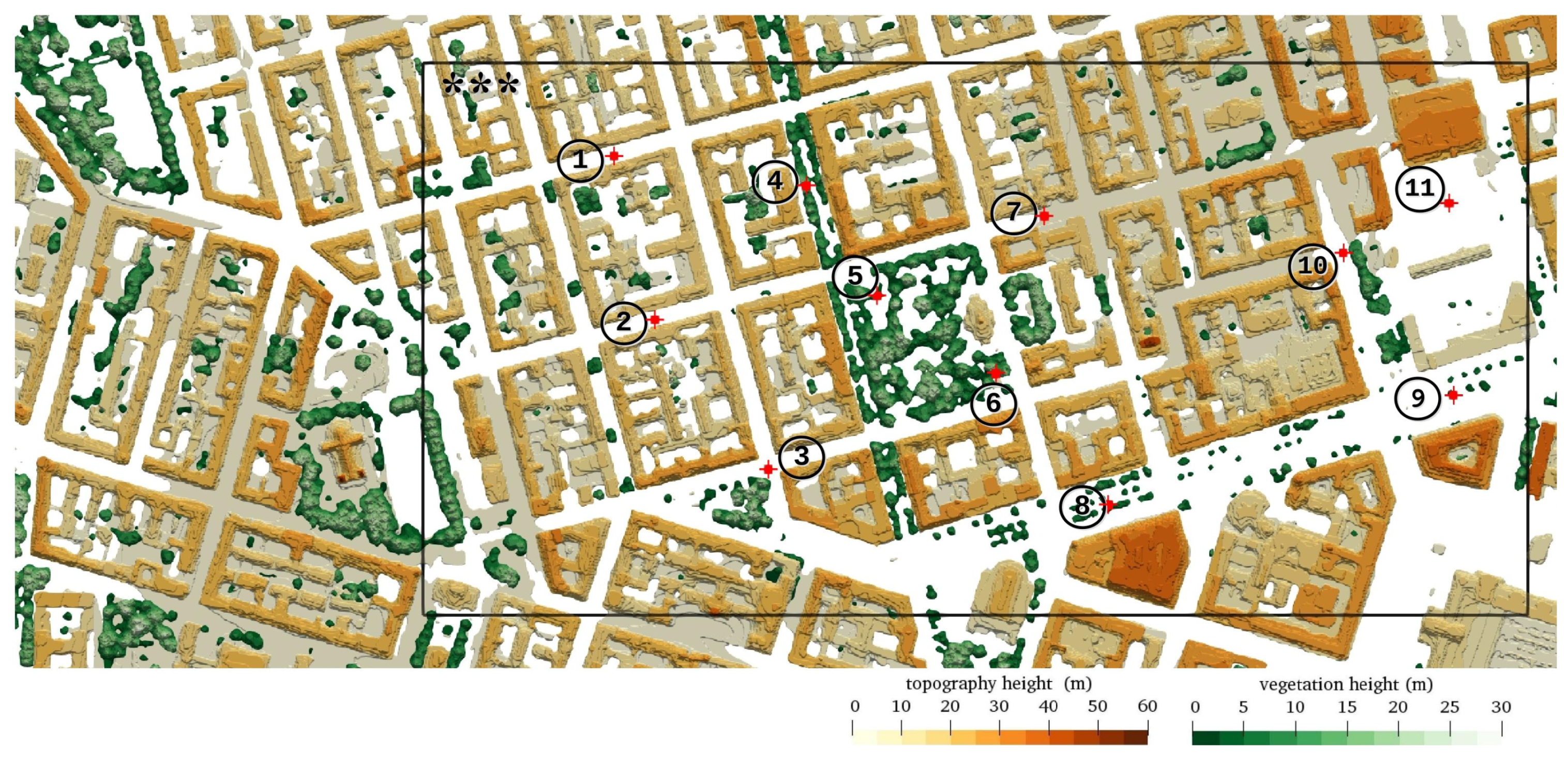
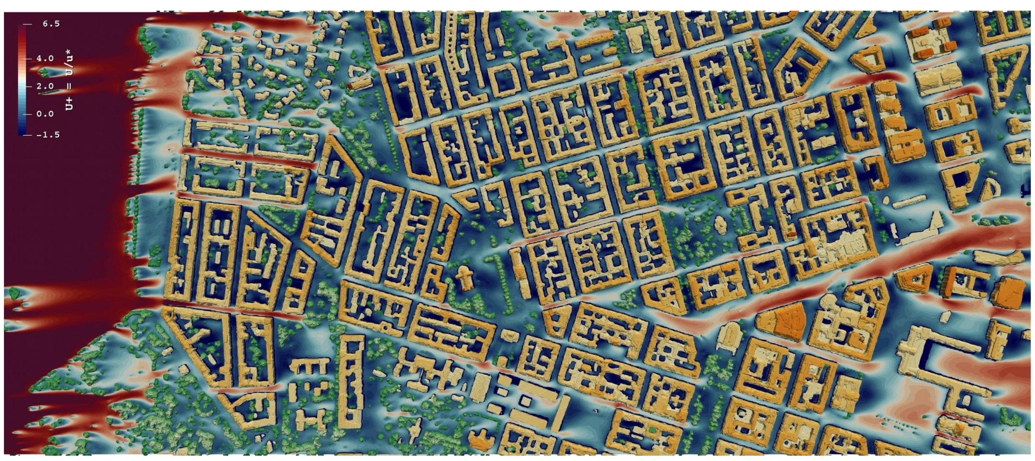
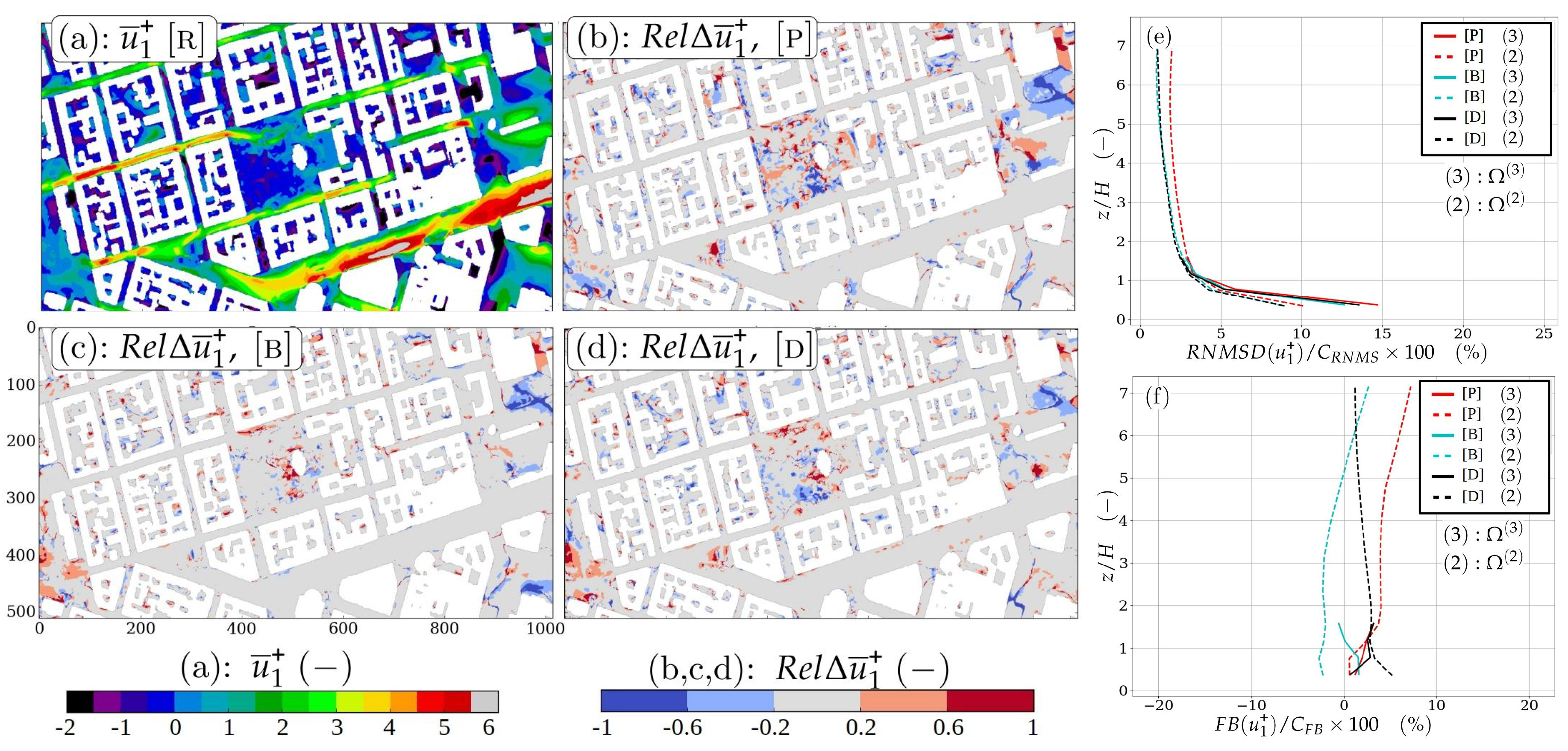
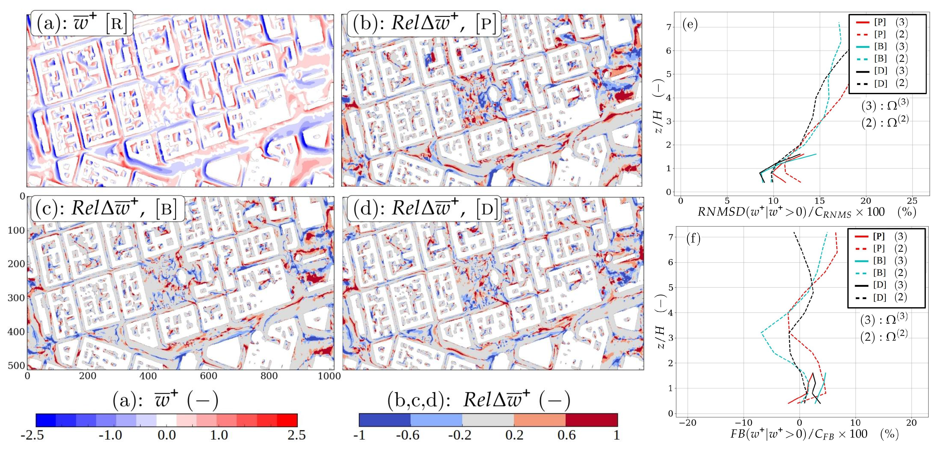
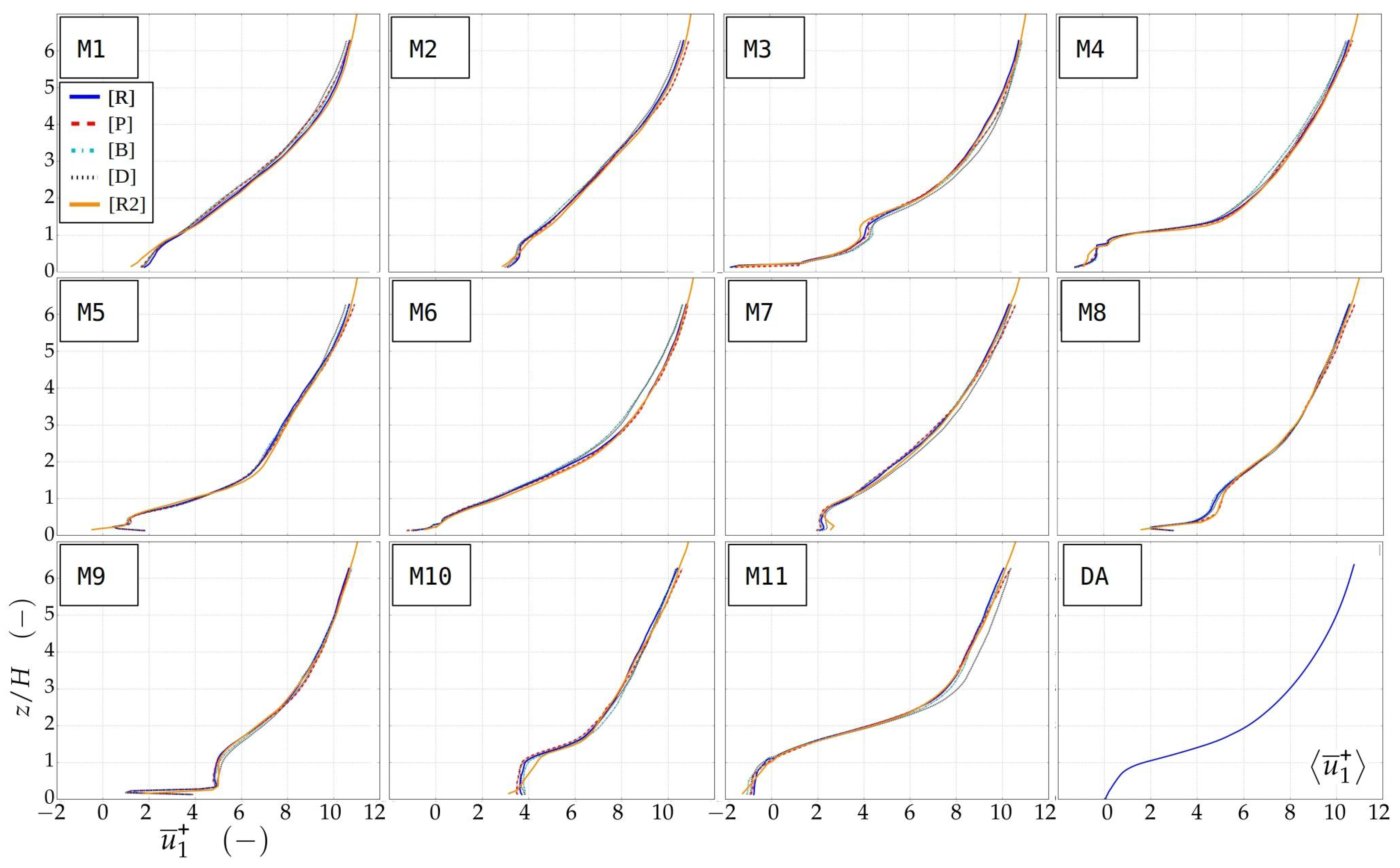
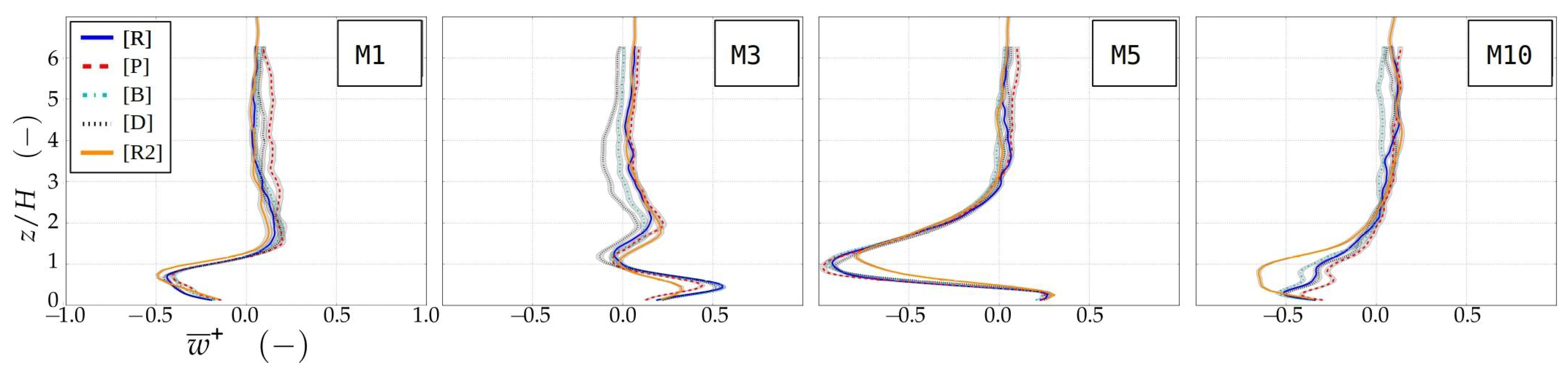
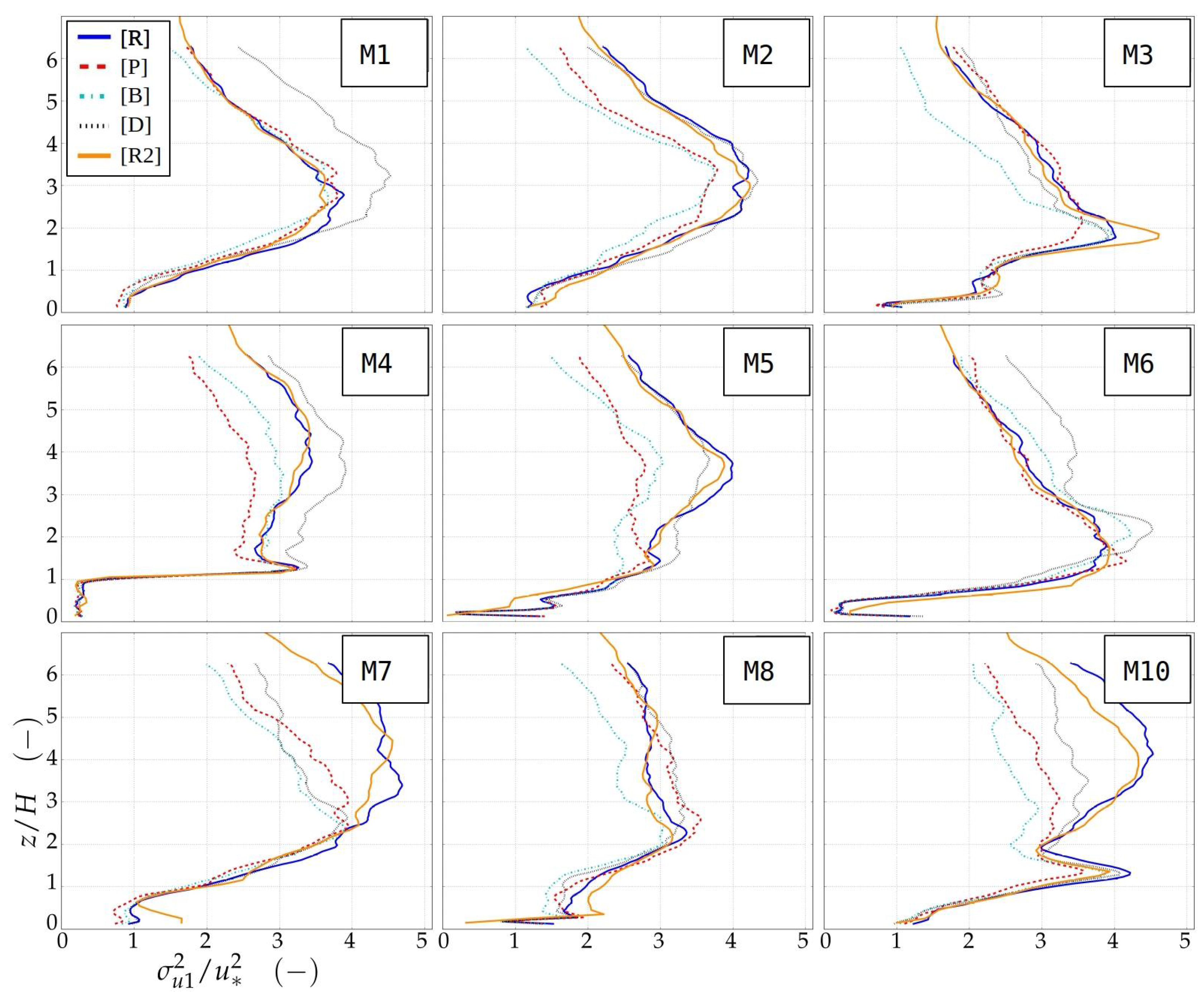
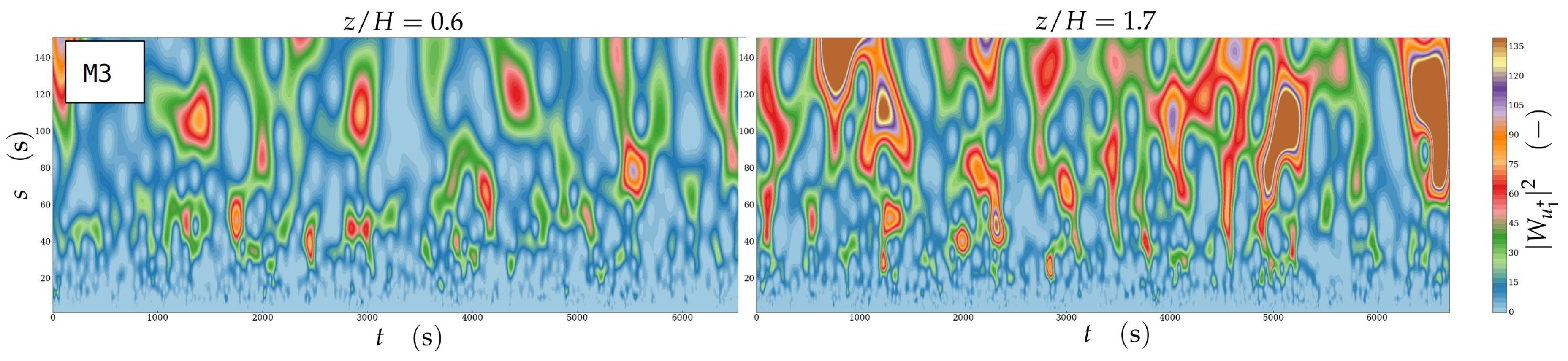
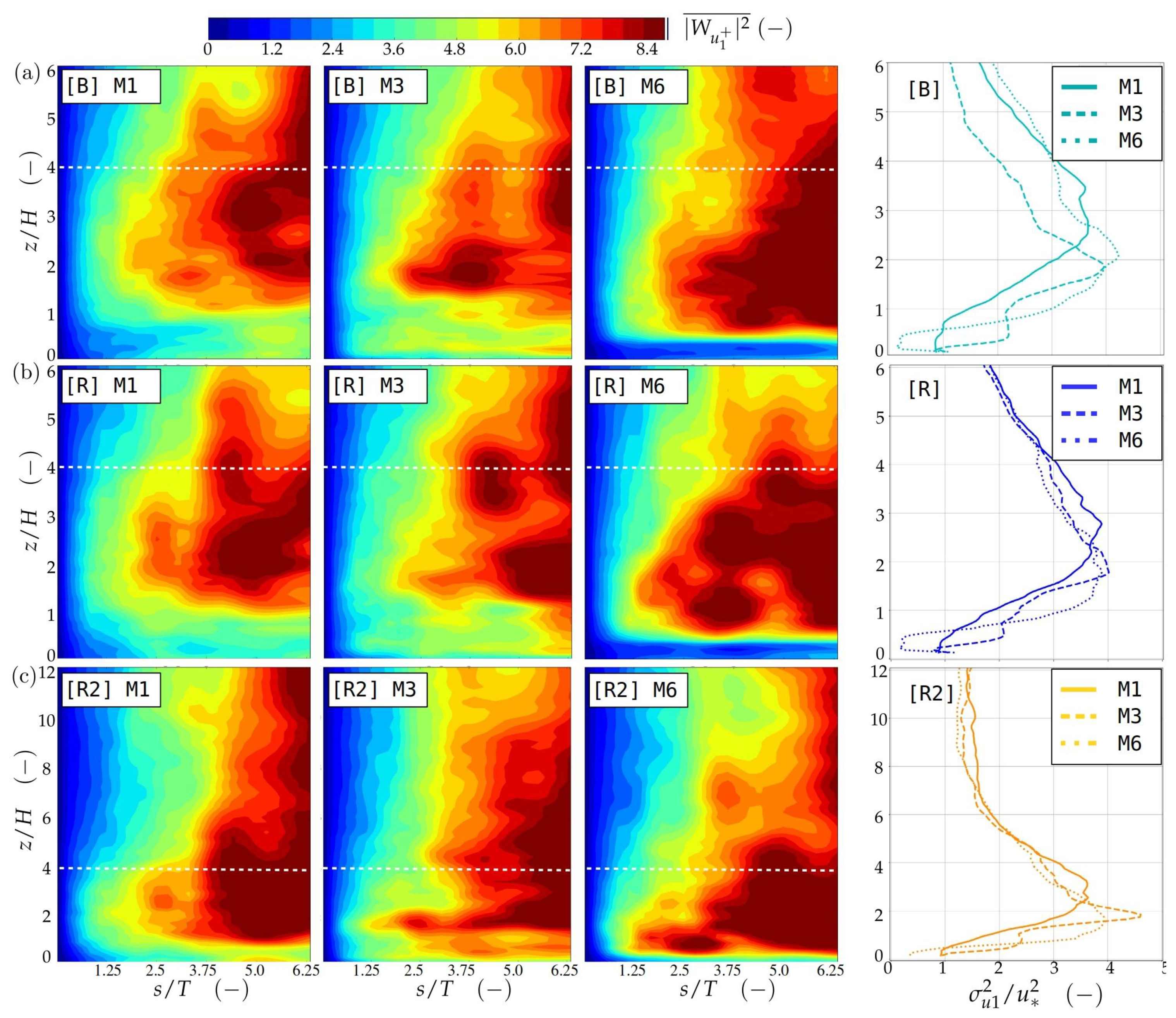
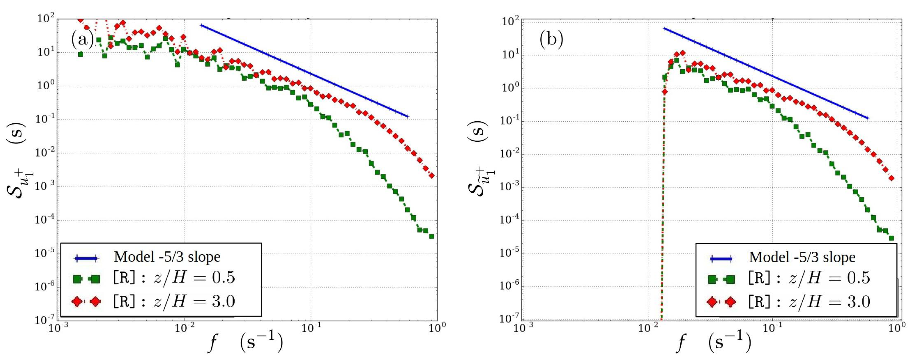
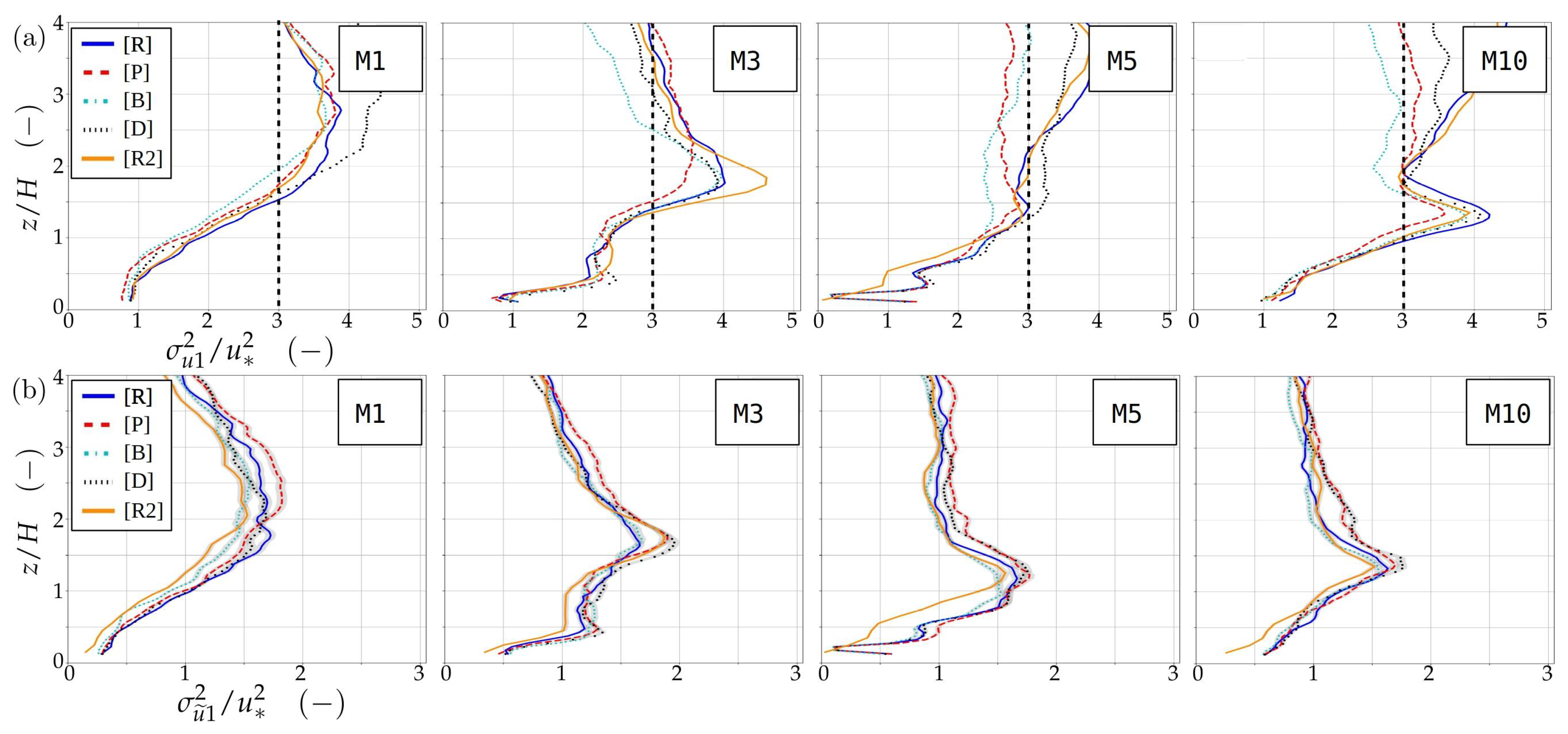
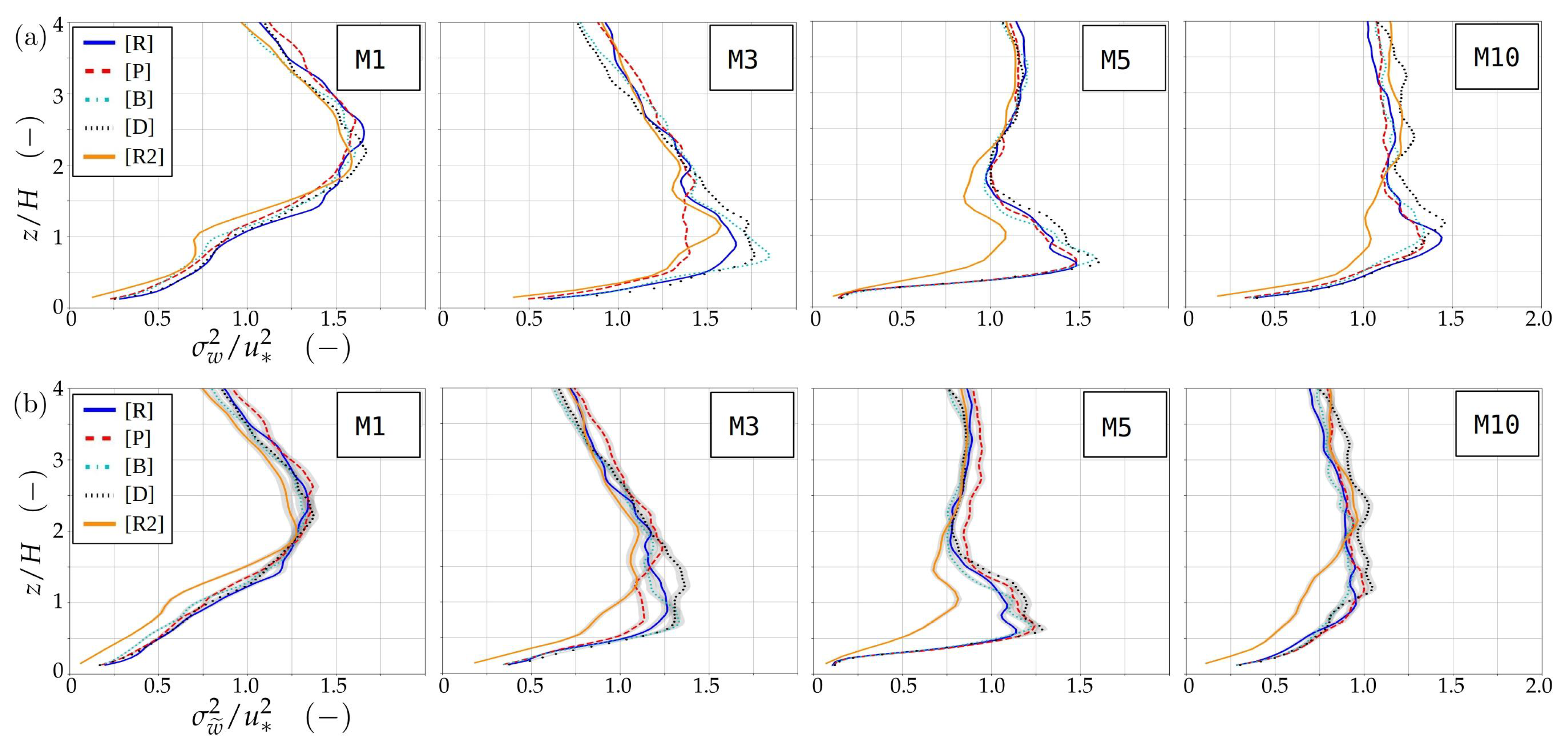
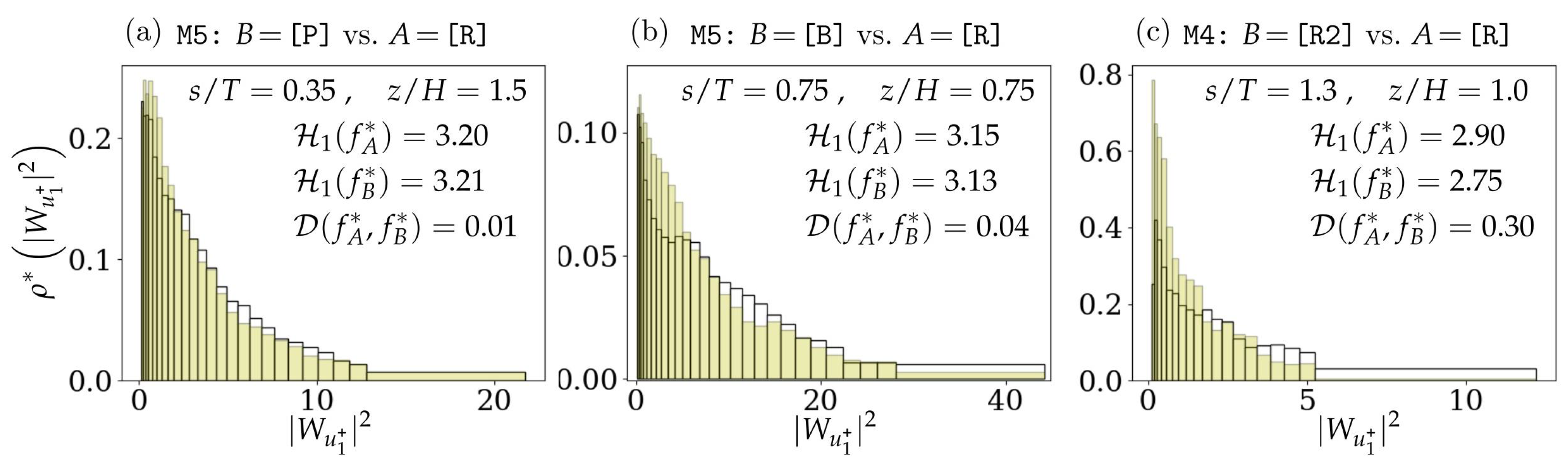
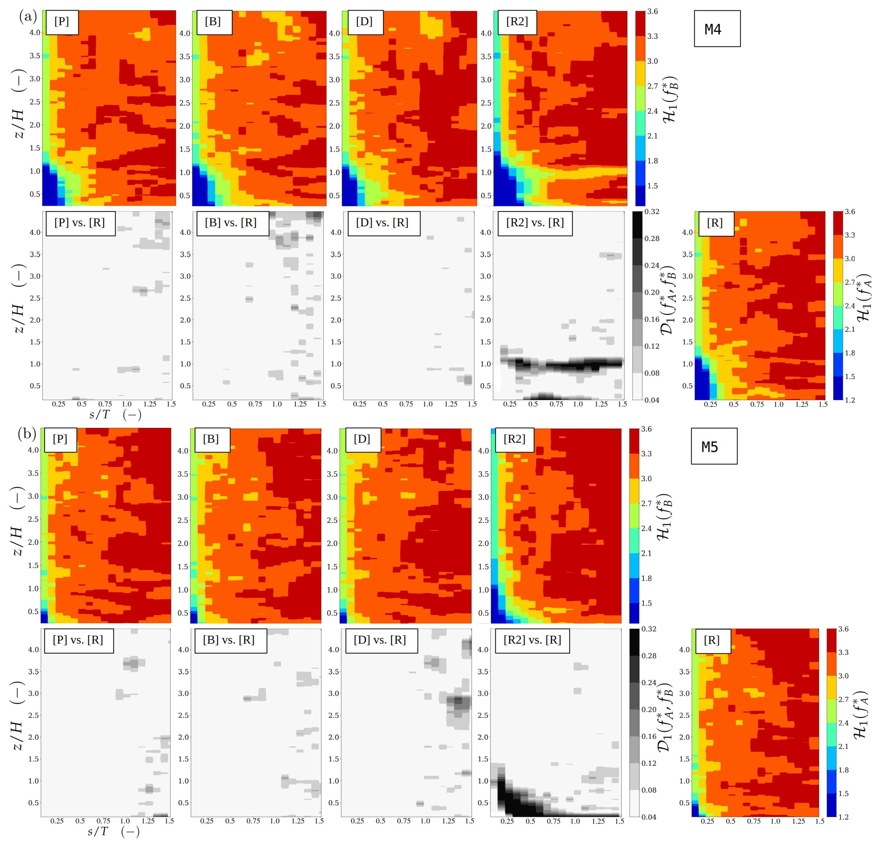
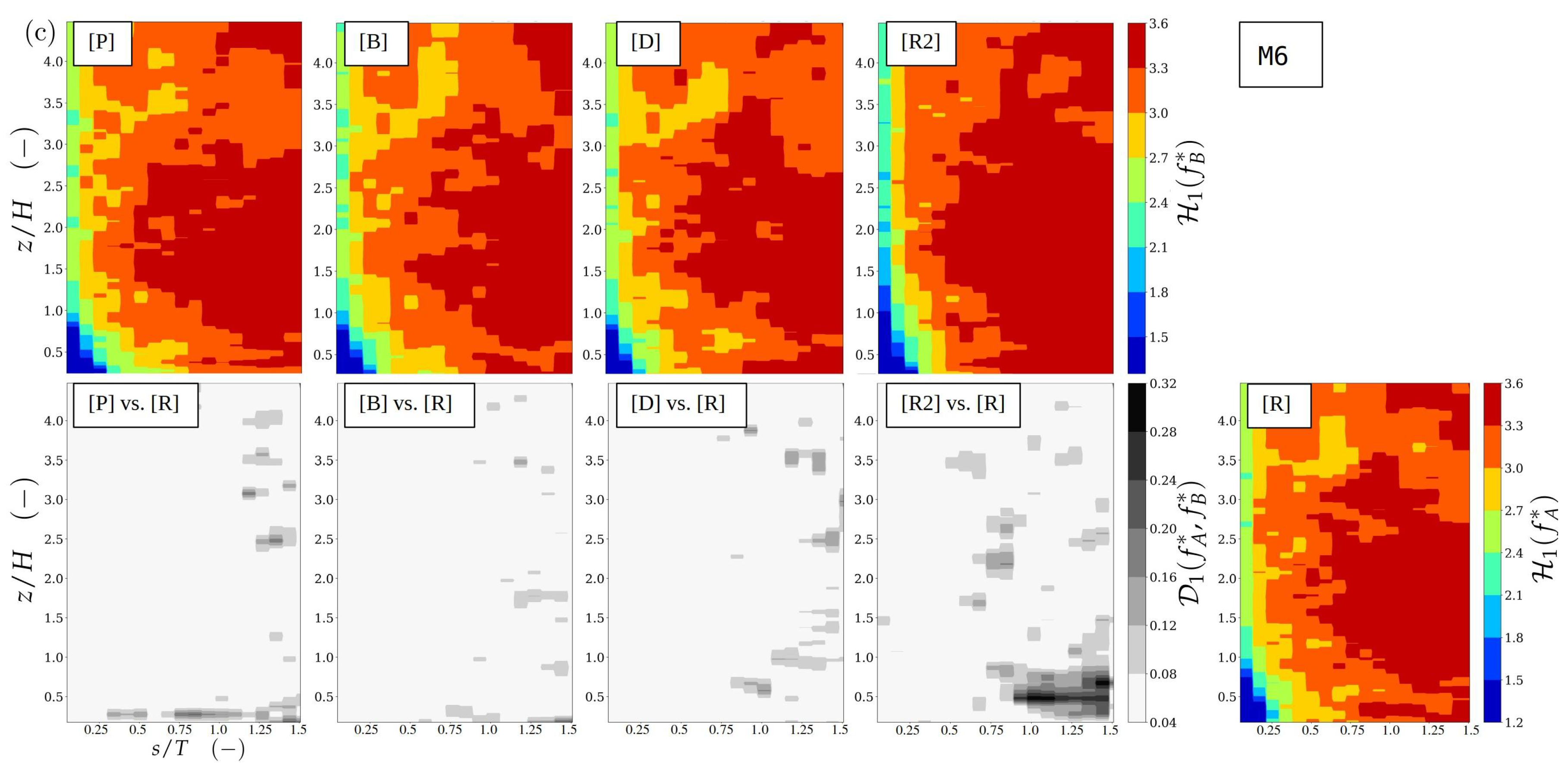
Table 1.
Dimensions and grid specifications for the nested Large-Eddy Simulation (LES) domains.
| Domain dimensions | 7168 m | 3072 m | 1024 m | |
| 1536 m | 1024 m | 512 m | ||
| 512 m | 256 m | 128 m | ||
| Cell size | 4 m | 2 m | 1 m | |
| Domain node counts | 1792 | 1536 | 1024 | |
| 384 | 512 | 512 | ||
| 128 | 128 | 128 | ||
| Total domain node count | ||||
| Nested model node count | ||||
Table 2.
Summary of morphometric statistics for the urban area: Separate values are listed for the area within but outside of and within alone.
Table 2.
Summary of morphometric statistics for the urban area: Separate values are listed for the area within but outside of and within alone.
| Mean | building heights | m | m |
| tree heights | m | m | |
| Characteristic canopy height | m | ||
| Std. of | building heights | m | m |
| tree heights | m | m | |
| Plan area fractions of | buildings | ||
| trees | |||
| Frontal area fractions of | buildings | ||
| trees | |||
Table 3.
A listing of all the LES cases included in this study and their respective modification presented in juxtaposition to the reference configuration.
Table 3.
A listing of all the LES cases included in this study and their respective modification presented in juxtaposition to the reference configuration.
| Model Constituent | Reference Case | Modified Case |
|---|---|---|
| LAD profile: | [R]: | [P]: |
| for and | ||
| Drag coefficient: | [R]: | [D]: |
| Neutral ABL height: | [R]: | [B]: |
Table 4.
Similarity scaling parameters from the different computational cases.
| Case | Friction Velocity | Roughness ength | Displacement Height |
|---|---|---|---|
| [R] | 0.539 | 0.063 | 1.08 |
| [P] | 0.521 | 0.063 | 1.08 |
| [B] | 0.505 | 0.067 | 1.05 |
| [D] | 0.535 | 0.066 | 1.04 |
© 2020 by the authors. Licensee MDPI, Basel, Switzerland. This article is an open access article distributed under the terms and conditions of the Creative Commons Attribution (CC BY) license (http://creativecommons.org/licenses/by/4.0/).
Share and Cite
MDPI and ACS Style
Auvinen, M.; Boi, S.; Hellsten, A.; Tanhuanpää, T.; Järvi, L. Study of Realistic Urban Boundary Layer Turbulence with High-Resolution Large-Eddy Simulation. Atmosphere 2020, 11, 201. https://0-doi-org.brum.beds.ac.uk/10.3390/atmos11020201
AMA Style
Auvinen M, Boi S, Hellsten A, Tanhuanpää T, Järvi L. Study of Realistic Urban Boundary Layer Turbulence with High-Resolution Large-Eddy Simulation. Atmosphere. 2020; 11(2):201. https://0-doi-org.brum.beds.ac.uk/10.3390/atmos11020201
Chicago/Turabian StyleAuvinen, Mikko, Simone Boi, Antti Hellsten, Topi Tanhuanpää, and Leena Järvi. 2020. "Study of Realistic Urban Boundary Layer Turbulence with High-Resolution Large-Eddy Simulation" Atmosphere 11, no. 2: 201. https://0-doi-org.brum.beds.ac.uk/10.3390/atmos11020201
Note that from the first issue of 2016, this journal uses article numbers instead of page numbers. See further details here.