A Synergistic Effect of Blockings on a Persistent Strong Cold Surge in East Asia in January 2018

Abstract

A persistent strong cold surge occurred in East Asia in late January 2018, causing mean near-surface air temperature in China to hit the second lowest since 1984. Moreover, the daily mean air temperature remained persistently negative for more than 20 days. Here, we find that a synergistic effect of double blockings in Western Europe and North America plays an important accelerating role in the rapid phase transition of Arctic Oscillation and an amplifying role in the strength of cold air preceding to the cold surge outbreaks by the use of an isentropic potential vorticity analysis. In mid-January, an Atlantic mid-latitude anticyclone merged with Western Europe blocking, which led to a strengthening of the blocking. Simultaneously, the Pacific-North American blocking was also significantly strengthened. The two blockings synchronously deeply stretched towards the Arctic, which resulted in, on the one hand, warm and moist air of the Pacific and the Atlantic being excessively transported into the Arctic, and on the other hand, the polar vortex being split and cold air being squeezed southwards and accumulating extensively on the West Siberian Plain. After the breakdown of the double blocking pattern, which lasted for about 10 days, the record-breaking cold surge broke out in East Asia. It was discovered that the synergistic effect of double blockings extending into the Arctic, which is conducive to extreme cold events, has been rapidly increasing in recent years.

1. Introduction

In the context of global warming, Arctic temperatures have increased rapidly and Arctic sea ice continues to melt [1,2,3]. In the meantime, the frequency of extreme cold in the mid-latitudes of the northern hemisphere is increasing, especially in Eurasia [4,5,6]. The main reasons for cold extremes in Eurasia are reported as Arctic circulation changes (such as Arctic Oscillation (AO)) [7,8], sea ice melting [9,10,11,12], Arctic warming [6,13,14,15], tropical driving [16], and Eurasian snow cover anomalies [7,17,18]. Regardless of the mechanism used, Arctic systems and their interactions with atmospheric systems in different latitudes are key to understanding the reasons for extreme events in winter Eurasia. The blocking is the channel for direct communication between the mid-latitudes and the Arctic [19,20]. When the Ural blocking shows a quasi-steady characteristic, cold air is continuously conveyed to the mid-latitude continent under the guidance of the blocking, which is conducive to cold extremes in Eurasia [21,22,23]. Furthermore, the dipole circulation of the northern low potential vorticity (PV) (blocking) and the southern high PV (polar vortex) in the Eurasian region [24], and the co-evolution of the Ural blocking and the western North America blocking are crucial for the formation of a cold extreme [25].

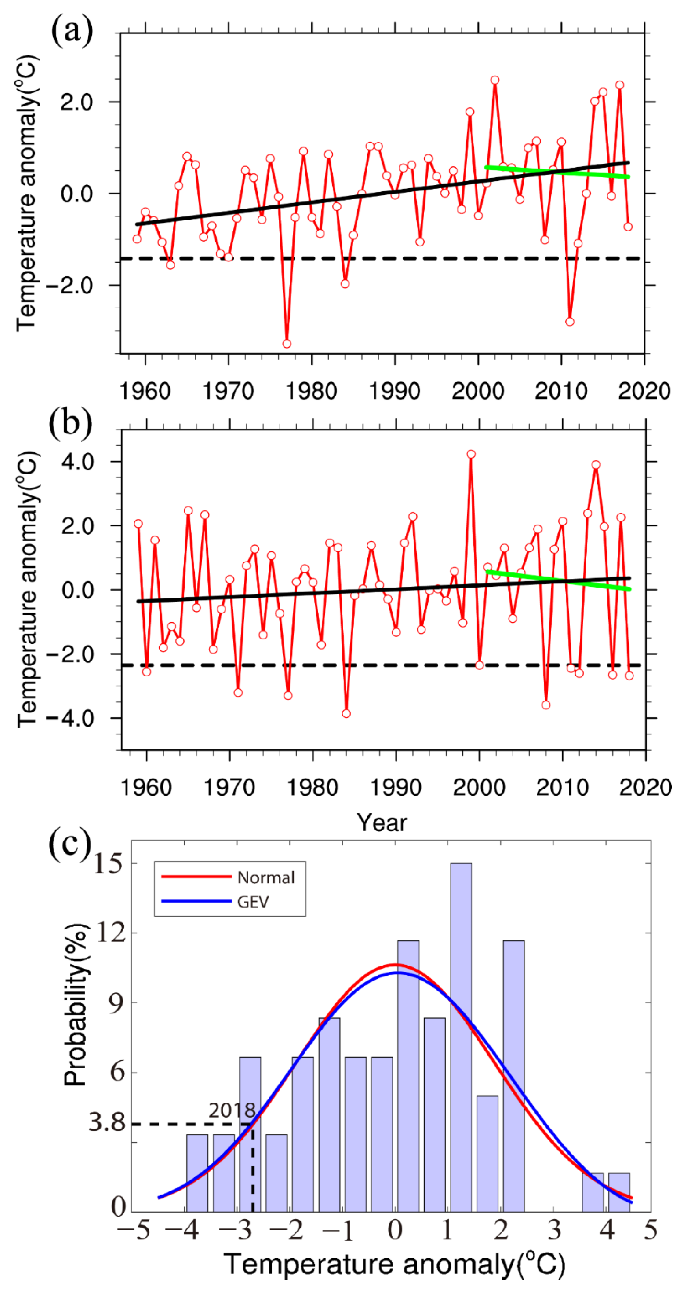
While East Asia’s mean temperature has continuously risen from 1959 to 2018, it has seen a downward trend in recent years. As shown in Figure 1a, January temperature time series of China have a long-term warming trend despite the cooling trend in the last 18 years. The coldest January occurred in 1977. Although the air temperature in January of 2018 is not very low, we find that late January 2018 experienced extremely low air temperature (Figure 1b) due to a strong cold surge. Figure 1b also shows that although the near-surface temperature in China in late January has generally increased in the past 60 years, it has shown a notable trend difference in the last 18 years since 2001. Furthermore, temperature changes are getting more and more intense and extremely low temperature values occur more frequently than before. In the last 18 years, since 2001, the temperature anomaly has been below −2.35 °C (−1.25 standard deviation) five times, although it has also only been this low five times in the 42 years before 2001 (1959–2000).

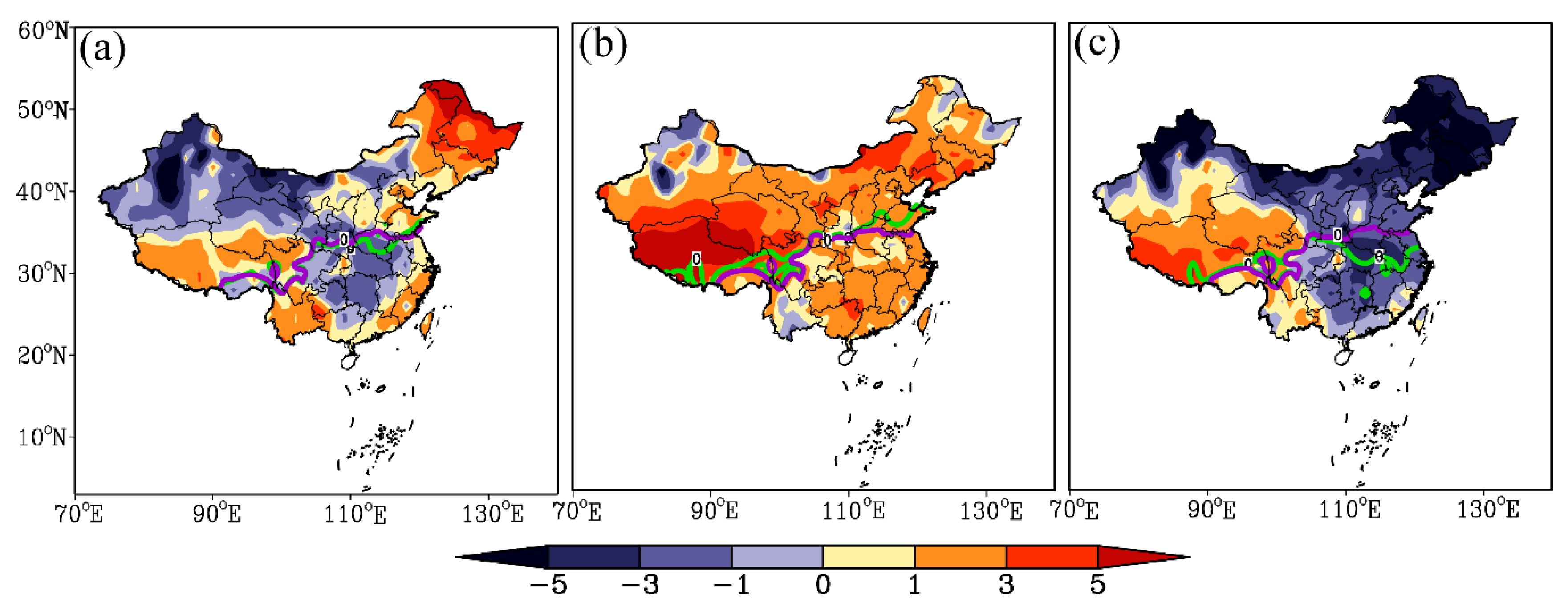
In early and late January 2018, there were two cold surges in China and the second was stronger than the first (Figure 2). The strong cold surge caused persistent low temperature, rain, and snowy weather. Except the western plateau region, there was a substantial temperature decline in China in late January (Figure 2c). The near-surface air temperature contour of 0 °C in late January 2018 deviated from the climatological position and moved obviously southward. The China surface temperature anomaly in late January 2018 was the second lowest in the same period in the past 34 years (since 1985), second only to 2008 (Figure 1b). Furthermore, probability density function of the late January surface temperature anomalies from 1959 to 2018 in China shows that the actual probability in a bar chart is 6.7% and the probability of fitting in late January 2018 is 3.8% (Figure 1c). This suggests that the intensity of this cold surge reached a rare level in history, but there has been no systematic study on this cold surge. Therefore, in this paper, we used an isentropic PV, a powerful tool for analyzing winter weather events [26], to study the reasons and early signals of this cold surge.

2. Data and Method

2.1. Data

The surface temperature data from 1959 to 2018 were taken from the National Meteorological Information Center of the China Meteorological Administration based on recorded observations from 699 meteorological stations. The potential temperature at tropopause ($\mathrm{P}\mathrm{V}=2\mathrm{P}\mathrm{V}\mathrm{U}$, $1\mathrm{P}\mathrm{V}\mathrm{U}={10}^{-6}·{\mathrm{m}}^2·\mathrm{K}·{\mathrm{s}}^{-1}·{\mathrm{kg}}^{-1}$, the same below) was taken from the ERA-Interim reanalysis project [26] at the European Centre for Medium-Range Weather Forecasts (ECMWF). Fields of temperature, geopotential height and meridional/zonal wind were obtained from the National Center for Environmental Protection (NCEP)/National Center for Atmospheric Research (NCAR) Reanalysis Project [27].

2.2. Method

2.2.1. Isentropic Potential Vorticity

The vertical component of isentropic PV is calculated by the following Equation [28]:

$$P{V}_p=-g({\zeta }_{\theta }+f)\frac{\partial \theta }{\partial p}$$

(1)

$P{V}_p$, hereinafter is referred to as isentropic PV. Where $g$ is the gravity acceleration, ${\zeta }_{\theta }$ is the vertical component of the relative vorticity on the isentropic surface, f is the Coriolis parameter (planetary vorticity), and $-\frac{\partial \theta }{\partial p}$ is the static stability.

Firstly, we calculate the potential temperature, vorticity and static stability on each isostatic surface and then linearly interpolate the fields onto each isentropic surface with a 5 K interval from 275 K to 375 K. Finally, we calculate the isentropic PV according to Equation (1).

2.2.2. The Dynamic Blocking Index

The potential temperature of the tropopause is characterized by a cold polar region and a warm subtropical region. However, there is a meridional potential temperature gradient inversion when a blocking occurs. Thus, the dynamic blocking index ($\mathrm{P}\mathrm{V}-\theta$) at longitude $\lambda$ is defined as the difference in the average potential temperature between the north and south regions of blocking at tropopause ($\mathrm{P}\mathrm{V}=2\mathrm{P}\mathrm{V}\mathrm{U}$) [29]:

$$B=\frac{2}{\Delta \varphi }{\displaystyle {\int }_{{\varphi }_0}^{{\varphi }_0+\Delta \varphi /2}\theta }d\varphi -\frac{2}{\Delta \varphi }{\displaystyle {\int }_{{\varphi }_0-\Delta \varphi /2}^{{\varphi }_0}\theta }d\varphi$$

(2)

where $\theta$ is the potential temperature, ${\varphi }_0={\varphi }_c(\lambda )\pm \epsilon$, ${\varphi }_c(\lambda )$ is the annual mean central blocking latitude, $\epsilon {=4}^{°}$ and $\Delta \varphi$ is a typical meridional scale for blocking ($\Delta \varphi {=30}^{°}$) (Obtained [29]). We calculate three blocking indices on the three latitudes (${\varphi }_0={\varphi }_c(\lambda )$, ${\varphi }_0={\varphi }_c(\lambda )+\epsilon$ and ${\varphi }_0={\varphi }_c(\lambda )-\epsilon$) at the longitude $\lambda$ and then select the maximum of the three indices as the actual blocking index. When $B>0$, the longitude $\lambda$ could be said to be blocked, indicating that there is a high $\theta$ in the north and a low $\theta$ in the south.

2.2.3. The Diabatic Heating

Diabatic heating is calculated by an inverse algorithm according to the thermodynamic equation [30,31]:

$$\frac{\partial T}{\partial t}=-v\cdot \nabla {\rm T}+\omega \sigma +\frac{Q_1}{C_p}$$

(3)

where $t$ is time, $T$ is temperature, $v$ represents the horizontal velocity vector, $\nabla$ denotes the horizontal gradient operator, $\sigma =\left(\frac{RT}{C_{p}P}\right)-\left(\frac{\partial T}{\partial P}\right)$ is the static stability, and $\omega$ is the vertical velocity. $R$ is the gas constant, $P$ is pressure, $Q_1$ indicates the atmospheric apparent heat source, and $C_p$ is the specific heat at constant pressure.

3. Results

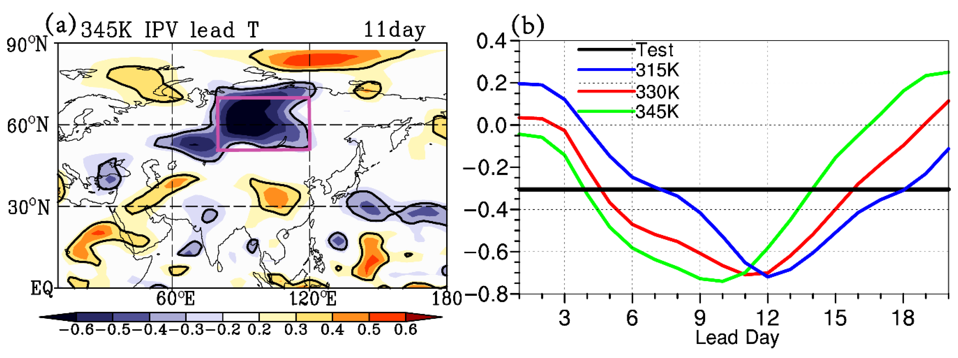
The strong cold surge occurred in East Asia in late January 2018, causing strong and persistent low temperature, rain, and snowy weather; the lowest temperature averaged over China occurred on January 28. Tracking the PV source that affected the cold surge in January 2018, we found that the West Siberian Plain (80–120° E, 50–70° N) was the direct source of high PV. The lowest value of the leading correlation coefficient is about −0.7 when the daily isentropic PV series averaged over the region was about 11 days ahead of the daily mean China near-surface temperature series. At that time, the main significant leading correlation regions is the West Siberian Plain (see Figure 3) and the significant negative correlations lasted for about 10 days (from leading about 15 days to leading about 5 days), implying that cold air likely accumulated here. The West Siberian Plain was also found to be a key region where extratropical waves are deflected from the extratropical regions and travel toward the western Pacific, as reported by Liess et al. [32].

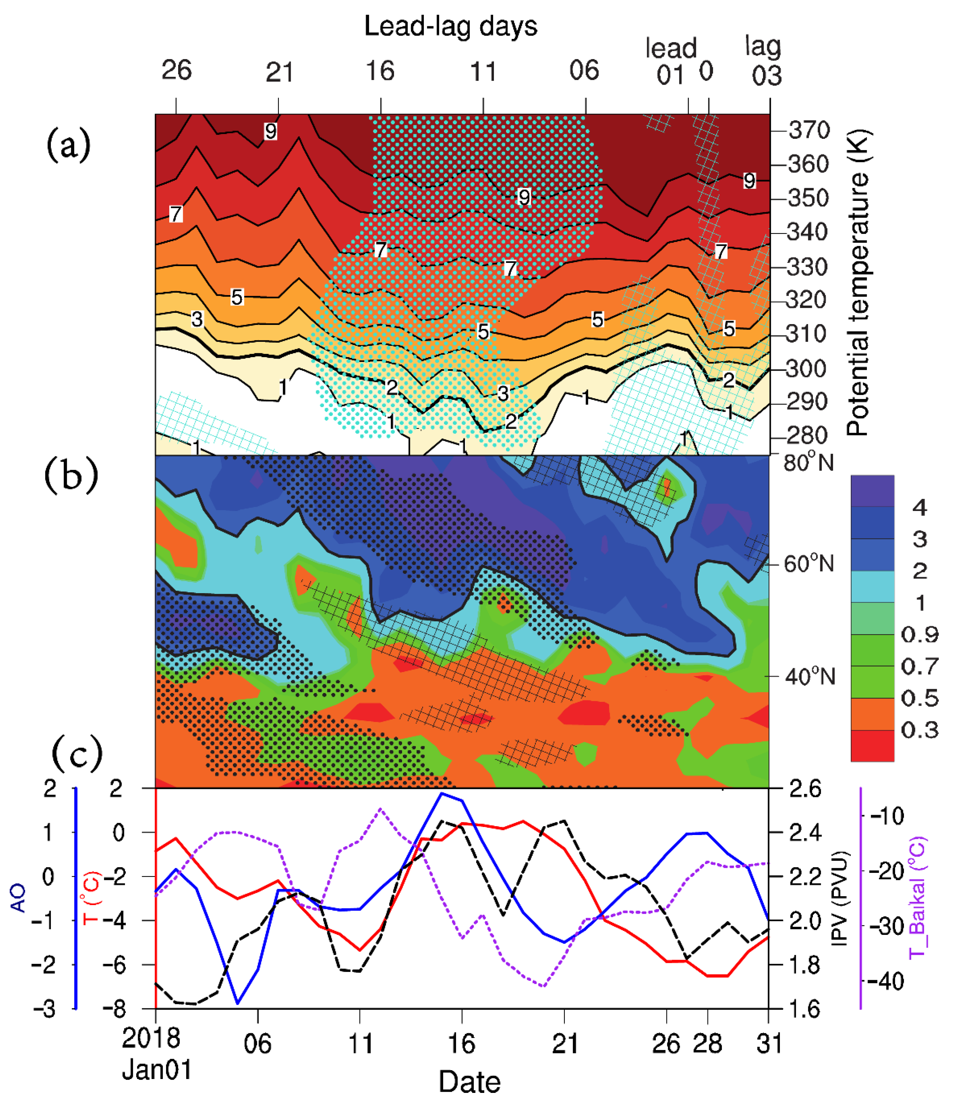
As shown in Figure 4, high PV over the direct source region stretched vertically downward and moved southward since about 10 January, the PV had the lowest temperature for about 18 days. The 2 PV contour representing dynamic tropopause fell from 305 K to 275 K of isentropic surface, whose change feature is very coincident with the local 1000 hPa temperature curve (the purple dotted line in Figure 4c). On January 20, when the high PV stretched to the lowest level, the temperature at 1000 hPa also dropped to the lowest value of −41 °C, indicating that the high PV corresponds to cold air. The latitude–time evolution map of cold air source (90° E) on the 305 K isentropic surface (Figure 4b) shows that the high PV moved from the Arctic to the direct source region of the West Siberian Plain, since the leading time was about 16 days. This phenomenon of cold air southward can be explained by the perspective of global meridional mass circulation [33,34,35,36]. Additionally, the 2 PVU contour hesitated at 50° N throughout the middle of January and reached 42° N on 28 January. Compared with the average 305 K isentropic PV curve (Figure 4c) in the West Siberian Plain (80–120° E, 50–70° N), we found that the PV over the direct source region increased in an oscillating manner following a downward propagation of high-level PV. The high PV increased rapidly here since 12 January and was maintained for about 10 days. In the meantime, the temperature in this area kept dropping for nearly 10 days, with a drop of more than 30 °C. This shows that the high PV has a long-term accumulation here, later forming a high PV reservoir, and this accumulation phenomenon is significantly correlated with the later East Asian strong cold surge. Such a strong and long-lasting extended-range PV anomaly signal is important for the occurrence of the later persistent strong cold surge. In addition, compared with the evolution of the AO index in the winter (the blue curve in Figure 4c), there was a reverse from positive to negative in the AO phase before both the two cold surges occurred in January 2018 (the AO index leads China surface temperature by 3–7 days). The AO index changed sharply from the lowest value on 5 January (−2.89) to the highest value in the winter (1.88 on 15 January). The change range was above 4.7. The AO quickly declined and became negative on 18 January and then reached the lowest value on 21 January. Since then, the temperature over China began to decrease and reached the bottom of the valley on the 28th. Obviously, exploring why AO phase dramatically changed and high PV continuously accumulated will be valuable for the extended-range prediction of strong cold surges.

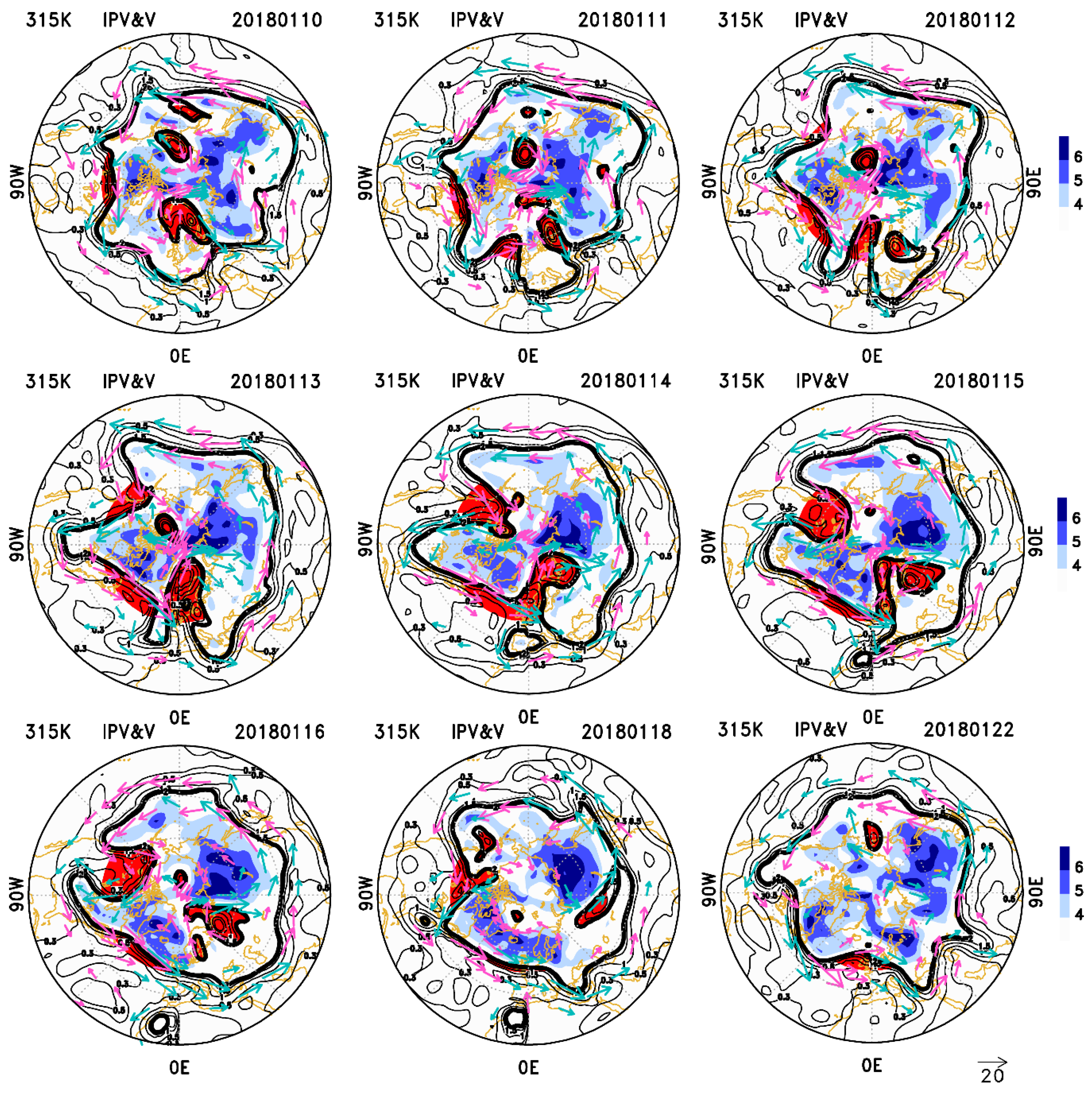
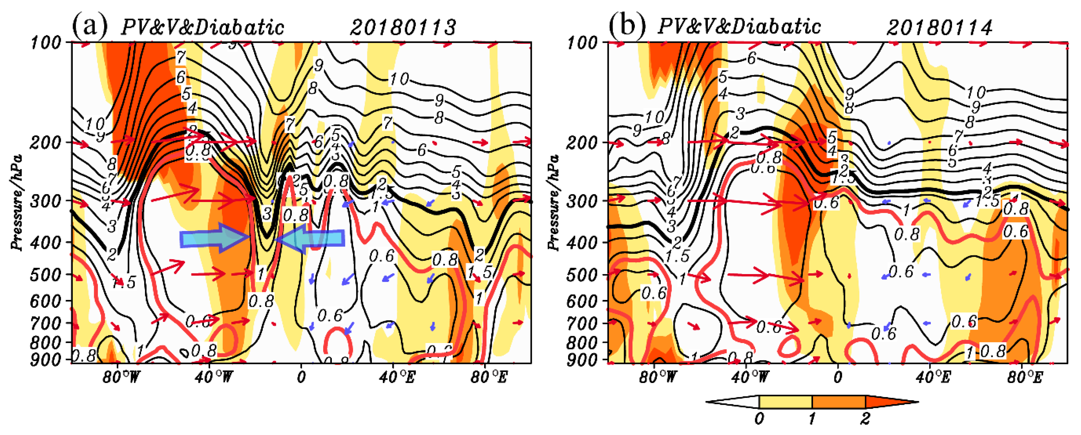
Isentropic PV can clearly characterize and track the evolution of systems such as mid-high latitude polar vortex and blocking [28,37,38,39,40,41]. We thus used the isentropic PV field to further analyze the driving factors and mechanisms of the high PV anomaly and the AO phase transition before the cold surge in late January 2018 (Figure 5). On 10 January, the 2 PVU contours were relatively flat. However, it should be noted that there was a strong high isentropic PV tongue in western North America extending to the mid-latitudes, which suggests a strong cold air process invading North America. Moreover, the high isentropic PV tongue stimulated the development of the downstream anticyclone. On the 11th, the isentropic PV contours in North America and the Atlantic became bent. On the 12th, both the blocking in Western Europe and the anticyclone in eastern North America strengthened and began to squeeze each other, resulting in large fluctuations in the 2 PVU contour. Warm air was transported to the Arctic upstream of the blocking ridges and cold air was transported to the mid-latitudes downstream of the blocking ridges. On the following day, the 13th, the Atlantic anticyclone in eastern North America continued to develop eastward, squeezed with the slow-moving Western European blocking, gradually cutting off North Atlantic high isentropic PV that stretched southward. On the 14th, the two anticyclones merged and formed a new strong blocking which stretched deeply from the mid-latitudes of the Atlantic to the Arctic, which formed a mid-high latitude transport channel of warm air. The Atlantic anticyclone still existed, connected to the blocking of Western Europe, and transported the warm and moist air of the Atlantic from the anticyclone’s rear to the blocking and then to the Arctic. This can be seen more clearly in Figure 6. On the 13th, two diabatic heating centers start to merge (light blue arrow) when two low PVs approached each other. On the 14th, they combined into one. Recent studies found that stronger warm air mass transported into the Arctic region is related with a stronger equatorward discharge of cold air in the lower troposphere, which is largely different from the result regarding weaker warm air mass transport [33,34,35,36]. Therefore, the strong warm air transport channel is very important to a strong cold surge. At this time, the Atlantic was in the positive phase of NAO and the strengthening of the Atlantic zonal westerly jet was beneficial to the dispersion downstream of Rossby wave, and the advection of the flow to the high-frequency PV may cause the weather scale wave to break [42], leading to the development and strengthening of the European blocking. Simultaneously, it is important to note that the blocking in western North America was also strongly developed to reach the Arctic, forming another transport channel of warm air; and it combined the European blocking together to squeeze the polar high PV and split the polar vortex into two centers, showing the shape of an “8”, one in northern Eurasia, and the other in near Greenland and North America. Although the high PV air at this time was split into two parts, it had not begun to go southward. On the 16th, as the Atlantic-Western European blocking moved eastward, the low PV was cut off and stayed in the high-latitude stratosphere in the Ural region, forming a closed anticyclone. This led the downstream high PV cold air to start a large-scale southward movement and in correspondence with this, the AO index began to sharply decline. On the 18th, the low PV anticyclone of Ural moved to the south side of high PV and showed a quasi-zonal pattern, forming a zonal trough with the north high PV, which caused a lot of cold air to accumulate behind the trough.

From the above analysis, on the extended-range scale, the Atlantic anticyclone caused by the North American cold surge interconnected with the European low PV blocking in mid-January, which formed the poleward transport channel of mid-latitude Atlantic warm and moist air. Importantly, the Western Europe blocking and North American blocking synergistically developed to the Arctic before the cold surge outbroke, which plays an important role in polar vortex splitting, AO phase transition, cold air accumulation, and a southward movement.

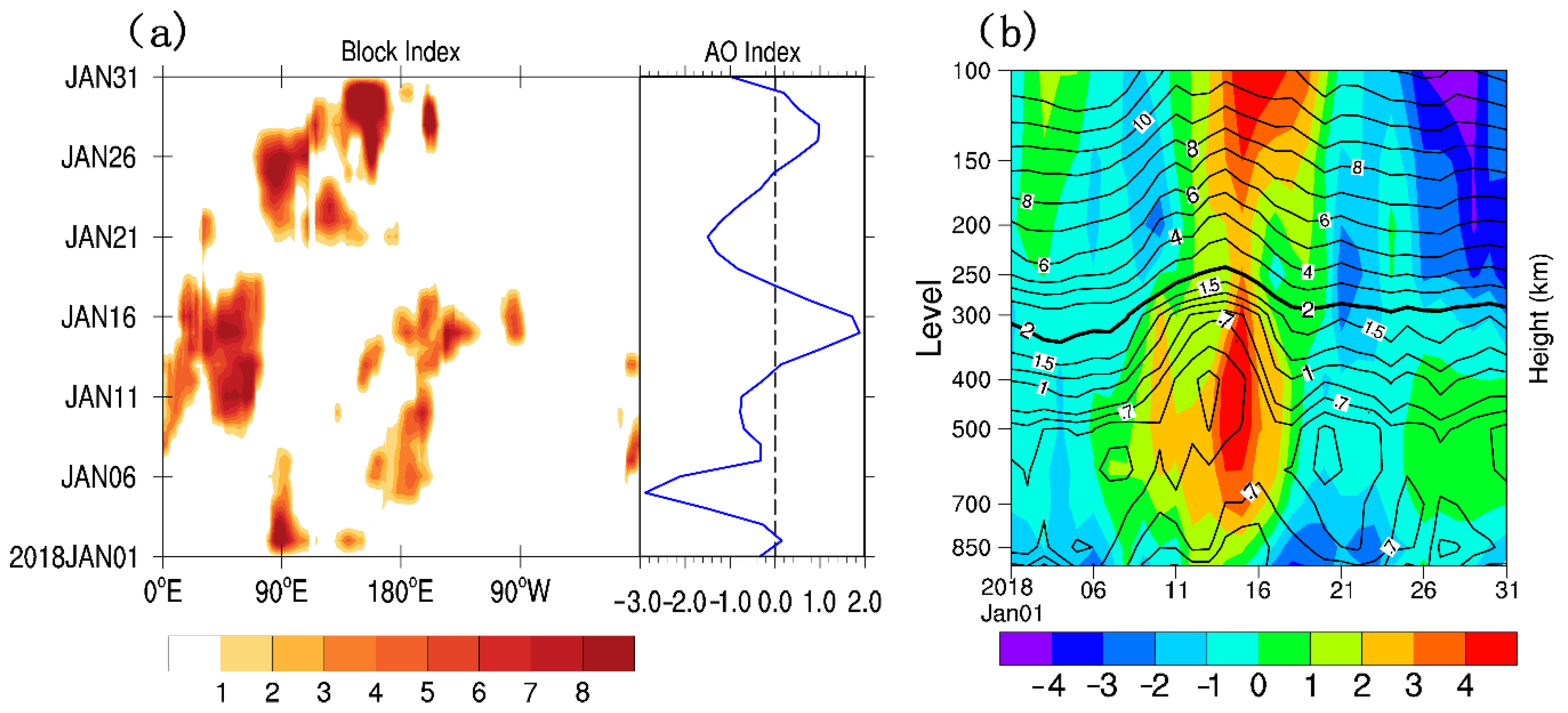
Further exploring the mechanism of how the blocking synergy affects the cold surge, the blocking index (Figure 7a), which can better reveal the dynamic and thermodynamic essence of blocking, shows that there was a clear synergy between European blocking and North American blocking in mid-January. In January 11–17, two blocking ridges combined to strengthen in Europe, and at the same time, the Pacific East-North American blocking ridge was also developing. Double blocking synergy appeared on the 14th and double blocking further strengthened northward on the 15th when large amounts of warm, moist air in the Atlantic and Pacific Ocean were transported to the Arctic, corresponding to the AO phase falling from the positive peak. The double blocking synergy disappeared on the 18th and the accompanying AO turned negative. This synergistic effect well explains the dramatic changes in the AO phase before the cold surge.

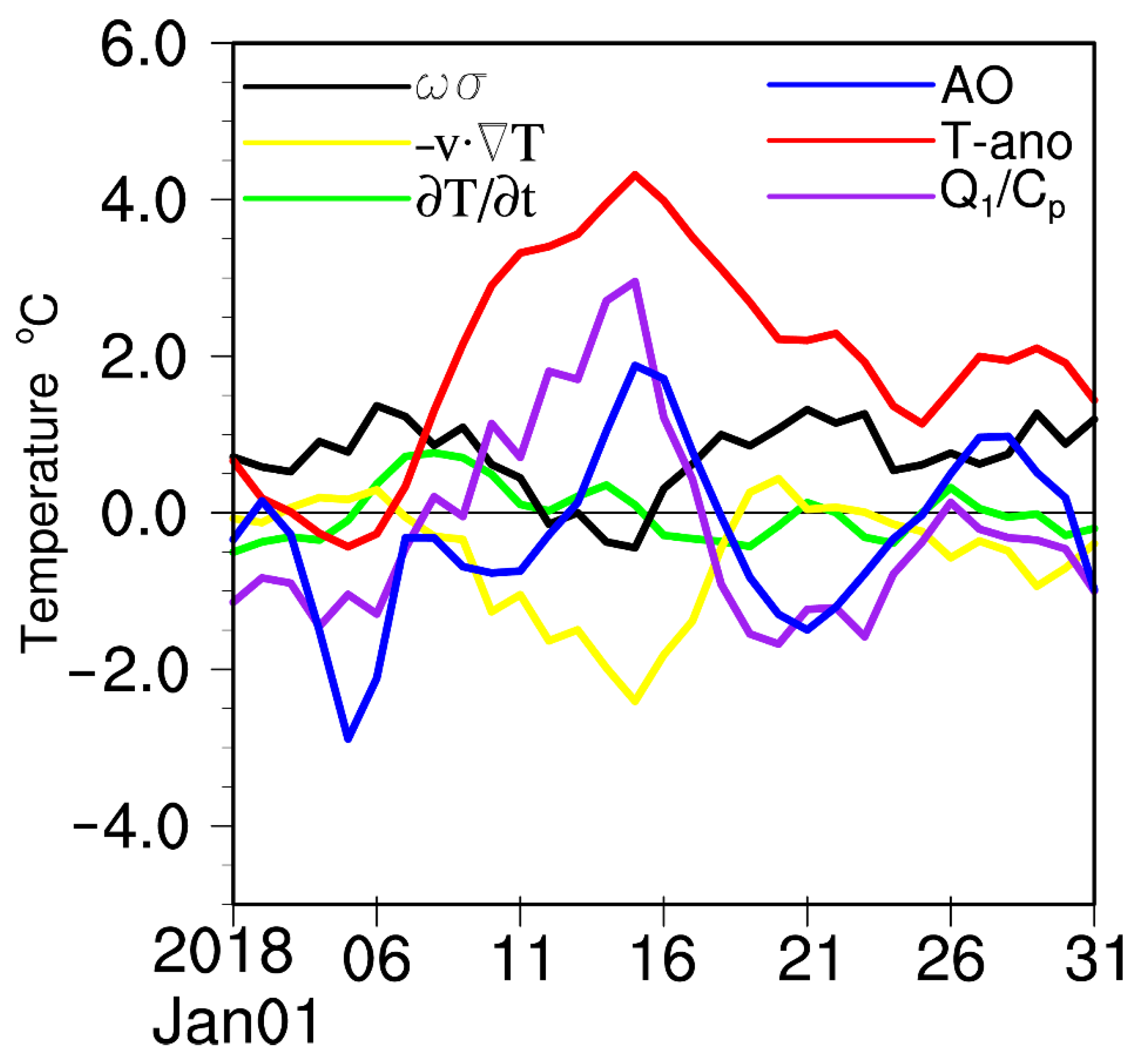
The time-height field of the diabatic heating in the Arctic (67–90° N) and the high latitude (0–70° E, 67–90° N) PV in Europe in January 2018 shows that the largest period of Arctic diabatic heating coincides with the blocking synergy period and on the 15th, the diabatic heating maximum center appeared in the troposphere above the Arctic (Figure 7b). According to the equation of potential vorticity [28,43], due to the effect of diabatic heating, the PV above the heat source decreases (the tropospheric PV contours upwardly bump) and PV below the heat source increases, which causes the polar vortex to weaken. In addition, calculating the magnitude of an individual term of the temperature diagnostic equation (Equation (3)), it was found that diabatic heating contributes the most to Arctic warming during blocking synergy (Figure 8). It can be seen that the change of AO phase is largely affected by the double blocking synergy and diabatic heating.

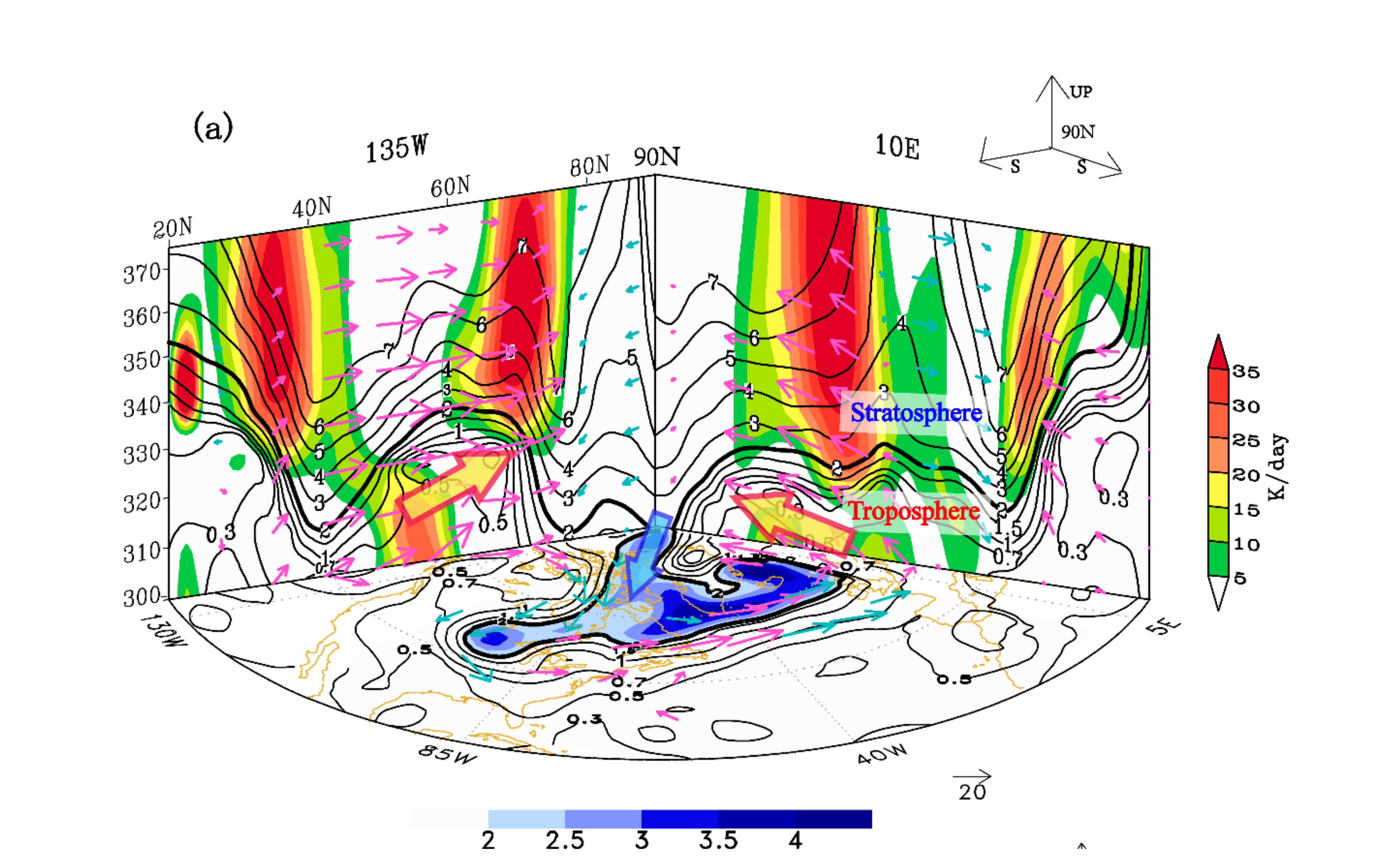
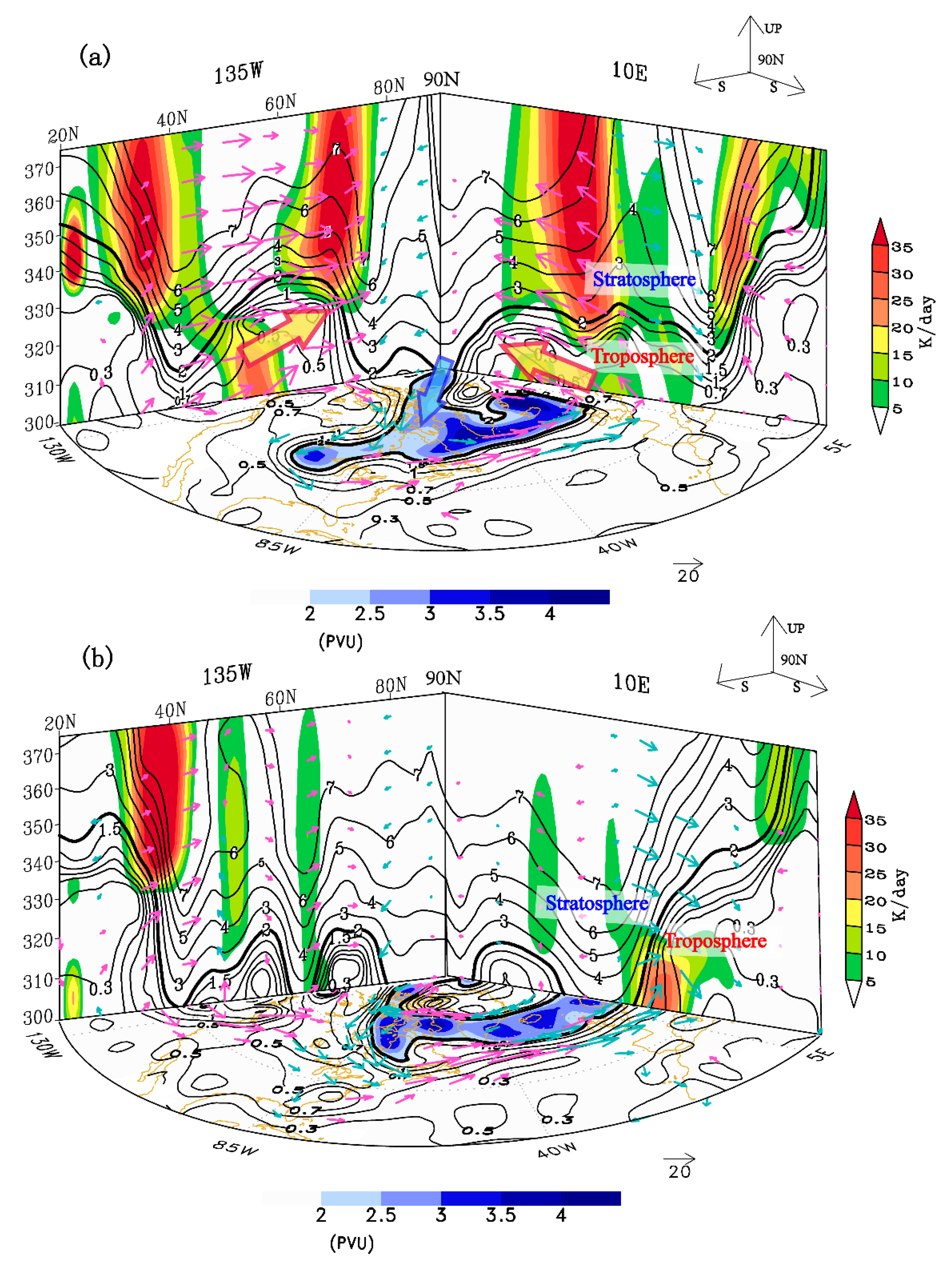
In order to more clearly analyze the influence of the double blocking synergy on the atmospheric circulation and the AO phase transformation, Figure 9 shows three-dimensional maps of the double blocking invading the Arctic on January 15th with the maximum AO index and on the 18th with an AO index close to zero. Figure 9a shows the two strong blockings (low PV) in the Western Europe (10° E) and the Western North America (135° W) simultaneously stretched from mid latitude to Arctic. Above the two blockings, two large diabatic heating zones tilted northward with southerlies, resulting in a PV above and in the north of the heat source decreasing and below the heat source increasing [28,43]. This caused the two ridges that developed northward and upward and further squeezed the high PV cold air of the polar vortex. Under the influence of the double blocking synergy, the high PV was firstly concentrated over the polar region. Therefore, the AO index reached a maximum value on January 15th. Then, a portion in the lower level was squeezed to the east of North America and near Greenland. On January 18th (Figure 9b), as the double blocking deeply stretched to the Arctic accompanied with the diabatic heating rapidly increasing there, the polar high PV cold air was squeezed out of the Arctic, the polar PV contours became relatively flat and the polar vortex became weaker and was split into two parts, as shown in Figure 5. Negative PV more greatly took up the Arctic region. Consequently, the AO index rapidly decreased and turned negative on the 18th.

4. Conclusions and Discussion

The climatic factors and attribution analysis affecting the winter “warm Arctic-Cold Eurasian” modality have been studied by a large number of scholars [6,20,44,45,46,47]. However, impact factors in the extended range of cold extremes have been less explored. This paper uses the PV tool to diagnose and catch the early mid-high-latitude signals of the persistent cold surge in January 2018 and analyze the cause of the AO phase rapid transition before the strongly cold surge. The major findings are summarized below:

(1)

Before the outbreak of the cold surge, high PV cold air successively accumulated in the north-western part of Lake Baikal (80–120° E, 50–70° N); this accumulation made the temperature drop continuously beyond 30 °C, the lowest being −41 °C, forming a direct source of cold air in the East Asian cold surge and directly affecting the intensity of southward cold air.

(2)

The long-term accumulation of cold air on the north-west side of Lake Baikal is the direct reason for the formation of a strong cold surge. Another reason may have been that both a stable north-south exchange resulting from the double blocking synergy in mid-January and then an interception effect resulting from a zonal trough on cold air on the north of a separated low-PV anticyclone had an important impact on the successive accumulation of cold air in the West Siberian Plain.

(3)

Due to the influence of the strong cold surge in North America during the early period (early January), the Atlantic mid-latitude anticyclone rapidly moved eastward and connected with the Western Europe blocking, which is an important reason for the formation of the Atlantic-European poleward transport channel of warm and moist air. This is a key early signal, which occurs on the PV, leading to the coldest day in about 18 days.

(4)

A synergistical poleward development of the Western Europe blocking and the North American blocking is an important reason and early signal of polar vortex splitting and AO phase transition. This phenomenon is like an accelerator which rapidly changes the mid-high latitude synoptic situation but to move less in itself. During the double blocking synergy, a large amount of moist air was transported from the Atlantic and the Pacific Ocean to the Arctic so that the two blockings developed further and the polar vortex weakened under the predominance of diabatic heating. Then, with a split of the polar vortex, the cold air broke southward and AO index dropped rapidly and turned negative.

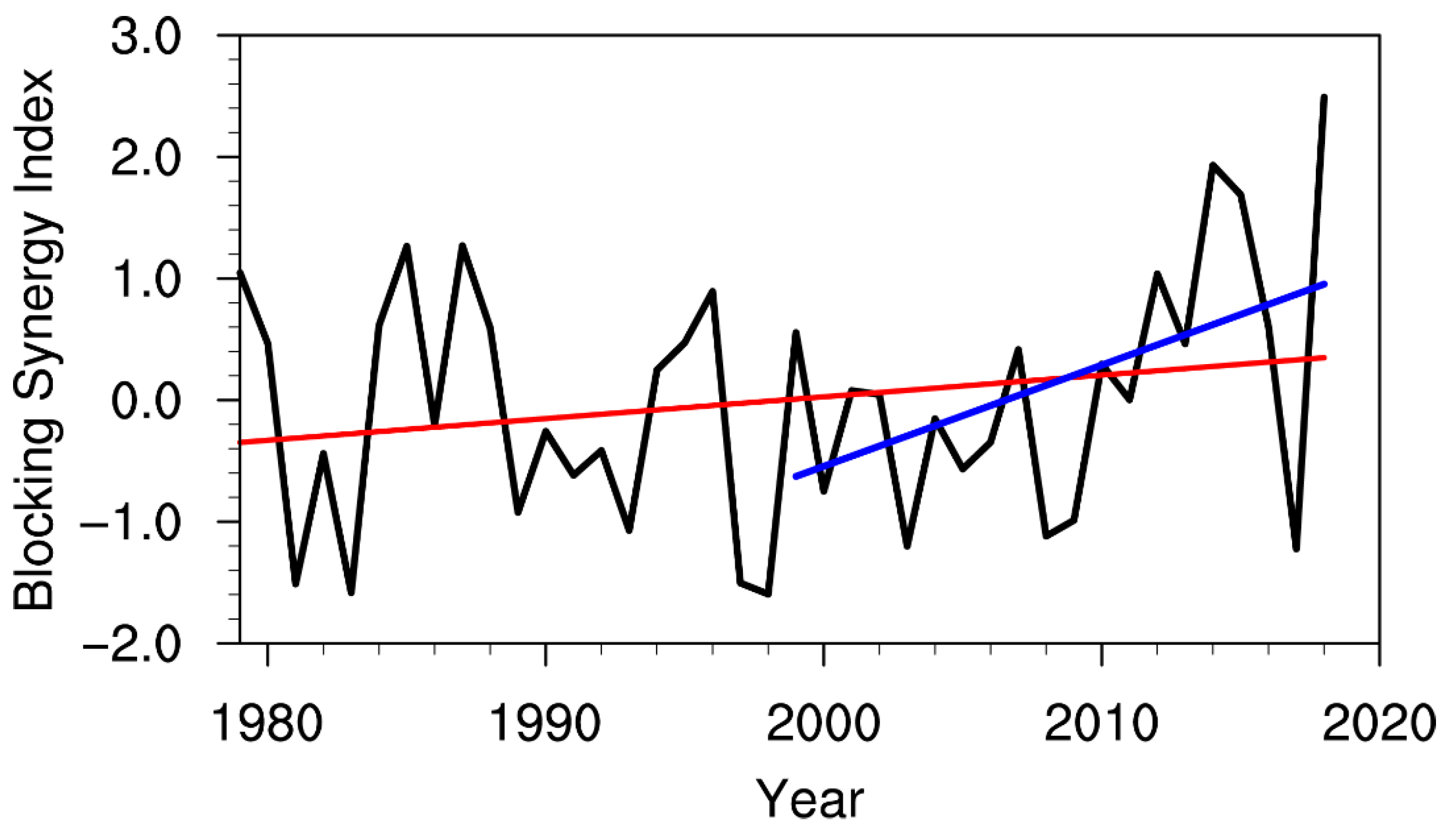
Previous studies about cold surge often focused on the Ural blocking [20,21,22,45,48]. We are looking for more early signals and found that the double blocking synergy is likely responsible for the rapid change in circulation over the polar region and the intense outbreak of Arctic cold air. It is also an early precursor of the extremely persistent cold event over East Asia in late January 2018. Moreover, we think that the blockings stretching into the Arctic Circle likely more largely influence the Arctic circulation systems than those outside the Arctic Circle. According to Equation (2), we thus pick out the blockings into the Arctic Circle by fixing 66° N as the central blocking latitude ${\varphi }_c(\lambda )$. A blocking stretching into the Arctic Circle is detected if $B>0$ at longitude $\lambda$. Then, the $\mathrm{P}\mathrm{V}-\theta$ blocking index averaged over the two regions, the Atlantic-Western Europe (from 40° W to 40° E) and the Pacific-North America (from 90° W to 170° W), could characterize the synergistic effect of the blockings reaching the Arctic. Figure 10 shows that the standardized synergy index of blockings reaching the Arctic Circle has slowly increased since 1979 and rapidly increased since 1999. Moreover, the variance from 1979 to 1998 is 0.961; the variance from 1999 to 2018 is 1.088. The above results show that the blocking synergy is more frequent and drastic. Notably, the blocking synergy index in mid-January 2018 reached the maximum after 1979. More blockings simultaneously reaching the Arctic cause excessive exchanges between mid-latitudes and the Arctic, which is conducive to extreme cold events in the mid-latitudes in winter.

References

- Screen, J.A.; Simmonds, I. The central role of diminishing sea ice in recent Arctic temperature amplification. Nature 2010, 464, 1334–1337. [Google Scholar] [CrossRef] [Green Version]
- Kwok, R.; Rothrock, D.A. Decline in Arctic sea ice thickness from submarine and ICESat records: 1958–2008. Geophys. Res. Lett. 2009, 36, L15501. [Google Scholar] [CrossRef] [Green Version]
- Overland, J.E.; Wang, M.; Walsh, J.E.; Stroeve, J.C. Future Arctic climate changes: Adaptation and mitigation time scales. Earth’s Future 2014, 2, 68–74. [Google Scholar] [CrossRef]
- Cholaw, B.; Jingbei, P.; Zuowei, X.; Liren, J. Recent progresses on the studies of wintertime extensive and persistent extreme cold events in China and large-scale tilted ridges and troughs over the Eurasian continent Chinese. J. Atmos. Sci. 2018, 42, 656–676. (In Chinese) [Google Scholar]
- Johnson, N.C.; Xie, S.P.; Kosaka, Y.; Li, X. Increasing occurrence of cold and warm extremes during the recent global warming slowdown. Nat. Commun. 2018, 9, 1724. [Google Scholar] [CrossRef] [Green Version]
- Cohen, J.; Screen, J.A.; Furtado, J.C.; Barlow, M.; Whittleston, D.; Coumou, D.; Jones, J. Recent arctic amplification and extreme mid-latitude weather. Nat. Geosci. 2014, 7, 627–637. [Google Scholar] [CrossRef] [Green Version]
- Cohen, J.; Barlow, M.; Kushner, P.J.; Saito, K. Stratosphere–troposphere coupling and links with Eurasian land surface variability. J. Clim. 2007, 20, 5335–5343. [Google Scholar] [CrossRef]
- Cohen, J.; Jones, J. A new index for more accurate winter predictions. Geophys. Res. Lett. 2011, 38, 759–775. [Google Scholar] [CrossRef] [Green Version]
- Stroeve, J.C.; Maslanik, J.; Serreze, M.C.; Rigor, I.; Meier, W.; Fowler, C. Sea ice response to an extreme negative phase of the Arctic Oscillation during winter 2009/2010. Geophys. Res. Lett. 2011, 38, L02502. [Google Scholar] [CrossRef]
- Francis, J.A.; Chan, W.; Leathers, D.J.; Miller, J.R.; Veron, D.E. Winter northern hemisphere weather patterns remember summer Arctic sea-ice extent. Geophys. Res. Lett. 2009, 36, L07503. [Google Scholar] [CrossRef] [Green Version]
- Tang, Q.; Zhang, X.; Yang, X.; Francis, J.A. Cold winter extremes in northern continents linked to Arctic sea ice loss. Environ. Res. Lett. 2013, 8, 014036. [Google Scholar] [CrossRef]
- Ding, Q.; Schweiger, A.; L’Heureux, M.; Battisti, D.S.; Po-Chedley, S.; Johnson, N.C.; Steig, E.J. Influence of high-latitude atmospheric circulation changes on summertime Arctic sea ice. Nat. Clim. 2017, 7, 289–295. [Google Scholar] [CrossRef]
- Ma, S.; Zhu, C.; Liu, B.; Zhou, T.; Ding, Y.; Orsolini, Y.J. Polarized response of East Asian winter temperature extremes in the era of Arctic warming. J. Clim. 2018, 31, 5543–5557. [Google Scholar] [CrossRef]
- Gramling, C. Arctic impact. Science 2015, 347, 818–821. [Google Scholar] [CrossRef]
- Francis, J.A.; Vavrus, S.J. Evidence linking Arctic amplification to extreme weather in mid-latitudes. Geophys. Res. Lett. 2012, 39, L06801. [Google Scholar] [CrossRef]
- Ding, Q.; Wallace, J.M.; Battisti, D.S.; Steig, E.J.; Gallant, A.J.; Kim, H.J.; Geng, L. Tropical forcing of the recent rapid Arctic warming in northeastern Canada and Greenland. Nature 2014, 509, 209–212. [Google Scholar] [CrossRef]
- Cohen, J.L.; Furtado, J.C.; Barlow, M.A.; Alexeev, V.A.; Cherry, J.E. Arctic warming, increasing snow cover and widespread boreal winter cooling. Environ. Res. Lett. 2012, 7, 014007. [Google Scholar] [CrossRef]
- Zhao, L.; Zhu, Y.; Liu, H.; Liu, Z.; Liu, Y.; Li, X.; Chen, Z. A stable snow–atmosphere coupled mode. Clim. Dyn. 2016, 47, 2085–2104. [Google Scholar] [CrossRef]
- Pithan, F.; Svensson, G.; Caballero, R.; Chechin, D.; Cronin, T.W.; Ekman, A.M.; Wendisch, M. Role of air-mass transformations in exchange between the Arctic and mid-latitudes. Nat. Geosci. 2018, 11, 805–812. [Google Scholar] [CrossRef]
- Luo, D.; Chen, X.; Dai, A.; Simmonds, I. Changes in atmospheric blocking circulations linked with winter Arctic warming: A new perspective. J. Clim. 2018, 31, 7661–7678. [Google Scholar] [CrossRef]
- Yao, Y.; Luo, D.; Dai, A.; Simmonds, I. Increased quasi stationarity and persistence of winter Ural blocking and Eurasian extreme cold events in response to Arctic warming. Part I: Insights from observational analyses. J. Clim. 2017, 30, 3549–3568. [Google Scholar] [CrossRef]
- Luo, D.; Yao, Y.; Dai, A.; Simmonds, I.; Zhong, L. Increased quasi stationarity and persistence of winter Ural blocking and Eurasian extreme cold events in response to Arctic warming. Part II: A theoretical explanation. J. Clim. 2017, 30, 3569–3587. [Google Scholar] [CrossRef]
- Heo, J.W.; Ho, C.H.; Park, T.W.; Choi, W.; Jeong, J.H.; Kim, J. Changes in Cold Surge Occurrence over East Asia in the Future: Role of Thermal Structure. Atmosphere 2018, 9, 222. [Google Scholar] [CrossRef] [Green Version]
- Ding, Y.; Ma, X. Analysis of isentropic potential vorticity for a strong cold wave in 2004/2005 winter. Acta Meteorol. Sin. 2007, 65, 695–707. (In Chinese) [Google Scholar]
- Wu, B.Y. Two extremely cold events in East Asia in January of 2012 and 2016 and their possible associations with Arctic warming. Trans. Atmos. Sci. 2019, 42, 14–27. (In Chinese) [Google Scholar]
- Dee, D.P.; Uppala, S.M.; Simmons, A.J.; Berrisford, P.; Poli, P.; Kobayashi, S.; Bechtold, P. The ERA-Interim reanalysis: Configuration and performance of the data assimilation system. Quart. J. Roy. Meteor. Soc. 2011, 137, 553–597. [Google Scholar] [CrossRef]
- Kalnay, E.; Kanamitsu, M.; Kistler, R.; Collins, W.; Deaven, D.; Gandin, L.; Zhu, Y. The NCEP/NCAR 40-year reanalysis project. Bull. Am. Meteorol. Soc. 1996, 77, 437–472. [Google Scholar] [CrossRef] [Green Version]
- Hoskins, B.J.; McIntyre, M.E.; Robertson, A.W. On the use and significance of isentropic potential vorticity maps. Quart. J. Roy. Meteor. Soc. 1985, 111, 877–946. [Google Scholar] [CrossRef]
- Pelly, J.L.; Hoskins, B.J. A new perspective on blocking. J. Atmos. Sci. 2003, 60, 743–755. [Google Scholar] [CrossRef]
- Yanai, M.; Esbensen, S.; Chu, J.H. Determination of bulk properties of tropical cloud clusters from large-scale heat and moisture budgets. J. Atmos. Sci. 1973, 30, 611–627. [Google Scholar] [CrossRef]
- Hsu, P.C.; Lee, J.Y.; Ha, K.J.; Tsou, C.H. Influences of boreal summer intraseasonal oscillation on heat waves in monsoon Asia. J. Clim. 2017, 30, 7191–7211. [Google Scholar] [CrossRef]
- Liess, S.; Agrawal, S.; Chatterjee, S.; Kumar, V. A teleconnection between the West Siberian Plain and the ENSO region. J. Clim. 2017, 30, 301–315. [Google Scholar] [CrossRef] [Green Version]
- Cai, M.; Shin, C. A total flow perspective of atmospheric mass and angular momentum circulations: Boreal winter mean state. J. Atmos. Sci. 2014, 71, 2244–2263. [Google Scholar] [CrossRef]
- Kanno, Y.; Abdillah, M.R.; Iwasaki, T. Charge and discharge of polar cold air mass in northern hemispheric winter. Geophys. Res. Lett. 2015, 42, 7187–7193. [Google Scholar] [CrossRef]
- Yu, Y.-Y.; Cai, M.; Ren, R.-C.; van den Dool, H.M. Relationship between warm airmass transport into upper polar atmosphere and cold air outbreaks in winter. J. Atmos. Sci. 2015, 72, 349–368. [Google Scholar] [CrossRef] [Green Version]
- Yu, Y.-Y.; Ren, R.-C.; Cai, M. Dynamical linkage between cold air outbreaks and intensity variations of the meridional mass circulation. J. Atmos. Sci. 2015, 72, 3214–3232. [Google Scholar] [CrossRef]
- Hoskins, B. Potential vorticity and the PV perspective. Adv. Atmos. Sci. 2015, 32, 2–9. [Google Scholar] [CrossRef]
- Zhao, Q. Analysis with isentropic potential vorticity on a cold wave in southeastern Asia. J. Appl. Meteor. Sci. 1990, 4, 392–399. (In Chinese) [Google Scholar]
- Bi, M.; Ding, Y. A study of budget of potential vorticity of blocking high during the drought period in summer of 1980. J. Appl. Meteor. Sci. 1992, 2, 145–156. (In Chinese) [Google Scholar]
- Zhao, L.; Ding, Y. Sources and transfer of high isentropic potential vorticity during meiyu period. J. Appl. Meteor. Sci. 2008, 19, 697–709. (In Chinese) [Google Scholar]
- Zhao, L.; Ding, Y. Potential vorticity analysis of cold air activities during the East Asian summer monsoon. Chin. J. Atmos. Sci. 2009, 33, 359–374. (In Chinese) [Google Scholar]
- Zhang, C.; Tan, Y.; Li, C.; Ping, Y. Influences of interactions between high-frequency eddies and low-frequency variabilities on the process of Rossby wave breaking. Chin. J. Atmos. Sci. 2019, 43, 221–232. (In Chinese) [Google Scholar]
- Zheng, Y.; Wu, G.; Liu, Y. Dynamical and thermal problems in vortex development and movement. Part I: A. PV-Q. View. Acta Meteor. Sin. 2013, 71, 185–197. (In Chinese) [Google Scholar] [CrossRef]
- Xu, X.; He, S.; Li, F.; Wang, H. Impact of northern Eurasian snow cover in autumn on the warm Arctic–cold Eurasia pattern during the following January and its linkage to stationary planetary waves. Clim. Dyn. 2018, 50, 1993–2006. [Google Scholar] [CrossRef]
- Luo, D.; Xiao, Y.; Yao, Y.; Dai, A.; Simmonds, I.; Franzke, C.L. Impact of Ural blocking on winter warm Arctic–cold Eurasian anomalies. Part I: Blocking-induced amplification. J. Clim. 2016, 29, 3925–3947. [Google Scholar] [CrossRef]
- Luo, D.; Xiao, Y.; Diao, Y.; Dai, A.; Franzke, C.L.; Simmonds, I. Impact of Ural blocking on winter warm Arctic–cold Eurasian anomalies. Part II: The link to the North Atlantic Oscillation. J. Clim. 2016, 29, 3949–3971. [Google Scholar] [CrossRef]
- Luo, D.; Chen, Y.; Dai, A.; Mu, M.; Zhang, R.; Ian, S. Winter Eurasian cooling linked with the Atlantic multidecadal oscillation. Environ. Res. Lett. 2017, 12, 125002. [Google Scholar] [CrossRef] [Green Version]
- Cheung, H.N.; Zhou, W.; Mok, H.Y.; Wu, M.C. Relationship between Ural–Siberian blocking and the East Asian winter monsoon in relation to the Arctic Oscillation and the El Niño–Southern Oscillation. J. Clim. 2012, 25, 4242–4257. [Google Scholar] [CrossRef]
- The China Meteorological Administration, the Surface Temperature Data. Available online: http://data.cma.cn/ (accessed on 13 February 2020).
Figure 1.
(a) Time series of the near-surface air temperature anomaly averaged over China for January from 1959 to 2018 using gauged data (red curve with hollow circle; units: °C; the green and black straight lines are the trend lines of recent 18 years (−0.012 °C /year) and 60 years (0.023 °C /year), respectively; the horizontal dashed line is −1.42 °C, corresponding to a −1.25 standard deviation threshold). (b) Same as (a) but for late (21–31) January. The trends in the last 18 and 60 years are −0.032 °C /year and 0.012 °C /year, respectively, and the horizontal dashed line is −2.35 °C. (c) Probability density functions (PDFs) of surface temperature anomalies in late January 1959–2018 (the red and blue solid curves are a normal and a generalized extreme value (GEV) fits, respectively). The anomalies are relative to the 1959–2018 mean.
Figure 2.
The maps of the near-surface air temperature anomalies (colored shading; units: °C) over China in early (a), mid (b), late (c) January 2018, relative to 1959–2018. The thick purple lines are 0 °C in climatology (for the period 1959–2018) and the thick green lines are 0 °C in 2018.
Figure 3.
(a) The leading correlation coefficient map when 345 K isentropic PV is 11 days ahead of China’s surface temperature for the period from 1 January to 10 February in 2018 (the contour outlines the significant correlation regions with a 95% confidence level). (b) Leading correlation coefficients between the daily isentropic PV series averaged over the northwestern region of Lake Baikal (80–120° E, 50–70° N) as shown in the box in (a) at 315 K (blue), 330 K (red) and 345 K (green) and the daily mean China near-surface air temperature series for the period from 1 January to 10 February (the thick horizontal black line indicates the 95% confidence level).
Figure 4.
(a) Isentropic surface–time profile of area (60–70° N, 80–100° E) in the high PV source (located on the northwestern side of Lake Baikal (80–120° E, 50–70° N)) in January 2018, overlapped lead and lag correlations. The dot (negative correlation) and the mesh (positive correlation) areas represent significant correlations above a 0.10 significance level. Lead01–27 represents that the PV series lead surface temperature series of China (from 1 January to 9 February) by 1 to 27 days, respectively; lag0–03 represents that the PV lag temperature by 0 to 3 days, respectively. The lowest temperature date, 28 January, is the base date, indicated by the thick red dashed straight line. The thick solid contours in (a) and (b) are 2PVU. (b) Same as (a), but for the 305 K 90° E latitude-time profile. (c) Daily series of surface temperature averaged over China (T) (red curve, units: °C), 305 K PV averaged over the high PV source (80–120° E, 50–70° N) (isentropic PV) (black dotted curve, units: PVU), 1000hPa temperature at the point (60° N, 100° E) (T_Baikal) (purple dotted curve, units: °C) and AO index (blue curve) in January.
Figure 5.
315 K isentropic PV (contour, units: PVU) and wind (arrow, units: m s−1) fields on some given dates in January 2018. The purple and blue arrows represent southerly and northerly, respectively, and wind speed larger than 15 m s−1. PV in the blue shade is greater than 4 PVU; PV less than 2 PVU in the north of 50° N is marked in red. The thick solid contours are 2 PVU.
Figure 6.
(a) Thirteen and (b) 14 January 2018, longitude-height profiles of PV (contours), wind (vectors) along latitudes (50–55° N) and diabatic heating along latitudes (50–60° N) (shading, units: K day−1). The red thick solid contours are 0.8 PVU. The black thick solid contours are 2 PVU. The arrows are vector wind field from composites of the zonal wind (units: m s−1) and the vertical velocity of p-coordinate system (units: −100×Pa s−1): blue indicates easterly and red indicates westerly.
Figure 7.
On January 2018 (a) blocking index (left panel) and AO index (right panel); (b) diabatic heating in the Arctic (67–90° N) (shading, units: K day−1) and the PV in Eurasian polar region (0–70° E, 70–90° N) (contours, units: PVU).
Figure 8.
Different items of the temperature diagnostic equation, AO index and mean temperature anomaly between 1000 and 300hPa averaged over the Arctic (67°–90° N). The blue curve shows the AO index, red is the Arctic temperature anomaly, purple is the diabatic heating (), black is the convection item (), yellow is the advection term (), and green is the local variation of temperature ().
Figure 9.
The three-dimensional map of PV (contours, thickened black contours of 2 PVU represent the dynamic tropopause), diabatic heating (red-yellow-green shading in the top two panels) and wind field (the purple and blue arrows indicate southerly and northerly, respectively) between North America and Western Europe on (a) 15 and (b) 18 January 2018: (bottom) 300 K isentropic surface (area with >2 PVU PV is filled with blue shading); (top) latitudinal-isentropic height profiles along 135° W and 10° E.
Figure 10.
Time series of the standardized synergy index of blockings stretching into the Arctic (in the north of 66° N) for mid-January from 1979 to 2018. The red straight line is the trend line of 40 years, 0.018/year; the blue straight line is the trend line of recent 20 years, 0.083/year. See text for the details.
© 2020 by the authors. Licensee MDPI, Basel, Switzerland. This article is an open access article distributed under the terms and conditions of the Creative Commons Attribution (CC BY) license (http://creativecommons.org/licenses/by/4.0/).
Share and Cite
MDPI and ACS Style
Dong, W.; Zhao, L.; Zhou, S.; Shen, X. A Synergistic Effect of Blockings on a Persistent Strong Cold Surge in East Asia in January 2018. Atmosphere 2020, 11, 215. https://0-doi-org.brum.beds.ac.uk/10.3390/atmos11020215
AMA Style
Dong W, Zhao L, Zhou S, Shen X. A Synergistic Effect of Blockings on a Persistent Strong Cold Surge in East Asia in January 2018. Atmosphere. 2020; 11(2):215. https://0-doi-org.brum.beds.ac.uk/10.3390/atmos11020215
Chicago/Turabian StyleDong, Wei, Liang Zhao, Shunwu Zhou, and Xinyong Shen. 2020. "A Synergistic Effect of Blockings on a Persistent Strong Cold Surge in East Asia in January 2018" Atmosphere 11, no. 2: 215. https://0-doi-org.brum.beds.ac.uk/10.3390/atmos11020215
Note that from the first issue of 2016, this journal uses article numbers instead of page numbers. See further details here.