LES Simulation of Wind-Driven Wildfire Interaction with Idealized Structures in the Wildland-Urban Interface


1
School of Mechanical Engineering, University of Tehran, Tehran 14395-515, Iran
2
School of Engineering and Information Technology, UNSW Canberra, Canberra, ACT 2612, Australia
3
School of Science, UNSW Canberra, Canberra, ACT 2612, Australia
*
Authors to whom correspondence should be addressed.
Atmosphere 2021, 12(1), 21; https://0-doi-org.brum.beds.ac.uk/10.3390/atmos12010021
Submission received: 3 December 2020
/
Revised: 16 December 2020
/
Accepted: 23 December 2020
/
Published: 25 December 2020
(This article belongs to the Special Issue Coupled Fire-Atmosphere Simulation)
Abstract
:This paper presents a numerical investigation of the impact of a wind-driven surface fire, comparable to a large wildfire, on an obstacle located downstream of the fire source. The numerical modelling was conducted using FireFOAM, a coupled fire-atmosphere model underpinned by a large eddy simulation (LES) solver, which is based on the Eddy Dissipation Concept (EDC) combustion model and implemented in the OpenFOAM platform (an open source CFD tool). The numerical data were validated using the aerodynamic measurements of a full-scale building model in the absence of fire effects. The results highlighted the physical phenomena contributing to the fire spread pattern and its thermal impact on the building. In addition, frequency analysis of the surface temperature fluctuations ahead of the fire front showed that the presence of a building influences the growth and formation of buoyant instabilities, which directly affect the behaviour of the fire’s plume. The coupled fire-atmosphere modelling presented here constitutes a fundamental step towards better understanding the behaviour and potential impacts of large wind-driven wildland fires in wildland-urban interface (WUI) areas.
1. Introduction
Wildfires are a major natural hazard, which can have disastrous consequences from socio-economic and environmental points of view. Given the apparent increase in large wildfires [1] and continued urban expansion into wildland areas [2], there is a clear need for further study of the vulnerability of built assets to fires impacting the wildland-urban interface (WUI). Such studies underpin further development of comprehensive wildfire risk management strategies, including improved urban planning.
Modern Computational Fluid Dynamic codes have played an increasingly important role in understanding the physical processes driving fire behaviour and in improving our ability to predict it. In fact, computational tools are widely used to complement laboratory-scale studies and to compensate for the fact that the results of laboratory-scale studies are difficult to apply directly to large wildfire situations [3]. The first fully physical multiphase wildfire model was developed by Grishin [4]. This model has formed the basis for the development of more advanced, fully physical wildfire models capable of handling additional physicochemical phenomena (e.g., WFDS (Wildland Fire Dynamics Simulator) [5], and FIRETEC code [6]).
Indeed, over the last two decades, significant progress has been made in the development of physics-based wildfire models. Some examples include Meroney et al. [7], who presented a simplified computational model to investigate fire spread within the idealized generic porous models of 3D city structures and Filippi et al. [8,9,10], who proposed an approach to couple a fire area simulator to a mesoscale weather numerical model to simulate local fire/atmosphere interaction. The authors numerically compared the coupled approach between the meso-non-hydrostatic (NH) large eddy simulation (LES) mesoscale atmospheric model and the ForeFire wildland fire area simulator with experimental data to evaluate the performance of the proposed coupled approach in forecasting fine-scale properties of the dynamics of wildland fires.
ForeFire remains a front-tracking model similar to FARSITE, PROMETHEUS, ELMFIRE, etc., where the key principle is to consider a propagating front to represent how the active flame zones propagate over landscapes. This requires a parameterization of the rate of spread, and ForeFire can use either the Rothermel model [11], Finney et al. [12], or the Balbi model [13]. In fact, Rothermel’s model is considered as a semi-empirical rate-of-spread law, while Balbi’s model is considered as a quasi-physical rate-of-spread law. Still, both remain a simplified representation of the reality by using the fire front paradigm.
Generally, fire models range from tools based on the Rothermel model [11], fire spread rate formulas, such as BehavePlus [14] and FARSITE [15], suitable for operational prediction, to sophisticated 3D computational fluid dynamics and combustion simulations appropriate for research and reanalysis, such as FIRETEC and WFDS. PC-based solvers such as BehavePlus predict the fire spread rate at a single point of fuel and a set of environmental data; FARSITE employs the fire spread rate to provide a two-dimensional simulation on a PC; whereas FIRETEC and WFDS need a parallel supercomputer and run a lot slower than real time. Among coupled atmosphere-wildland fire solvers, WRF-Fire [16] consists of a fire-spread model, achieved by the level-set method, coupled with the Weather Research and Forecasting model (WRF). Kochanski et al. [17] evaluated and improved the performance of the coupled atmosphere-fire model WRF-SFIRE and showed WRF-SFIRE is capable of predicting head-fire rate of spread and fire plume vertical temperature up to 10 m above ground level.
Similarly, a series of papers [18,19] outlines the development and application of a numerical physics-based multiphase model called FIRESTAR3D. FIRESTAR3D is a 3D finite volume model based on a fully physical multiphase model to simulate the ignition and propagation of grassland fires, crown fire and wildfires at local scales (<500 m) [18]. The impact of wind velocity and terrain features on large scale fires was extensively studied using FireFOAM in a series of papers [20,21,22]. The authors successfully developed a numerical model to express the dynamic characteristics of the fire in terms of fire-induced pressure and viscous forces.
While full physical (and other) models have been used extensively to gain a better understanding of the fundamental behaviour of wildfires [11,19,23,24,25], mechanisms of fire spread in WUI fires have not received as much research attention and so are not as well-understood. Recently, however, there have been some efforts to study fire configurations that are more relevant to WUI fires. Linn et al. [26] developed a fast-running numerical tool based on integration of a phenomenologically-based fire spread model with a fast-running atmospheric solver initially designed for application to urban environments. This tool allowed for more computationally efficient accounting of fire-atmospheric feedbacks and provides fire planners with the opportunity to compare, assess, and design prescribed burn plans to assist with WUI fire management more rapidly. Despite its relative simplicity, this model showed a similar capability to capture the underlying physics and basic trends in fire behaviour to more sophisticated models such as FIRETEC.
Hilton et al. [27] presented a novel low-fidelity numerical model for the calculation of radiative heat flux loadings on buildings in the WUI and demonstrated its utility in risk assessment of infrastructure in areas impacted by wildfires. The evolution of the fire front in this approach was simulated using a quasi-steady model for the fire’s rate of spread, which means that it does not properly account for dynamic fire behaviour and fire-atmosphere interactions. Similarly, Cohen [28] proposed a theoretical model based on ideal heat transfer characteristics to investigate direct flame heating leading to building ignition during wildland fires. This study also determined the critical flame-to-structure distance, at which wooden walls would readily ignite. Mell et al. [29] conducted a comprehensive review of approaches commonly used for addressing problems concerning WUI fires. They concluded that physics-based modelling approaches can be reliably used to determine structure exposure conditions, and to develop new building test methods and standards.
A detailed numerical study based on a fully physical model (Fire Dynamic Simulator, or FDS) focusing on the effect of wind-driven fires on a building was first carried out by He et al. [30]. The numerical model was validated in the absence of fire using mean pressure measurements made on the full-scale, cube-shaped Silsoe building [31]. It is worth mentioning that the Silsoe experiment was carried out in idealized situations (e.g., cubic building, flat terrain) and provides a set of important benchmark data about the fundamental aerodynamic behaviour of low-rise buildings under wind loads. Several attempts have also been made to predict high-risk areas in the WUI using high-fidelity physics-based CFD models. Fryanova et al. [32] used WFDS to study the effects of fire intensity and wind speed on the likelihood of structure ignition. A crown fire was represented as an equivalent heat and mass source at an appropriate height, and the resulting hydrodynamic and thermal interactions between the plume and wind flow were analysed to assess the possibility of ignition of buildings. Similarly, Pimont et al. [33] used FIRETEC to investigate the minimal “clearing” distance required between buildings and forest in WUI areas to maintain safe working zones for firefighters and to minimize the chance of structure ignition. They found that a clearing distance of 50 m is an acceptable threshold for both materials and firefighters for both thermal radiation and gas temperature.
Understanding flow pattern due to freestream velocity variation associated with the interaction of fire and cross-wind flow around the building, and also variation of the structure’s surface temperature due to radiative heat flux, are of great importance [34,35] because the consequences may have major implications in building design against wildland fire attacks [36,37,38]. However, a fundamental understanding of how the interaction of fire and wind can alter the time-dependent flow patterns of velocity variation and the surface temperature of the building has remained elusive.
In the CFD approach, the fire behaviour could be modelled through the computation of algebraic equations arising from fundamental physical laws and constitutive equations to accurately model fire and its impact on structure, properties and so on.
This study explores the fundamental mechanisms of how the interaction of horizontal cross wind flow with a vertical plume alters the velocity profile around the building and the surface temperature of the building downstream of the fire source. FireFOAM was used as a CFD solver in this study. This solver is a derivative of the OpenFOAM [39] platform, specifically designed for fire dynamic simulations. FireFOAM is a large eddy simulation (LES) fire dynamics transient solver for large-scale fires and turbulent diffusion flames with reacting particle clouds, surface film and pyrolysis modelling. Despite its capability in large-scale fire dynamic modelling, it has not yet been employed in wind-driven wildfire-urban interface simulations, hence this study aimed to provide further fundamental insights into the interaction between a wind-driven fire and a building, thereby improving our understanding of the mechanisms involved in fire propagation and structure loss in WUI areas using FireFOAM code. The code is used to investigate the thermal loading on a building exposed to a wildfire that is encroaching on the wildland-urban interface. Dynamic fire behaviour is also discussed, and observations of the flame structure are described. The present study provides valuable information relevant to the identification of sources for structure ignition, enhanced turbulence (important for ember generation, transport and accumulation) and strong winds/pressure gradients that could affect the integrity of structures, allowing for greater ember incursion and other damage. Indeed, it is worth noting that the effect of strong pyrogenic winds is not generally considered as part of existing risk management doctrine (including building standards, asset protection zones (APZs), etc.).
2. Model Description
In the present paper, a 6 × 6 × 6 m cube is used to represent an idealized building impacted by a wind-driven wildfire. The geometric dimensions are the same as those used in the full-scale Silsoe cube experiment [31]. The cubic building is surrounded by a 50 × 30 × 25 m computational domain as illustrated in Figure 1. According to the recommendations made by Richards and Norris [40], the domain boundaries in this configuration are far enough from the building to minimize adverse boundary condition effects. A fire source running across the entire domain was placed 20 m upstream of the building to mimic a line fire configuration. Methane with a fixed mass flow rate corresponding to a specified heat release rate (HRR) of 180 MW was selected as the fuel source. In the wildfire literature, it is more common to use fire line intensity instead of HRR [41]. As such, in this study we consider a fire with a fixed fire line intensity of 6 MW/m, equivalent to a typical wildfire scenario involving a fire propagating with a rate of spread of 0.75 m/s through a fuel load of 0.4 kg/m2, which represents “average” grassland fuels.
A power-law inflow velocity profile based on Equation (1) was imposed at the domain inlet. Random noise was also superimposed with the mean velocity to reconstruct the turbulent fluctuations.
To lower the cost linked with simulation of the transition process, simulation of spatially evolving turbulence begins with an inflow boundary that is shifted in a shorter distance upstream of the domain of interest [42]. In an ideal situation, having adequately precise inflow conditions at this boundary that result in a more realistic turbulent boundary layer with accurate skin friction is obtained within a short distance downstream. However, practically this is not usually feasible, and the inflow boundary might have to be moved further upstream to let error relaxation assist in estimating the inflow conditions. Having such a “development section” increases the overall cost of the simulations [42]. One simple and yet effective method to specify turbulent inflow conditions and to minimize the cost associated with generating the inflow data is to superpose random fluctuations on a desired mean velocity profile [43]. Despite its simplicity, the random fluctuation approach to introduce perturbations to the flow has been used with varying degrees of success [44,45].
In Equation (1), Zref is the reference height, which is taken as equal to the building’s height (6 m) and Uref is the reference velocity equal to 6 m/s. The exponent is a function of terrain characteristics and is assumed to be 0.16 in the present study based on the terrain category of the experiment site [46]. A typical atmospheric pressure condition (free inflow/outflow at atmospheric pressure) was applied for the top and outlet boundaries, while the side boundaries were treated as free slip boundaries. A wall model as suggested by Launder and Spalding [47] was applied for the near-wall treatment of turbulent flow. This self-adapting wall function allows direct resolution of the near-wall eddies for a fine wall grid corresponding to the dimensionless wall distance parameter of less than 5 (i.e., in the case of y+ < 5 m, the turbulent boundary layer is fully resolved up to viscous sublayer). It should be noted that y+ is a dimensionless parameter representing the first cell size near the wall. Further information regarding the y+ criterion can be found in [48]. For more information regarding implementation of boundary conditions, readers are referred to [19,49].
A high-quality grid was generated using successive zonal refinement. Following this strategy, a subdomain of size 22 × 20 × 12 m was defined around the building to ensure that the complex vortical flow structures formed behind the building were captured accurately (see Figure 1). The second level of grid refinement was set to resolve the near-wall regions around the building. In addition, a spanwise refinement was defined throughout the entire domain providing a high-resolution mesh near the floor. Further information on the grid characteristics will be given in the following section.
2.1. Mathematical and Numerical Modelling
Numerical simulations were conducted using FireFOAM [50], which is a powerful large eddy simulation (LES)-based finite volume solver that is available as a C++ library in the OpenFOAM CFD package. FireFOAM incorporates a number of efficient CFD submodels to describe processes such as radiant heating, pyrolysis, combustion and turbulence. It has been successfully used in many practical applications such as solid fuel pyrolysis [51], fire suppression [52] and fire-wall interaction [53]. FireFOAM has also been demonstrated to be an effective tool in wildfire modelling [25]. The Favre-filtered formulation of the fully compressible Navier-Stokes equations representing the fire dynamics in the most common form is written as a set of conservation equations of mass, momentum, energy and chemical species mass fraction. A reduced single-step combustion composed of the components has been assumed (CH4 + 2O2 + 7.5N2 → CO2 + 2H2O + 7.5N2 [54]).
In these equations, , p, u, , Y and Sct are the density, pressure, velocity, sensible enthalpy, mass fraction and turbulent Schmidt number, respectively. The symbols − and ~ denote spatial and Favre filtering [55], respectively. is the total radiative heat flux (W/m2) of the gas mixture. is the heat generated by combustion and is expressed as the reaction rate of fuel multiplied by the heat of combustion:
Finally, Jk in Equation (4) denotes the mass-diffusive flux accounting for the Soret effect (thermodiffusion) and is calculated using Hirschfelder-Curtiss correlation [56], in which both advective and diffusive mass fluxes are taken into consideration. This avoids possible underestimation error in the mass flow rate calculation at the inlet fuel boundary [50]. The mass diffusion coefficient for each component is written as
It should be noted that the mass diffusion coefficients, Dk, were assumed to be constant and written as a function of the corresponding Schmidt number, Sck. The values of the Schmidt number for all components in the methane combustion process are reported in [57]. In the present LES approach, the wall-adapting local eddy (WALE)-viscosity method was employed for subgrid scale (SGS) modelling. This method has shown remarkable results, particularly in wall-bounded flows [58]. According to this model, the SGS kinetic energy, SGS viscosity and corresponding turbulent mixing time are defined as follows:
where is the rate of strain tensor, is a special tensor defined in [58], and are the model constants, ∆ is the filter width and is a specific form of the rotation rate tensor [58]. The well-established eddy dissipation concept (EDC) [59] was applied for combustion modelling. The EDC model has shown great superiority in modelling well-ventilated diffusion flames [50]. In the EDC, the combustion is controlled by turbulent mixing assuming infinitely fast reaction kinetics. Thus, the fuel mass reaction rate, , is calculated as
where is the model coefficient with a default value of 4 and is the mixing time-scale. and rs are the fuel mass fraction, the oxygen mass fraction, and the stoichiometric oxygen-to-fuel mass ratio, respectively.
Radiation modelling was conducted using the finite volume discrete ordinate method (fvDOM) [50]. To solve the radiative transfer equation (RTE) accurately, 64 solid angles were used for angular discretization. In addition, the weighted-sum-of-grey-gases model (WSGGM) was used to calculate absorption/emission coefficients [60].
A fully implicit second-order Gauss linear scheme was used in space while a first-order Euler method was used as the temporal scheme. FireFOAM takes advantage of the PIMPLE algorithm for pressure-velocity coupling [61]. Making use of a SIMPLE iteration loop embedded in a PISO (Pressure-Implicit with Splitting of Operators) algorithm, the PIMPLE algorithm ensures numerical stability with large Courant numbers (i.e., CFL = U∆t/∆x). This is found to be of significant importance in LES calculations where the grid resolution is high and local Courant numbers might exceed the stability limit (CFL = 1). In the current study, 5 iterations in the outer SIMPLE loop plus 2 iterations over the inner PISO loop (with pressure correction) are considered to ensure the required level of numerical convergence. In addition, the convergence criterion is met when the L2-norms of all transport equation residuals (in normalized form) reach 10−5.
2.2. Computational Model Verification
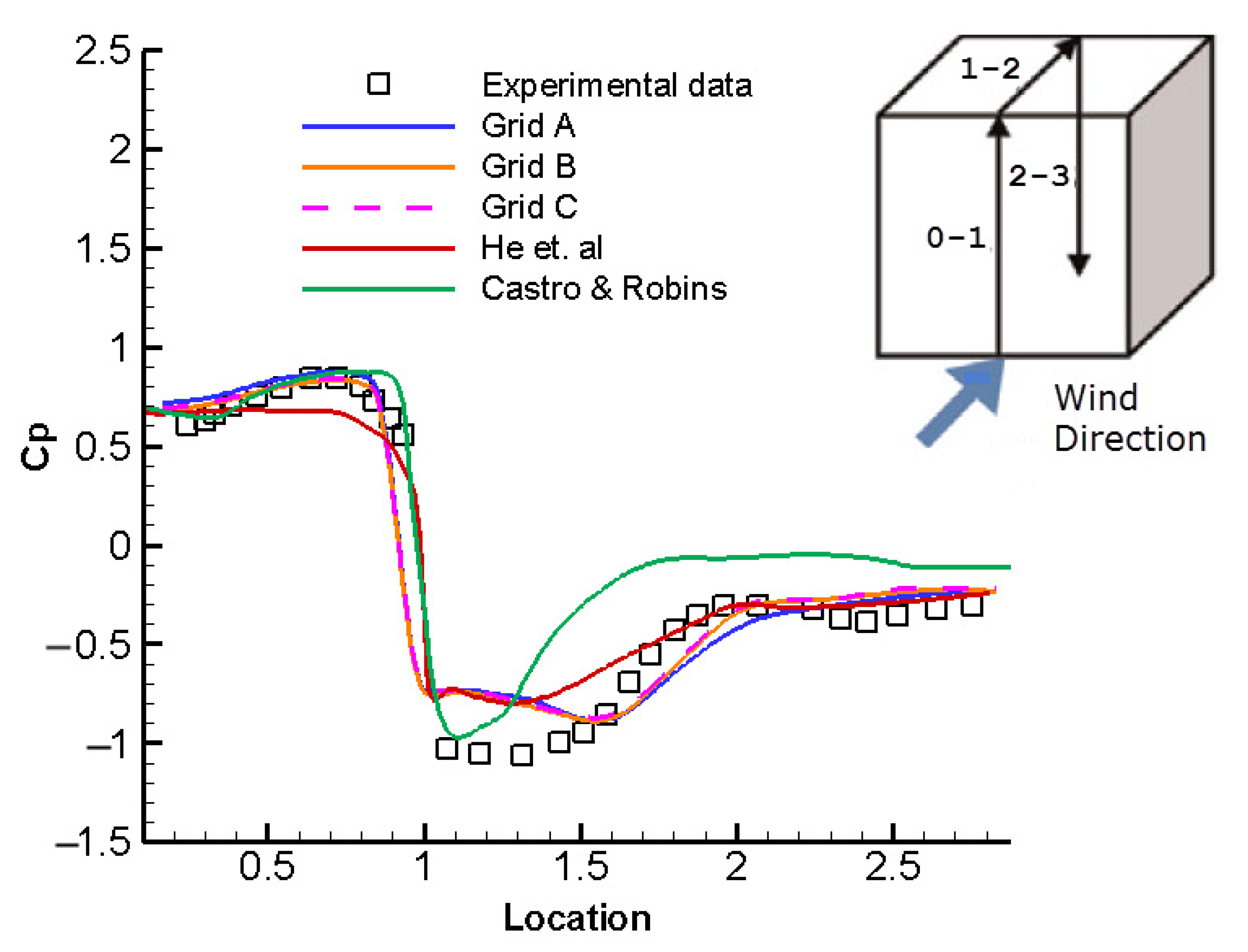
Two sets of experimental data were employed to validate the numerical model of the current study. The first experiment involved measuring the pressure on the vertical and horizontal centrelines of the Silsoe cube of Richards and Hoxey [35]. In this work [35] the full-scale data were sorted out in non-overlapping blocks of cube surface pressure along with the reference upstream flow method measured at the cube height. Because in a full-scale system natural wind conditions are considered, each block of data is exclusive and there is minor or zero chance to accurately repeat a test multiple times, which is not the case in the wind tunnel. As a result, these researchers could process the data in a way that constructs a large number of blocks recorded. The second experiment used the experimental investigation of Castro and Robins [62], who examined the flow around a surface-mounted cube in uniform, irrotational and sheared turbulent flows. The third benchmarking case involved the results of a numerical study on bushfires, wind and structure interactions by He et al. [30], who predicted pressure coefficient distribution around a building under no-fire conditions and compared this with the experimental results measured by others [30].
As mentioned, the Richards and Hoxey experimental data pertaining to the full-scale Silsoe cubic building [31] were used to validate the numerical model in the absence of fire effects. As stated earlier, since the EDC is mostly controlled by turbulent mixing, the fire dynamic characteristics are closely tied with the building aerodynamics. Thus, the pressure distribution over the building in a no-fire scenario is an appropriate indicator showing the accuracy and validity of the numerical results. To minimize numerical uncertainties, a grid sensitivity analysis was conducted. To this end, three sets of different grid sizes were generated. A comparison in terms of numerical settings and computing time on a 24-core node for different grid resolutions is presented in Table 1. All simulations were carried out for a total time of 20 s after fuel injection. It is worth mentioning that a 20 s preliminary run was performed to achieve quasi-fully developed turbulence before the fire source was activated.
The numerical predictions of the mean pressure coefficient along the centrelines over the front, top and rear surfaces of the building (shown by 0–1–2–3 solid lines) are plotted in Figure 2. For a more conclusive comparison, the results of previous numerical studies are also plotted in Figure 2 with those calculated from the three different grids considered in this study. While there is a satisfactory agreement between the experimental and numerical data on both windward and leeward faces (0–1 and 2–3 lines), noticeable discrepancies still exist across the roof face (1–2 line). These discrepancies, which were also present in the other studies included in the figure, can be attributed to the high scatter of wind velocity and direction data, which considerably affects the corner separation region and pressure distribution over the roof. In addition, since the fluctuations of wind pressure on the building are mainly due to large-scale motions [60], the computational domain size could limit the size of the largest eddy and adversely affect the results. While the results for all grid densities give almost the same level of accuracy, it should be noted that smaller scales should also be resolved to simulate turbulent energy exchange in reaction zones accurately [61]. Thus, grid B with a high resolution near the walls was finally selected for further study while grid A was sufficient for aerodynamic performance prediction.
3. Results and Discussion
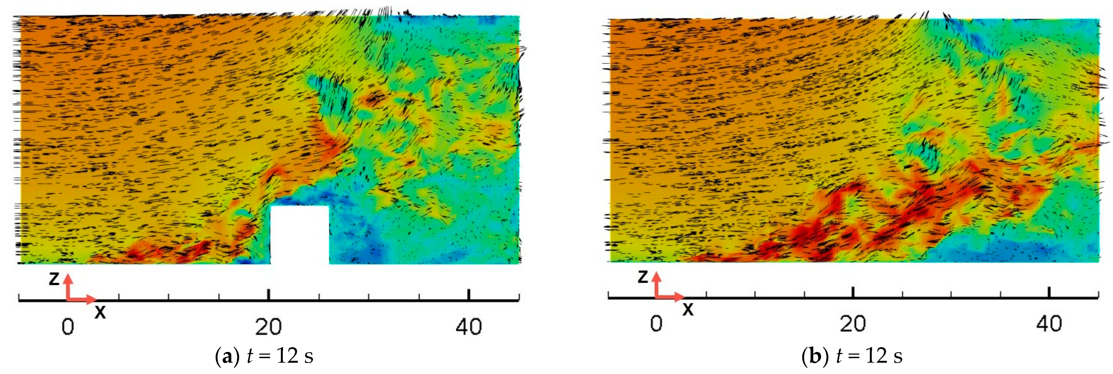
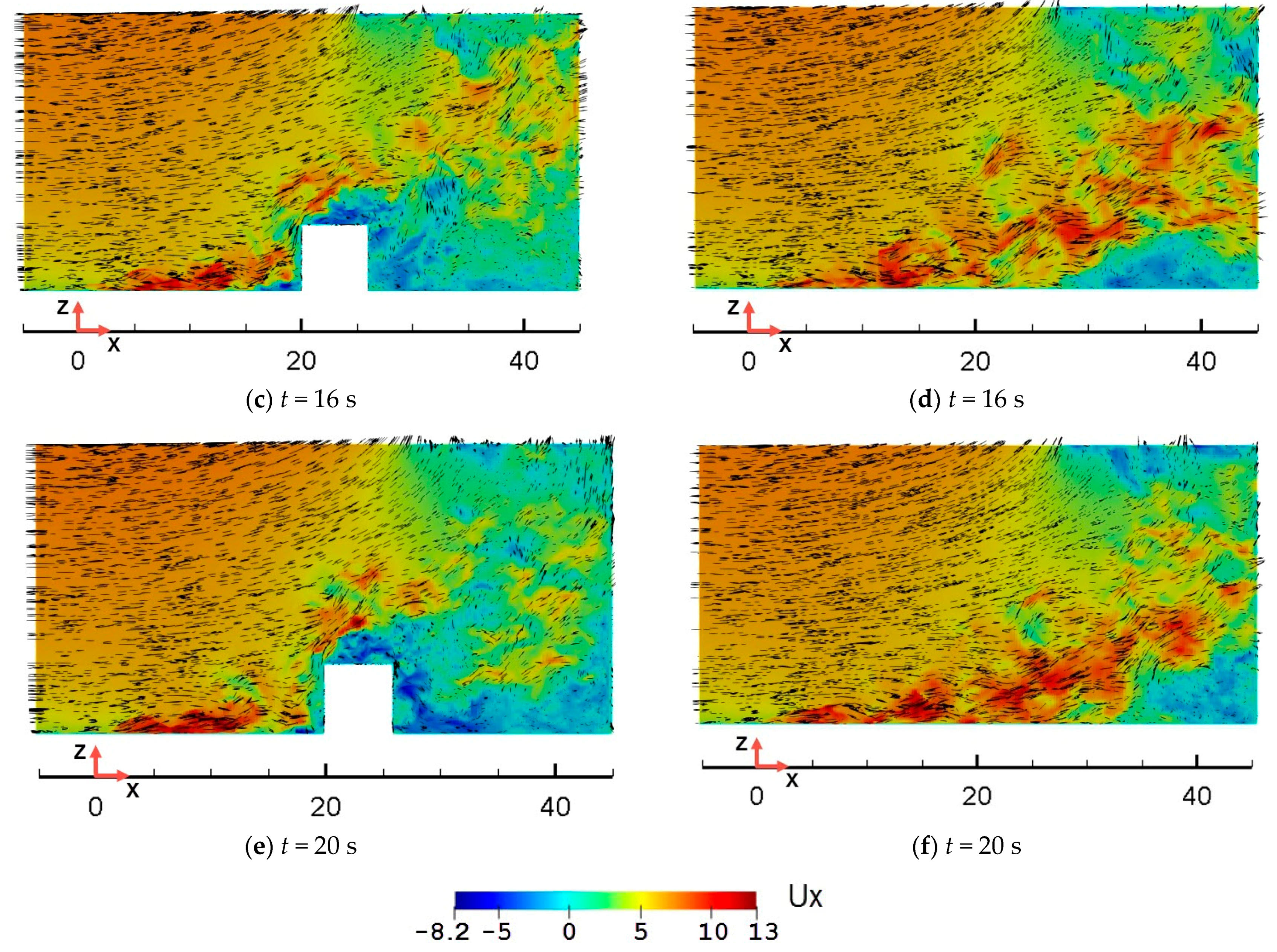
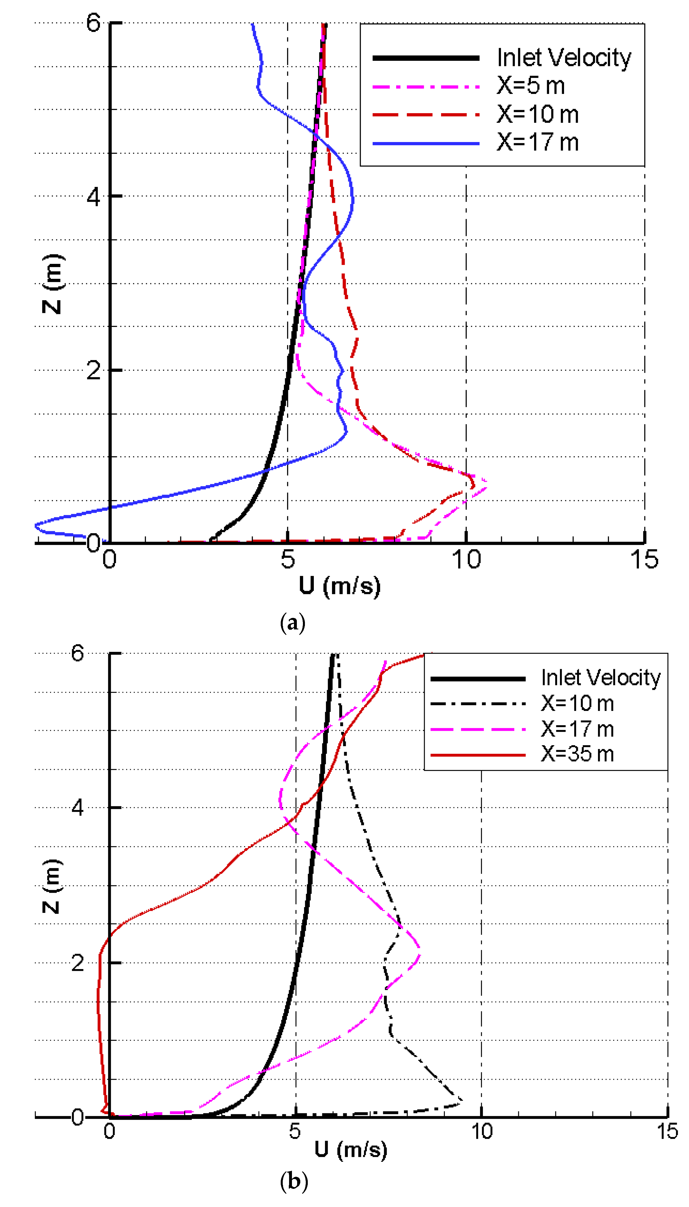
The present study investigated the simulated effect of a dynamically varying wind-field on a stationary heat source, representing a WUI fire configuration. The simulations permitted investigation of the transient fire behaviour that could be expected. Figure 3 shows the time-dependent flow patterns of velocity variation in the fire domain. As shown, the simulated fire front is tilted towards the ground downstream of the fire bed. This is mainly due to the fact that the inertia forces are dominant in this region. In addition, air entrainment into the turbulent surface fire creates a low-pressure region in the flame-ground spacing ahead of the fire. As a result, the fire plume is accelerated and forms a jet-like structure in a relatively small region almost attached to the floor immediately downwind of the fire source. This explanation is consistent with the calculated variation of the velocity profile shown in Figure 4. According to this figure, an intense velocity gradient is observed near the ground (z < 2m) for a specific streamwise length in which a dominant wind-driven fire regime exists. For this fire regime, a large portion of the incoming air passes over the fire plume and is mildly affected by the fire.
Moving further downstream of the fire location, the turbulent boundary flow enters a region where there is no clear balance between buoyant and inertial forcing and as a result, the flame shows random time-dependent motions. The pulsating behaviour of the fire plume propagation leading to the fire intermittency can be reflected in the extent of the attachment region. While the plume attachment region ahead of the building oscillates with a low amplitude, sharp fluctuations (in 27 m < x < 35 m) are observed in the flame-ground contact interface at the adjacent flat areas (see Figure 3b,d,f). Finally, the fire plume encounters a buoyancy-induced reverse flow (coloured in blue in Figure 3) and is driven upward. This phenomenon is often referred to as buoyant instability [63]. As a result, a strong recirculation zone appears, and the low-momentum fire plume eventually separates from the surface. Indeed, the buoyancy-driven fire regime becomes predominant in this region. This effect is further enhanced by the presence of the building blocking part of the incident flow. As shown in Figure 4, beside the building (y = 9 m), where the plume is unimpeded, the plume remains attached to the surface for as far as 35 m downwind from the fire front. In contrast, the plume in the midplane (y = 0 m), where the building acts to block the flow, has already separated from the surface at a distance of only about 17 m downwind from the fire front.
In order to visualize the three-dimensional flow features inside the domain, the Q-criterion [64] is employed. Figure 5 illustrates the vortical structures generated in the presence and absence of fire using Q-Criterion isocontours coloured by the spanwise velocity magnitude in the z-direction to better illustrate buoyancy effects. In the absence of fire, a horse-shoe vortex is formed upstream of the building. This is a common phenomenon as a bluff-body encounters a turbulent boundary layer. Other toroidal and hair-pin vortex cores shedding from the sides of the building are relatively small and are mostly aligned with the streamwise direction. However, as can be seen in Figure 5b, the flow pattern substantially changes in the presence of the fire. In the attachment region, the breakdown of the turbulent boundary layer into small streamwise vortices is highly controlled by the high-momentum flow near the surface. Similar patterns have been reported in experimental observations of laboratory-scale fires, for example [65]. Moving further downstream, as the buoyancy-induced forces become dominant, the flow structures are transformed into larger crosswise vortices creating uplift.
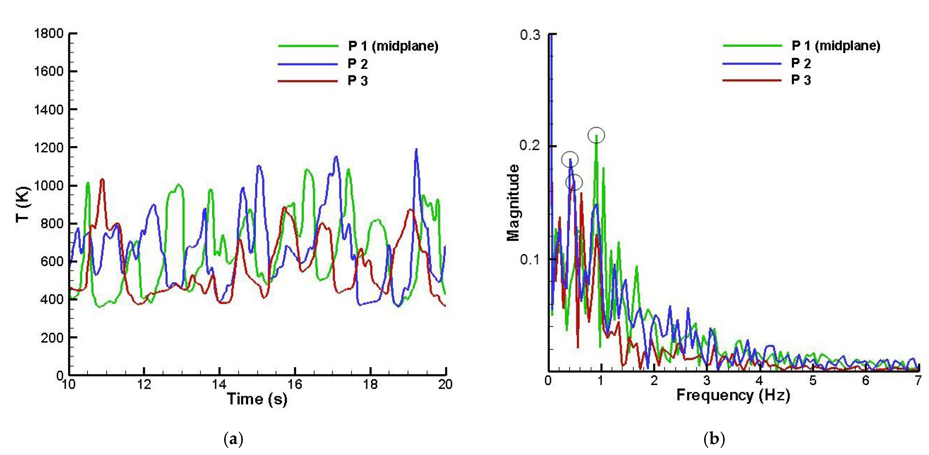
In order to better describe the intermittent behaviour of the unsteady flow in the vicinity of the building, the surface temperature was monitored at three different locations (P1, P2 and P3) in front of the building, as indicated in Figure 1. Figure 6a shows the time-dependent temperature variation obtained at the three monitoring points over a 10 s timeframe (from t = 10 s to 20 s). The temperature fluctuations are mainly caused by the stochastic movement of the flames in the attachment region, which directly affects the fire-surface contact frequency.
The temperature-time series were subject to fast Fourier transform (FFT) analysis, and the dominant frequencies of the temperature signals were calculated. For points P2 and P3, where the fire is spreading over a flat surface (no building), the peak frequencies are nearly the same and occur at f2 = 0.42 Hz and f3 = 0.46 Hz. However, the peak frequency at P1, located in front of the building, is approximately twice (f1 = 0.93 Hz) the frequency at P1 and P2, which suggests that the presence of the building downwind of the fire front results in more frequent pulsations in the fire plume. This can be attributed to premature formation of buoyant instabilities, which manifest in the form of rising crosswise vortices (see Figure 5b) in front of the building. The transient plume behaviour with a higher frequency of pulsation results in more local heating (both radiative and convective heating) around the building, which increases the potential of new ignitions in and around the building; for example, structural extremities (e.g., decking) or sources of fuel that may be present due to lack of household maintenance.
The higher frequency pulsations also mean that the building will be exposed to more frequent convective heating, with less opportunity for convective cooling [65]. This has implications for the likelihood of ignition of finer fuel particles in the vicinity of the structure, including building extremities. It also has implications for the validity of the way flames are represented in risk mitigation frameworks, such as building standards. For example, the Australian Standard for building in bushfire prone areas (AS3959 [66]) bases its calculation of building exposure on a “design fire” concept, in which flames are represented essentially as a static feature rather than the pulsating flames evident in the simulations.
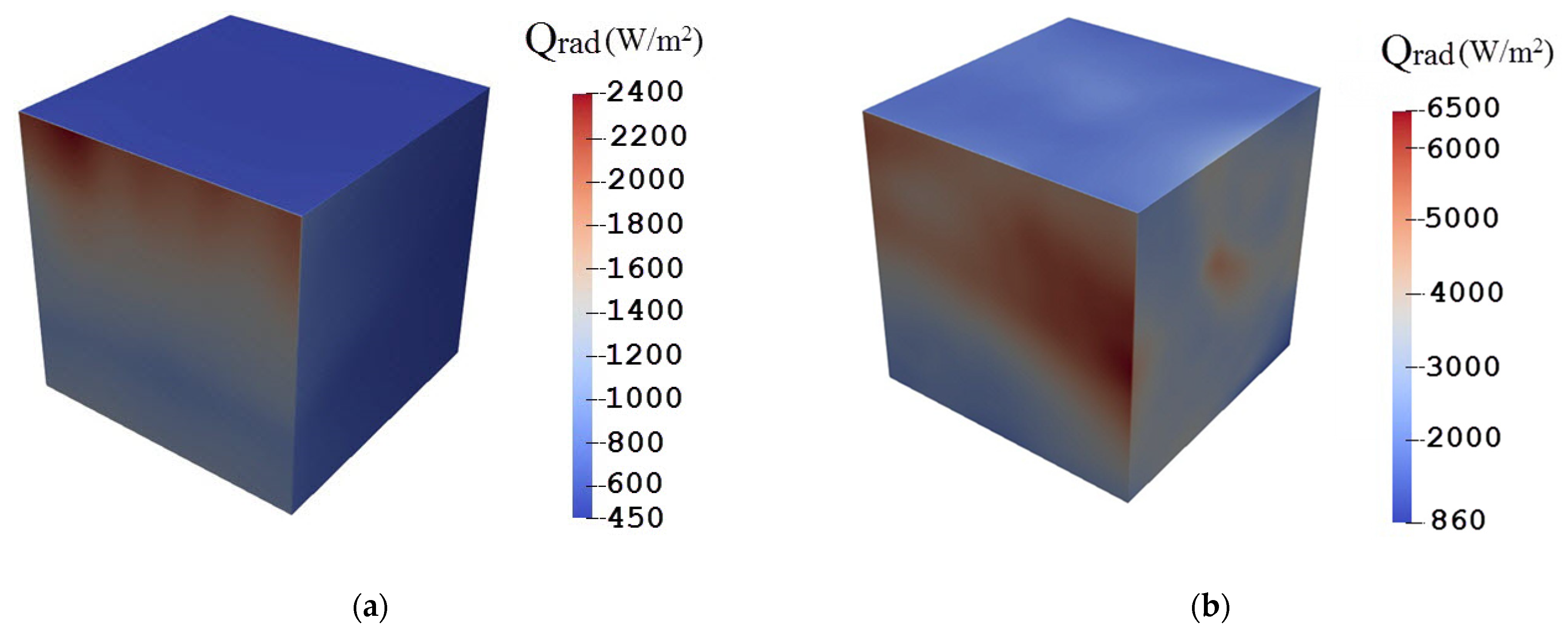
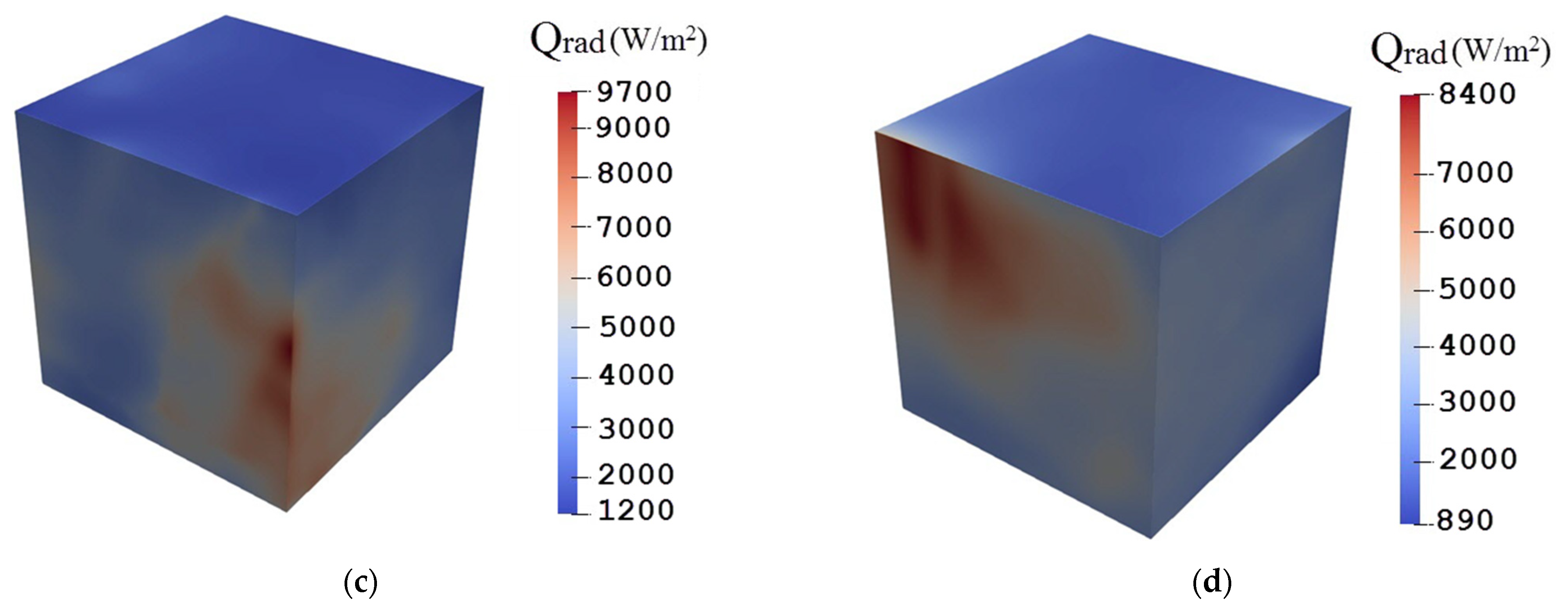
Figure 7 compares the incident radiative heat flux on the building at different times. As expected, the frontal façade of the building receives most of the radiant heat flux over the whole simulation time. At t = 5 s, when the convective plume has not yet fully developed, the heat flux gradually increases with the building height, which is mainly due to the fact that the view factors from the heated ground increase at larger heights. After t = 5 s, a consistent fire plume structure is established, which approximates the effect of a sustained fire front near the building. As a result of the fire’s intermittent pulsing upwind of the building, which occurs after t = 10 s, the pattern of incident radiation becomes highly irregular. The maximum local radiation intensity is observed near the points where the flame extensions and pockets of hot gases come in close contact with the building. On the contrary, the lateral walls and the roof are not exposed to direct fire impingement and therefore experience low exposure to radiation. It is worth mentioning that the local incident heat flux is very close to the critical heat flux for wood pyrolysis [67] (i.e., approximately 10 kW/m2). This suggests that the frontal façade of the building is exposed to a very high risk of thermal pyrolysis compared to the other sides, which are less affected by the fire’s radiant heat.
4. Conclusions
A numerical investigation of the dynamic behaviour of wind-driven surface fires has been presented, with an emphasis on building-fire interaction relevant to consideration of WUI fire impacts. The study was based on LES modelling of a wind-driven fire using the FireFOAM code. The numerical results in the absence of fire were shown to compare well with the data obtained from the full-scale Silsoe building experiments. A comprehensive analysis of the dynamics of the fire’s plume revealed that the building can substantially change the plume attachment length. In other words, the building causes premature buoyant instabilities and the fire plume lift-off distance decreases in front of the building. In addition, an FFT analysis was performed to examine the characteristics of plume pulsations near the building. It was found that the building increases the plume’s intermittency and local heat exchange at some locations upstream of the building. Thus, potentially risky zones susceptible to the generation of new fire sources are formed near the building. In addition, the capability of the present model to predict the thermal response of the building to the fire was studied. These findings provide insights into the likely impacts of wind-driven wildfires applicable to WUI fire scenarios.
Moreover, the results presented here raise some questions about the validity of risk management measures, such as AS3959 [66], in which radiant heat exposure is calculated based on a static “design fire”. In AS3959, flames are essentially considered as a hot surface tilted at a constant angle determined by the balance between wind strength and fire intensity, the latter of which is estimated using quasi-steady fire behaviour models. In contrast, the simulations presented in this study highlight the transient (dynamic) nature of fire propagation and indicate that a fire immediately upwind of a structure can produce flames that alternate between being attached to the surface and more vertically oriented. Flames that are attached to the surface are more likely to bathe a structure in convective heat, and the higher frequency pulsations (between attached/separated regimes) that occur upwind of a structure suggest that convective heating can have a significant influence on the heat exposure of building façades directly in the path of an approaching fire front.
The present study offers a useful framework for evaluating the fire exposure of WUI communities. While it would incur a high computational cost to fully implement the proposed framework at larger scales, this approach could offer a reliable solution to reduce risks from future WUI fires. These findings can be extended by conducting similar studies with fires exhibiting different characteristics (e.g., more or less intense), and realistic building geometries or multiple buildings. In addition, further research is needed to explore fire dynamic behaviour and its impact on smoke dispersion and ember generation in complex urban environments. Such studies are required to inform comprehensive wildfire risk management strategies, including improved urban planning, and WUI building construction design.
Author Contributions
Conceptualization, J.J.S. and M.G. (Maryam Ghodrat); methodology, M.G. (Maryam Ghodrat); software, M.G. (Mohsen Ghaderi); validation, M.G. (Mohsen Ghaderi); formal analysis, M.G. (Mohsen Ghaderi) and M.G. (Maryam Ghodrat); investigation, M.G. (Maryam Ghodrat); resources, M.G. (Maryam Ghodrat); data curation, M.G. (Mohsen Ghaderi) and M.G. (Maryam Ghodrat); writing—original draft preparation, M.G. (Mohsen Ghaderi); writing—review and editing, J.J.S. and M.G. (Maryam Ghodrat); visualization, M.G. (Mohsen Ghaderi); supervision, J.J.S. and M.G. (Maryam Ghodrat); project administration, M.G. (Maryam Ghodrat). All authors have read and agreed to the published version of the manuscript.
Funding
This research received no external funding.
Data Availability Statement
The data presented in this study are available on request from the corresponding author.
Acknowledgments
This research was undertaken with the assistance of resources and services from the National Computational Infrastructure (NCI), which is supported by the Australian Government. The authors are particularly indebted to the NCI for the provision of technical support.
Conflicts of Interest
The authors declare that there are no conflicts of interest regarding the publication of this paper.
Abbreviations
| heat capacity (J/kg/K) | |
| EDC | eddy dissipation concept |
| f | frequency (Hz) |
| g | gravitational acceleration (m/s2) |
| sensible enthalpy (J/kg) | |
| j | mass diffusive flux (kg/m2/s) |
| I | fire intensity (MW/m) |
| number of species | |
| p | pressure (Pa) |
| Pr | Prandtl number |
| heat release per unit volume (W/m3) | |
| radiative flux (W/m2) | |
| Q | heat rate (W) |
| rs | stoichiometric oxygen-to-fuel mass ratio |
| RTE | radiative transfer equation |
| S | strain rate (s-1) |
| Sc | Schmidt number |
| t | time (s) |
| T | temperature (K) |
| U/u | velocity (m/s) |
| Y | mass fraction |
| y+ | dimensionless height of near wall cells |
| Z | height (m) |
| Greek | |
| thermal diffusivity (kg/m/s) | |
| power-law exponent | |
| filter width (m) | |
| heat of combustion (J/kg) | |
| dynamic viscosity (kg/m/s) | |
| kinematic viscosity (m2/s) | |
| density (kg/m3) | |
| mixing time scale (s) | |
| reaction rate (kg/m3/s) | |
| Subscripts | |
| c | combustion |
| F | fuel |
| i, j, k | coordinate index |
| k | species mixture |
| O2 | oxygen |
| r, rad | radiative |
| sgs | sub-grid scale |
| t | turbulent |
| ref | reference value |
| Superscripts | |
| T | transpose |
References
- Walker, X.J.; Baltzer, J.L.; Cumming, S.G.; Day, N.J.; Ebert, C.; Goetz, S.; Johnstone, J.F.; Potter, S.; Rogers, B.M.; Schuur, E.A. Increasing wildfires threaten historic carbon sink of boreal forest soils. Nature 2019, 572, 520–523. [Google Scholar] [CrossRef] [PubMed]
- Theobald, D.M.; Romme, W.H. Expansion of the US wildland–urban interface. Landsc. Urban Plan. 2007, 83, 340–354. [Google Scholar] [CrossRef]
- Mueller, E.V.; Skowronski, N.; Clark, K.; Gallagher, M.R.; Mell, W.E.; Simeoni, A.; Hadden, R.M. Detailed physical modeling of wildland fire dynamics at field scale-An experimentally informed evaluation. Fire Saf. J. 2020, 103051. [Google Scholar] [CrossRef]
- Grishin, A.; Zverev, V.; Shevelev, S.V. Steady-state propagation of top crown forest fires. Combust. Explos. Shock Waves 1986, 22, 733–739. [Google Scholar] [CrossRef]
- Mell, W.; Charney, J.; Jenkins, M.A.; Cheney, P.; Gould, J. Numerical simulations of grassland fire behavior from the LANL-FIRETEC and NIST-WFDS models. In Remote Sensing and Modeling Applications to Wildland Fires; Springer: Berlin/Heidelberg, Germany, 2013; pp. 209–225. [Google Scholar]
- Pimont, F.; Dupuy, J.-L.; Linn, R.R.; Dupont, S. Impacts of tree canopy structure on wind flows and fire propagation simulated with FIRETEC. Ann. For. Sci. 2011, 68, 523. [Google Scholar] [CrossRef] [Green Version]
- Meroney, R.N.; Cairns, N.Q. Numerical prediction of fire propagation in idealized wildland and urban canopies. In Proceedings of the 12th International Conference on Wind Engineering (ICWE12), Cairns, Australia, 1–6 July 2007; pp. 1–6. [Google Scholar]
- Filippi, J.-B.; Bosseur, F.; Pialat, X.; Santoni, P.-A.; Strada, S.; Mari, C. Simulation of coupled fire/atmosphere interaction with the MesoNH-ForeFire models. J. Combust. 2011, 2011, 540390. [Google Scholar] [CrossRef] [Green Version]
- Filippi, J.-B.; Pialat, X.; Clements, C.B. Assessment of ForeFire/Meso-NH for wildland fire/atmosphere coupled simulation of the FireFlux experiment. Proc. Combust. Inst. 2013, 34, 2633–2640. [Google Scholar] [CrossRef]
- Strada, S.; Mari, C.; Filippi, J.-B.; Bosseur, F. Wildfire and the atmosphere: Modelling the chemical and dynamic interactions at the regional scale. Atmos. Environ. 2012, 51, 234–249. [Google Scholar] [CrossRef]
- Rothermel, R.C. A mathematical model for predicting fire spread in wildland fuels. In Intermountain Forest & Range Experiment Station; Forest Service: Washington, DC, USA, 1972; Volume 115. [Google Scholar]
- Finney, M.A.; Andrews, P.L. The Farsite Fire Area Simulator: Fire Management Applications and Lessons of Summer 1994. In Proceedings of the 1994 Interior West Fire Council Meeting and Program, Fairfield, WA, USA, 1–4 November 1994; pp. 209–216. [Google Scholar]
- Balbi, J.-H.; Rossi, J.-L.; Marcelli, T.; Santoni, P.-A. A 3D physical real-time model of surface fires across fuel beds. Combust. Sci. Technol. 2007, 179, 2511–2537. [Google Scholar] [CrossRef]
- Andrews, P.L. BehavePlus Fire Modeling System: Past, Present, and Future. In Proceedings of the 7th Symposium on Fire and Forest Meteorology, Bar Harbor, ME, USA, 23–25 October 2007; American Meteorological Society: Boston, MA, USA, 2017. 13p. [Google Scholar]
- Finney, M.A. FARSITE, Fire Area Simulator—Model Development and Evaluation; US Department of Agriculture, Forest Service, Rocky Mountain Research Station: Fort Collins, CO, USA, 1998.
- Mandel, J.; Beezley, J.D.; Kochanski, A.K. Coupled atmosphere-wildland fire modeling with WRF-fire. arXiv 2011, arXiv:1102.1343. [Google Scholar]
- Kochanski, A.K.; Jenkins, M.A.; Mandel, J.; Beezley, J.D.; Clements, C.B.; Krueger, S. Evaluation of WRF-SFIRE performance with field observations from the FireFlux experiment. Geosci. Model Dev. 2013, 6, 1109–1126. [Google Scholar] [CrossRef] [Green Version]
- Morvan, D.; Accary, G.; Meradji, S.; Frangieh, N.; Bessonov, O. A 3D physical model to study the behavior of vegetation fires at laboratory scale. Fire Saf. J. 2018, 101, 39–52. [Google Scholar] [CrossRef] [Green Version]
- Frangieh, N.; Accary, G.; Morvan, D.; Méradji, S.; Bessonov, O. Wildfires front dynamics: 3D structures and intensity at small and large scales. Combust. Flame 2020, 211, 54–67. [Google Scholar] [CrossRef]
- Eftekharian, E.; Ghodrat, M.; He, Y.; Ong, R.H.; Kwok, K.C.; Zhao, M. Numerical analysis of wind velocity effects on fire-wind enhancement. Int. J. Heat Fluid Flow 2019, 80, 108471. [Google Scholar] [CrossRef]
- Eftekharian, E.; Ghodrat, M.; Ong, R.; He, Y.; Kwok, K. CFD investigation of cross-flow effects on fire-wind enhancement. In Proceedings of the Australasian Fluid Mechanics Conference, Adelaide, Australia, 10–13 December 2018; pp. 10–13. [Google Scholar]
- Eftekharian, E.; Rashidi, M.; Ghodrat, M.; He, Y.; Kwok, K.C. LES simulation of terrain slope effects on wind enhancement by a point source fire. Case Stud. Therm. Eng. 2020, 18, 100588. [Google Scholar] [CrossRef]
- Sullivan, A.L. Wildland surface fire spread modelling, 1990–2007. 1: Physical and quasi-physical models. Int. J. Wildland Fire 2009, 18, 349–368. [Google Scholar] [CrossRef] [Green Version]
- McArthur, A. Fire Behaviour in Eucalypt Forests; Leaflet No. 107; Forest Research Institute, Forestry and Timber Bureau: Canberra, Australia, 1967. [Google Scholar]
- El Houssami, M.; Lamorlette, A.; Morvan, D.; Hadden, R.M.; Simeoni, A. Framework for submodel improvement in wildfire modeling. Combust. Flame 2018, 190, 12–24. [Google Scholar] [CrossRef] [Green Version]
- Linn, R.R.; Goodrick, S.; Brambilla, S.; Brown, M.J.; Middleton, R.S.; O’Brien, J.J.; Hiers, J.K. QUIC-fire: A fast-running simulation tool for prescribed fire planning. Environ. Model. Softw. 2020, 125, 104616. [Google Scholar] [CrossRef]
- Hilton, J.; Leonard, J.; Blanchi, R.; Newnham, G.; Opie, K.; Rucinski, C.; Swedosh, W. Dynamic modelling of radiant heat from wildfires. In Proceedings of the 22nd International Congress on Modelling and Simulation (MODSIM2017), Tasmania, Australia, 3–8 December 2017; pp. 3–8. [Google Scholar]
- Cohen, J.D. Relating flame radiation to home ignition using modeling and experimental crown fires. Can. J. For. Res. 2004, 34, 1616–1626. [Google Scholar] [CrossRef]
- Mell, W.E.; Manzello, S.L.; Maranghides, A.; Butry, D.; Rehm, R.G. The wildland–urban interface fire problem–current approaches and research needs. Int. J. Wildland Fire 2010, 19, 238–251. [Google Scholar] [CrossRef]
- He, Y.; Kwok, K.; Douglas, G.; Razali, I. Numerical investigation of bushfire-wind interaction and its impact on building structure. Fire Saf. Sci. 2011, 10, 1449–1462. [Google Scholar] [CrossRef]
- Richards, P.; Hoxey, R. Pressures on a cubic building—Part 1: Full-scale results. J. Wind Eng. Ind. Aerodyn. 2012, 102, 72–86. [Google Scholar] [CrossRef]
- Fryanova, K.; Perminov, V. Impact of Forest Fires on Buildings and Structures. Available online: https://elib.spbstu.ru/dl/2/j18-445.pdf/info (accessed on 1 November 2020).
- Pimont, F.; Dupuy, J.-L.; Linn, R. Fire effects on the physical environment in the WUI using FIRETEC. Phys. Based Fire Model Eval. Valid. 2014. [Google Scholar] [CrossRef] [Green Version]
- Almeida, Y.P.; Lage, P.L.; Silva, L.F.L. Large eddy simulation of a turbulent diffusion flame including thermal radiation heat transfer. Appl. Therm. Eng. 2015, 81, 412–425. [Google Scholar] [CrossRef]
- Sikanen, T.; Hostikka, S. Modeling and simulation of liquid pool fires with in-depth radiation absorption and heat transfer. Fire Saf. J. 2016, 80, 95–109. [Google Scholar] [CrossRef]
- Manzello, S.L.; Suzuki, S.; Gollner, M.J.; Fernandez-Pello, A.C. Role of firebrand combustion in large outdoor fire spread. Prog. Energy Combust. Sci. 2020, 76, 100801. [Google Scholar] [CrossRef]
- Hakes, R.S.; Salehizadeh, H.; Weston-Dawkes, M.J.; Gollner, M.J. Thermal characterization of firebrand piles. Fire Saf. J. 2019, 104, 34–42. [Google Scholar] [CrossRef] [Green Version]
- Tohidi, A.; Kaye, N.B. Stochastic modeling of firebrand shower scenarios. Fire Saf. J. 2017, 91, 91–102. [Google Scholar] [CrossRef]
- Jasak, H.; Jemcov, A.; Tukovic, Z. OpenFOAM: A C++ library for complex physics simulations. In Proceedings of the International Workshop on Coupled Methods in Numerical Dynamics, Dubrovnik, Croatia, 19–21 September 2007; pp. 1–20. [Google Scholar]
- Richards, P.; Norris, S. LES modelling of unsteady flow around the Silsoe cube. J. Wind Eng. Ind. Aerodyn. 2015, 144, 70–78. [Google Scholar] [CrossRef]
- Byram, G.M. Combustion of forest fuels. In Forest Fire: Control and Use; McGraw-Hill: New York, NY, USA, 1959; pp. 61–89. [Google Scholar]
- Lund, T.S.; Wu, X.; Squires, K.D. Generation of turbulent inflow data for spatially-developing boundary layer simulations. J. Comput. Phys. 1998, 140, 233–258. [Google Scholar] [CrossRef] [Green Version]
- Wu, X. Inflow turbulence generation methods. Annu. Rev. Fluid Mech. 2017, 49, 23–49. [Google Scholar] [CrossRef]
- Bonnet, J.-P.; Delville, J.; Lamballais, E. The Generation of Realistic 3D, Unsteady Inlet Conditions for LES. In Proceedings of the 41st Aerospace Sciences Meeting and Exhibit, Reno, NV, USA, 6–9 January 2003; p. 65. [Google Scholar]
- Davidson, L. Hybrid LES-RANS: Inlet boundary conditions for flows including recirculation. In Proceedings of the Fifth International Symposium on Turbulence and Shear Flow Phenomena, Munich, Germany, 27–29 August 2007. [Google Scholar]
- Tominaga, Y.; Mochida, A.; Yoshie, R.; Kataoka, H.; Nozu, T.; Yoshikawa, M.; Shirasawa, T. AIJ guidelines for practical applications of CFD to pedestrian wind environment around buildings. J. Wind Eng. Ind. Aerodyn. 2008, 96, 1749–1761. [Google Scholar] [CrossRef]
- Launder, B.E.; Spalding, D.B. The numerical computation of turbulent flows. In Numerical Prediction of Flow, Heat Transfer, Turbulence and Combustion; Elsevier: Amsterdam, The Netherlands, 1983; pp. 96–116. [Google Scholar]
- Versteeg, H.K.; Malalasekera, W. An Introduction to Computational Fluid Dynamics: The Finite Volume Method; Pearson Education: London, UK, 2007. [Google Scholar]
- Maragkos, G.; Rauwoens, P.; Wang, Y.; Merci, B. Large eddy simulations of the flow in the near-field region of a turbulent buoyant helium plume. Flow Turbul. Combust. 2013, 90, 511–543. [Google Scholar] [CrossRef]
- Wang, Y.; Chatterjee, P.; de Ris, J.L. Large eddy simulation of fire plumes. Proc. Combust. Inst. 2011, 33, 2473–2480. [Google Scholar] [CrossRef]
- Liu, H.; Wang, C.; Zhang, A. Numerical simulation of the wood pyrolysis with homogenous/heterogeneous moisture using FireFOAM. Energy 2020, 201, 117624. [Google Scholar] [CrossRef]
- Myers, T.; Trouvé, A.; Marshall, A. Predicting sprinkler spray dispersion in FireFOAM. Fire Saf. J. 2018, 100, 93–102. [Google Scholar] [CrossRef]
- Ren, N.; Wang, Y.; Vilfayeau, S.; Trouvé, A. Large eddy simulation of turbulent vertical wall fires supplied with gaseous fuel through porous burners. Combust. Flame 2016, 169, 194–208. [Google Scholar] [CrossRef]
- Poinsot, T.; Veynante, D. Theoretical and Numerical Combustion; RT Edwards, Inc.: Montgomery, PA, USA, 2005. [Google Scholar]
- Favre, A. Turbulence: Space-time statistical properties and behavior in supersonic flows. Phys. Fluids 1983, 26, 2851–2863. [Google Scholar] [CrossRef]
- Spotz, R.B.E. The Kinetic Theory of Gases30 J. 0. Hirschfelder CF Curtiss. In High Speed Aerodynamics and Jet Propulsion: Thermodynamics and Physics of Matter; Rossini, F.D., Ed.; Princeton University Press: Princeton, NJ, USA, 1955; Volume 1. [Google Scholar]
- Mills, A. Heat Transfer USA; CRC Press: Boca Raton, FL, USA, 1992. [Google Scholar]
- Nicoud, F.; Ducros, F. Subgrid-scale stress modelling based on the square of the velocity gradient tensor. FlowTurbul. Combust. 1999, 62, 183–200. [Google Scholar] [CrossRef]
- Magnussen, B.F.; Hjertager, B.H. On mathematical modeling of turbulent combustion with special emphasis on soot formation and combustion. Symp. Combust. 1977, 16, 719–729. [Google Scholar] [CrossRef]
- Coppalle, A.; Vervisch, P. The total emissivities of high-temperature flames. Combust. Flame 1983, 49, 101–108. [Google Scholar] [CrossRef]
- Jasak, H. Error Analysis and Estimation for the Finite Volume Method with Applications to Fluid Flows. Ph.D. Thesis, University of London, London, UK, 1996. [Google Scholar]
- Castro, I.; Robins, A. The flow around a surface-mounted cube in uniform and turbulent streams. J. Fluid Mech. 1977, 79, 307–335. [Google Scholar] [CrossRef]
- Verma, M.K. Physics of Buoyant Flows: From Instabilities to Turbulence; World Scientific: Singapore, 2018. [Google Scholar]
- Dubief, Y.; Delcayre, F. On coherent-vortex identification in turbulence. J. Turbul. 2000, 1, 11. [Google Scholar] [CrossRef]
- Finney, M.A.; Cohen, J.D.; Forthofer, J.M.; McAllister, S.S.; Gollner, M.J.; Gorham, D.J.; Saito, K.; Akafuah, N.K.; Adam, B.A.; English, J.D. Role of buoyant flame dynamics in wildfire spread. Proc. Natl. Acad. Sci. USA 2015, 112, 9833–9838. [Google Scholar] [CrossRef] [Green Version]
- Debnam, G.; Chow, V.; England, P. AS 3959 Construction of Buildings in Bushfire-Prone Areas–Draft for Public Comment (Dr 05060) Review of Calculation Methods and Assumptions; Warrington Fire Research: Melbourne, Australia, 2005. [Google Scholar]
- Tran, H.C.; Cohen, J.D.; Chase, R.A. Modeling Ignition of Structures in Wildland/Urban Interface Fires; Inter Science Communications: Gosport, UK, 1992. [Google Scholar]
Figure 1.
Schematic of the computational domain and the location of the refinement zone (shaded with grey colour) and temperature monitoring points.
Figure 1.
Schematic of the computational domain and the location of the refinement zone (shaded with grey colour) and temperature monitoring points.

Figure 2.
Comparison of the measured mean pressure coefficients calculated for three different grid resolutions with experimental data [31] and numerical results reported by He et al. [30] and Castro & Robins [62]; The measurements were taken on the building centreline shown by the solid line of (0–1–2–3); Uref = 6 m/s (no-fire case).

Figure 3.
Vertical transects of instantaneous streamwise velocity component () and corresponding velocity vectors ( = 6 m/s, = 12 s, 16 s, 20 s) at different lateral locations. (a) = 12 s, = 0 m (b) = 12 s, = 9 m (c) = 16 s, = 0 m (d) = 16 s, = 9 m (e) = 20 s, = 0 m (f) = 20 s, = 9 m
Figure 3.
Vertical transects of instantaneous streamwise velocity component () and corresponding velocity vectors ( = 6 m/s, = 12 s, 16 s, 20 s) at different lateral locations. (a) = 12 s, = 0 m (b) = 12 s, = 9 m (c) = 16 s, = 0 m (d) = 16 s, = 9 m (e) = 20 s, = 0 m (f) = 20 s, = 9 m


Figure 4.
Vertical profiles of longitudinal velocity at different longitudinal positions (Uref = 6 m/s, t = 20 s) aligned with the (a) midplane Y = 0 (b) section plane at Y = 9 m.
Figure 4.
Vertical profiles of longitudinal velocity at different longitudinal positions (Uref = 6 m/s, t = 20 s) aligned with the (a) midplane Y = 0 (b) section plane at Y = 9 m.

Figure 5.
Instantaneous isosurfaces of the Q-criterion (t = 20 s) coloured by velocity component. (a) In the absence of fire, and (b) in the presence of fire.
Figure 5.
Instantaneous isosurfaces of the Q-criterion (t = 20 s) coloured by velocity component. (a) In the absence of fire, and (b) in the presence of fire.

Figure 6.
(a) Time history of instantaneous surface temperature; (b) frequency spectrum of temperature obtained from fast Fourier transform (FFT) analysis; dominant frequencies are marked with circles.
Figure 6.
(a) Time history of instantaneous surface temperature; (b) frequency spectrum of temperature obtained from fast Fourier transform (FFT) analysis; dominant frequencies are marked with circles.

Figure 7.
Instantaneous radiative heat flux at different times: (a) t = 5 s, (b) t = 10 s, (c) t = 15 s, (d) t = 20s.
Figure 7.
Instantaneous radiative heat flux at different times: (a) t = 5 s, (b) t = 10 s, (c) t = 15 s, (d) t = 20s.


Table 1.
Computational grid specifications and numerical settings.
| ID | Number of Cells (Millions) | y+ | Timestep (s) | Computing Time (Hours) |
|---|---|---|---|---|
| grid A | 4.6 | 37 | 0.004 | 16 |
| grid B | 7.8 | 1.65 | 0.0015 | 62 |
| grid C | 9.5 | 0.95 | 0.0015 | 71 |
Publisher’s Note: MDPI stays neutral with regard to jurisdictional claims in published maps and institutional affiliations. |
© 2020 by the authors. Licensee MDPI, Basel, Switzerland. This article is an open access article distributed under the terms and conditions of the Creative Commons Attribution (CC BY) license (http://creativecommons.org/licenses/by/4.0/).
Share and Cite
MDPI and ACS Style
Ghaderi, M.; Ghodrat, M.; Sharples, J.J. LES Simulation of Wind-Driven Wildfire Interaction with Idealized Structures in the Wildland-Urban Interface. Atmosphere 2021, 12, 21. https://0-doi-org.brum.beds.ac.uk/10.3390/atmos12010021
AMA Style
Ghaderi M, Ghodrat M, Sharples JJ. LES Simulation of Wind-Driven Wildfire Interaction with Idealized Structures in the Wildland-Urban Interface. Atmosphere. 2021; 12(1):21. https://0-doi-org.brum.beds.ac.uk/10.3390/atmos12010021
Chicago/Turabian StyleGhaderi, Mohsen, Maryam Ghodrat, and Jason J. Sharples. 2021. "LES Simulation of Wind-Driven Wildfire Interaction with Idealized Structures in the Wildland-Urban Interface" Atmosphere 12, no. 1: 21. https://0-doi-org.brum.beds.ac.uk/10.3390/atmos12010021
Note that from the first issue of 2016, this journal uses article numbers instead of page numbers. See further details here.