Complex Networks Reveal Teleconnections between the Global SST and Rainfall in Southwest China


1
Data Science Research Center, Faculty of Science, Kunming University of Science and Technology, Kunming 650500, China
2
Department of Physics, Bar-Ilan University, Ramat Gan 52900, Israel
3
Laboratory for Climate Studies, National Climate Research Center CMA, Beijing 100081, China
4
College of Physics and Electronic Engineering, Changshu Institute of Technology, Suzhou 215100, China
*
Authors to whom correspondence should be addressed.
Atmosphere 2021, 12(1), 101; https://0-doi-org.brum.beds.ac.uk/10.3390/atmos12010101
Submission received: 9 December 2020
/
Revised: 31 December 2020
/
Accepted: 8 January 2021
/
Published: 12 January 2021
(This article belongs to the Special Issue New Approaches to Complex Climate Systems)
Abstract
:Droughts and floods have frequently occurred in Southwest China (SWC) during the past several decades. Yet, the understanding of the mechanism of precipitation in SWC is still a challenge, since the East Asian monsoon and Indian monsoon potentially influence the rainfall in this region. Thus, the prediction of precipitation in SWC has become a difficult and critical topic in climatology. We develop a novel multi-variable network-based method to delineate the relations between the global sea surface temperature anomalies (SSTA) and the precipitation anomalies (PA) in SWC. Our results show that the out-degree patterns in the Pacific, Atlantic and Indian Ocean significantly influence the PA in SWC. In particular, we find that such patterns dominated by extreme precipitation change with the seasons. Furthermore, we uncover that the teleconnections between the global SSTA and rainfall can be described by the in-degree patterns, which dominated by several vital nodes within SWC. Based on the characteristics of these nodes, we find that the key SSTA areas affect the pattern of the nodes in SWC with some specific time delays that could be helpful to improve the long-term prediction of precipitation in SWC.
1. Introduction
During the recent decades, natural hazards (such as droughts and floods) have occurred frequently in Southwest China (SWC) due to climate change, causing numerous casualties and property losses [1,2]. In the summer of 2006 and 2011, SWC suffered from record-breaking droughts events [3]. On the other hand, the portion of annual precipitation contributed by extremely heavy precipitation has been found as a result of an increasing trend in the period of 1961–2010 [4]. Due to the population growth and high risk of natural hazards, SWC has attracted lots of attention in the meteorological research fields. According to the CMIP5 multi-model projections, severe and extreme droughts in SWC will increase dramatically in the future, meanwhile, extremely wet events will also increase [5].
Droughts and floods can be attributed to precipitation anomalies. A better understanding of precipitation can further improve the underlying mechanisms of droughts and floods in SWC. It was reported that the annual precipitation over SWC does not show a significant decreasing or increasing trend [3,6]. In fact, the trend of precipitation in SWC has been found to strongly depend on spatiotemporal patterns [4,7]. The forecasting of precipitation in SWC is very challenging, since it can be influenced by both the East Asian monsoon and Indian monsoon which could carry moist air from both the Indian Ocean and the Pacific Ocean to SWC [8,9,10,11]. Previous studies have found that some correlations between the SSTA and precipitation in SWC based on the regression analysis and the Empirical Orthogonal Functions (EOFs) [12,13]. Nevertheless, such traditional analyses cannot describe well the connection contained in the daily time series and present the nonlinear behaviors of complex systems, i.e., time delay in systems [14].
Complex networks approach has been successfully applied to a wide variety of complex systems in the past decade [15,16,17]. It also emerged as a powerful tool to study climate systems [18,19,20,21]. Here, the geographic sites or grids are considered as the network nodes, and the linear or nonlinear interactions between any pair of nodes are regarded as the network edges or links [18,21]. The strength of the link is quantified by the cross-correlation. Complex networks can analyze the dynamics of the climate system systematically [22,23,24,25,26], and some applications of complex networks in climate science have improved the understanding of some climate phenomenon [27,28,29,30]. The El Niño phenomenon can be predicted one year ahead in advance by using the network method [31,32], the prediction skill is even better than some dynamical models. Some features of air pollution have also been detected by the network approach [33]. Recently, the network method provided a great insight into the function of the Rossby waves in creating stable, global-scale dependency of extreme-rainfall events, and revealed the teleconnection features of extreme rainfall events [34]. Furthermore, extreme precipitation events can be predicted even in a long-term scale in some cases by using the networks [35].
Indeed, the network-based method has shown many merits in extreme rainfall analysis and prediction. Yet, (i) the correlations between the global SSTA and extreme rainfall in SWC have not been studied by the network approach; (ii) whether the teleconnections and the precursor signals exist to potentially improve the prediction of rainfall in SWC? In order to overcome the two problems, we develop a multi-variable network approach here to analyze the relationship between the global SSTA and the precipitation anomalies (PA) in SWC for different seasons. The structure of our paper is as follows: In the second part we will introduce the data and method; the main results are shown in the third part; finally, we give a short summary.
2. Data and Methodology
2.1. Data
The data is obtained from the global ERA-interim reanalysis of the European Centre for Medium-Range Weather Forecasts (https://www.ecmwf.int/) [36]. We use the daily averaged precipitation in SWC with a resolution of and the global SST with a resolution of from January 1979 to December 2017. The spatial range of SWC is and , resulting grid points. We choose this area is since that it mainly represents the SWC and its surrounding areas. We totally have grid points for the global SST. Due to the seasonality of rainfall, we divide the entire time series of precipitation in SWC into four seasons, i.e., Spring (March-April-May, MAM), Summer (June-July-August, JJA), Autumn (September-October-November, SON) and Winter (December-January-February, DJF), respectively.
2.2. Methodology
Firstly, we remove the seasonal cycle to obtain the time series of the SSTA as [37,38],
where is the time series of the daily SST. stands the year and stands date within a year. The “” and “” denote the mean and standard deviation of the SST. We perform the same analysis to obtain the precipitation anomalies (PA).
We then construct the directed and weighted multi-variable network. Network nodes and can be classified into two subsets by two different variables, one subset denotes the PA nodes over SWC and the other denotes the global SSTA nodes. We divide one year into four seasons, e.g., JJA for summer as mentioned in Data. For the days in summers, we can obtain their dates for 39 years and respectively define the daily time series of grid i for the PA and grid j for the SSTA as, and , where spans the dates and is the time delay (the dates of shift days in relative to the dates of . The negative means that the SSTA is ahead the precipitation, vice versa. The cross-correlation function is written as [37,39],
where is the time lag, days. 〈 〉 is averaged for all . We identify the largest absolute value of and denote the corresponding time lag as . The correlation between the site and is defined as . We define that the direction of the link is from to when and from to when . The direction is undefined when .
To obtain the adjacency matrix of the network, a threshold is introduced to exclude noise and only the links from the SSTA to PA are considered [39]. Thus the adjacency matrix is defined as:
If , there is a link between and . If , there is no link between them. Then the proportion of the positive links is calculated by,
where is the latitude for the SSTA node and is introduced as a weight for the link regarding the area size i.e., the pole is just a point and its area size is zero and the area size for a gird in the Equator is biggest [14]. Similarly, we obtain the proportion of the negative links .
The extent of the SSTA nodes to influence the PA nodes in the network is usually quantified by the weighted out-degree [37,39]. We define the weighted out-degree of the node as:
The positive and negative degrees can more information about positive and negative correlations respectively than the totally degree. We have that is divided into the positive and negative weighted out-degrees and by the weight , respectively.
To find the important nodes in SWC which are strongly influenced by the most SSTA areas, the weighted in-degree of the PA node is defined as:
Also we obtain the positive and negative weighted in-degrees and .
3. Results
3.1. Significance Tests
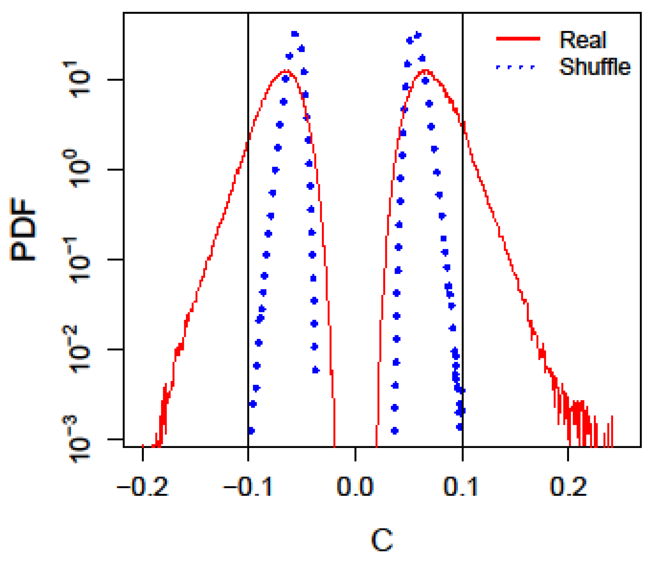
According to Equation (2), we obtain for any pair of nodes between the global SSTA and PA in SWC for four different seasons respectively. Figure 1 shows the probability distribution function (PDF) of their corresponding correlation . We find two separated peaks related to positive, and negative correlations, respectively in Figure 1. It further demonstrates the differences between positive and negative correlations. In order to verify the significance of the correlation, we compare the PDFs between the real data and shuffled data as shown Figure 1. Here, we randomly shuffle the order of years for each node, keeping the variations within each year to get shuffle data [37]. Then, we calculate the cross-correlation for the shuffled data. In such shuffling process, the autocorrelations and common seasonality have been kept, while the physical dependencies between the SSTA and PA nodes are destroyed. The PDF of the real data in Figure 1 shows a much slower decay than the shuffle data for both the positive and negative parts. Therefore, it proves that some correlations are non-random. If the correlations are significantly higher than the significant threshold ∆, we regard them as real links; otherwise, they are suspected to be spurious links as Equation (3). We obtain the threshold ∆ = 0.1 by using the 99.5% confidence significance test.
3.2. Links and Degrees
We obtain the proportions of positive and negative links and by Equation (4) and calculate the averages of correlations for positive and negative links as , in Table 1. In Table 1, we summarize the statistics of the positive and negative links for four seasons. We find the largest proportion for positive links in MAM and the largest for negative links in DJF (see Table 1). Both the strongest correlations and are also found in MAM. The fewest positive and negative links are observed in SON. The correlations and also are weakest for SON. Therefore, the connections between the SSTA and PA in SWC strongly depend on seasons.
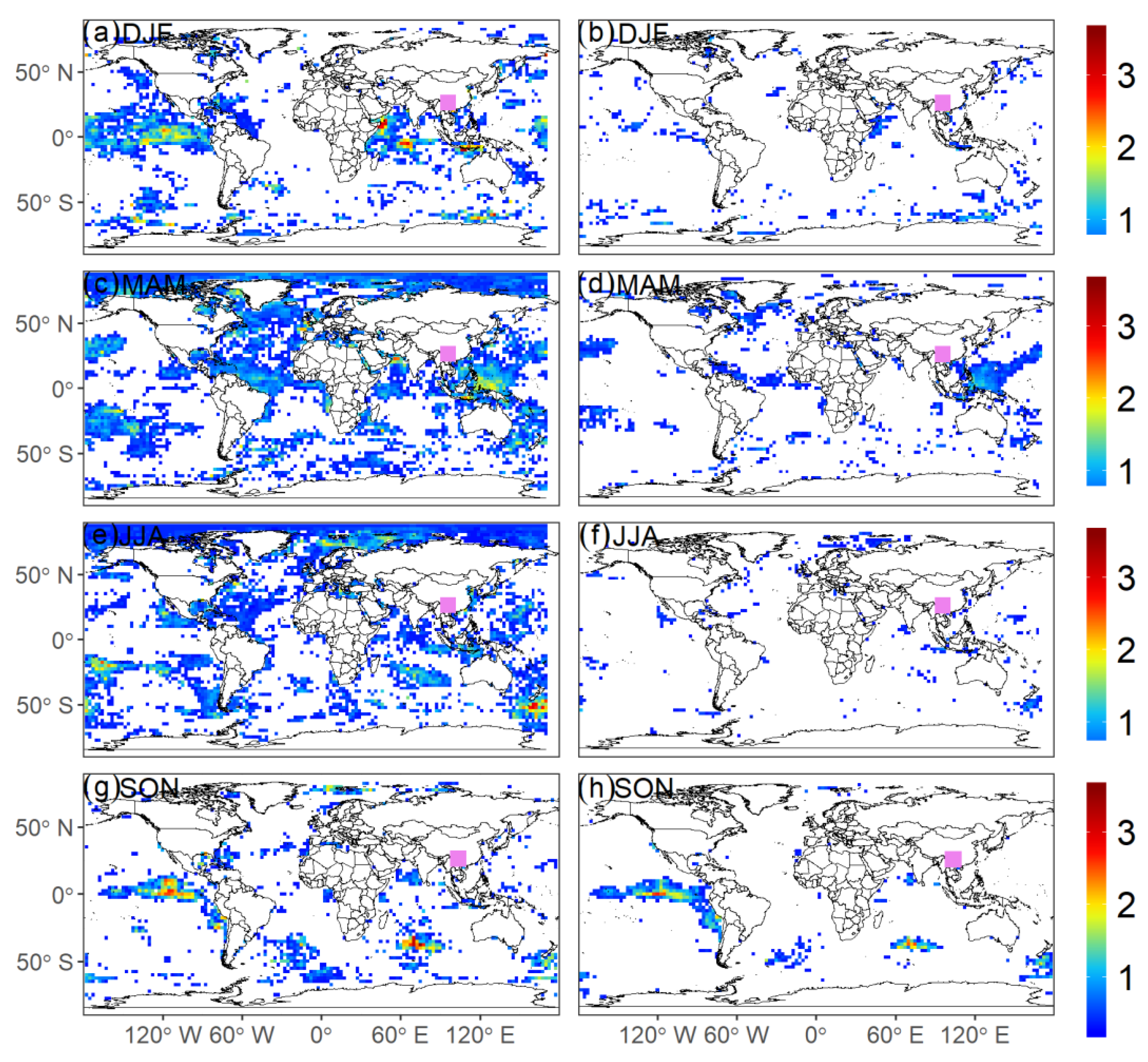
Then we present the global out-degree pattern according to Equation (5). The out-degree patterns show that some important regions on the oceans are significant correlated with the PA of SWC in different seasons. In DJF, the nodes that have strong positive out-degree are located in the north Indian Ocean and east Equatorial Pacific in Figure 2a. In contrast, the locations of these nodes move to the Equatorial Atlantic Ocean and west Equatorial Pacific in MAM. Note that the nodes in the east Equatorial Pacific disappeared in Figure 2c. For JJA, Figure 2e shows that the nodes with high degrees can be found in high latitudes but not around the Equator. In SON, a few strong nodes are found locating in the east Equatorial Pacific and the south Indian Ocean. Due to the special geographical location of SWC, both the East Asian monsoon and Indian monsoon carry moist air from the Indian Ocean and Pacific Ocean to SWC resulting in extreme precipitation. Therefore, we suggest that these important out-degree areas and SWC are connected through the bridge function of the East Asian monsoon and Indian monsoon [40,41,42,43]. Different features of the monsoons can be used to explain the changes of the degree patterns in different seasons.
To further test the contribution of extreme precipitation to the degree patterns, top and bottom 5% extreme PA data are replaced by the random middle magnitude PA. Then we perform the same analysis to the new time series. Figure 2b,d,f,h show the results. Comparing with Figure 2a for real data, much less significant nodes are observed in the Oceans in Figure 2b. Still, few nodes are in the same locations. Similar results can also be found for other seasons. It implies that extreme precipitation plays an important role in forming the teleconnection degree patterns.
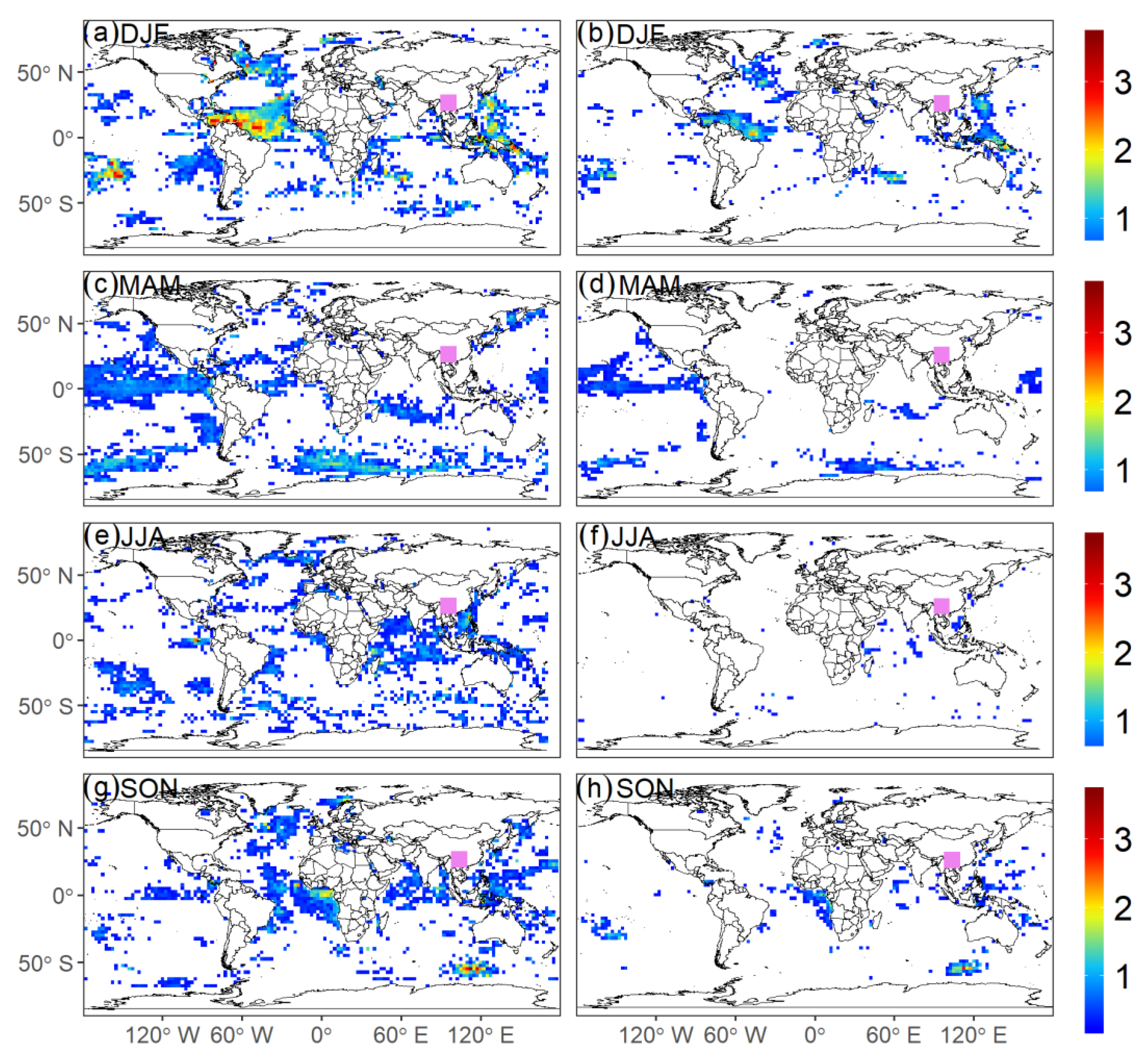
The distributions of the negatively weighted out-degree are shown in Figure 3. We find that they are very different form the positive case. For instance, we find some major negative degree patterns in the Equatorial Atlantic and west Equatorial Pacific, and few nodes in the east Equatorial Pacific for DJF (see Figure 3a), which are the opposite of the results for the positive weighted out-degree in Figure 2a. Similar results are also found for other seasons (see Figure 3c,e,g). In fact, there are correlations for the SSTA itself between the two regions i.e., the SSTA in the east Equatorial Pacific is negative correlated with the SSTA in the west Equatorial Pacific. Such anti-correlations can lead to the positive and negatively correlated patterns between the PA in SWC and SSTA in the two different regions.
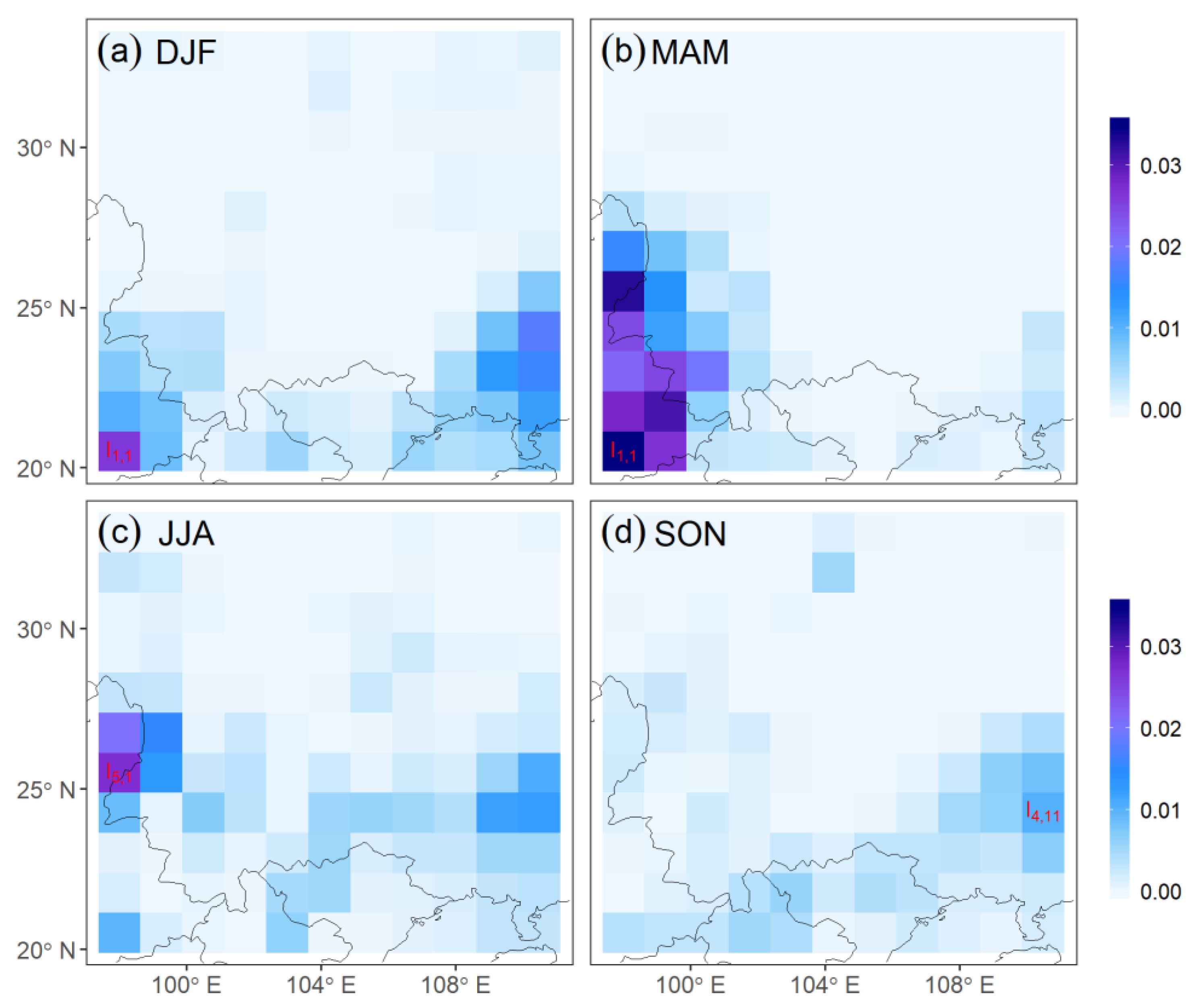
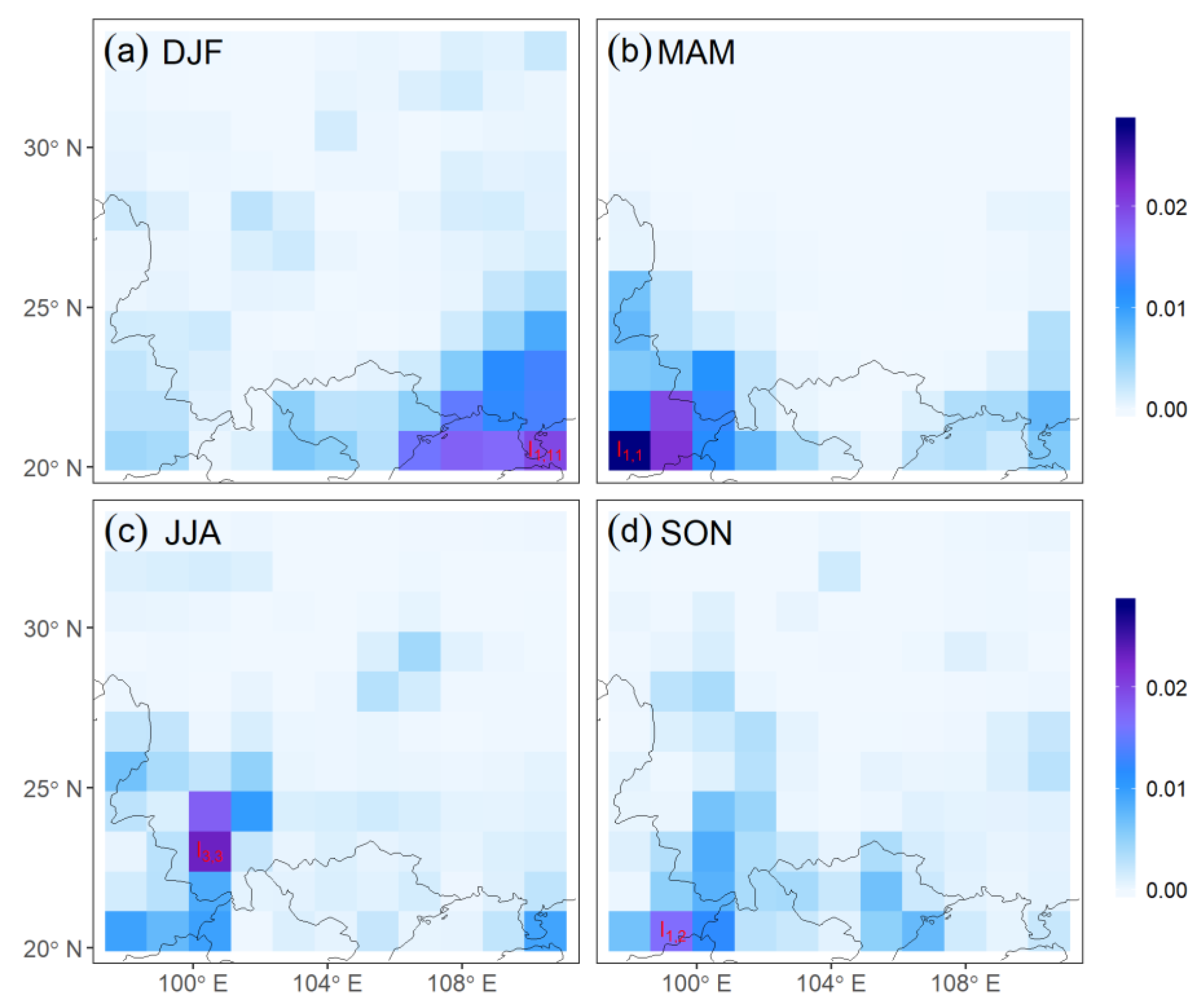
The PA in different locations within SWC could be influenced by different weather systems as suggested by Ma et al. [4] and Shi et al. [7]. To test the correlations between the SSTA and PA nodes, we calculate the weighted in-degree for the PA nodes by Equation (6). We find that some nodes within SWC have small in-degree values and several nodes have strong correlations with the SSTA as shown in Figure 4 and Figure 5. The spatial distribution of in-degree is inhomogeneous and varies with seasons. The important nodes with large in-degree values are almost located in the left- and right- bottom corners of SWC which are close to the Indian, and west Pacific Ocean, respectively. Therefore, these nodes of SWC are easier to be influenced by the Indian and the East Asian monsoons than other nodes in SWC. Note that the largest positive and negative weighted in-degree nodes are the same for MAM (see Figure 4b and Figure 5b). It implies that the most sensitive region in SWC respect to the SSTA can keep both two kinds of correlations.
3.3. Important Areas
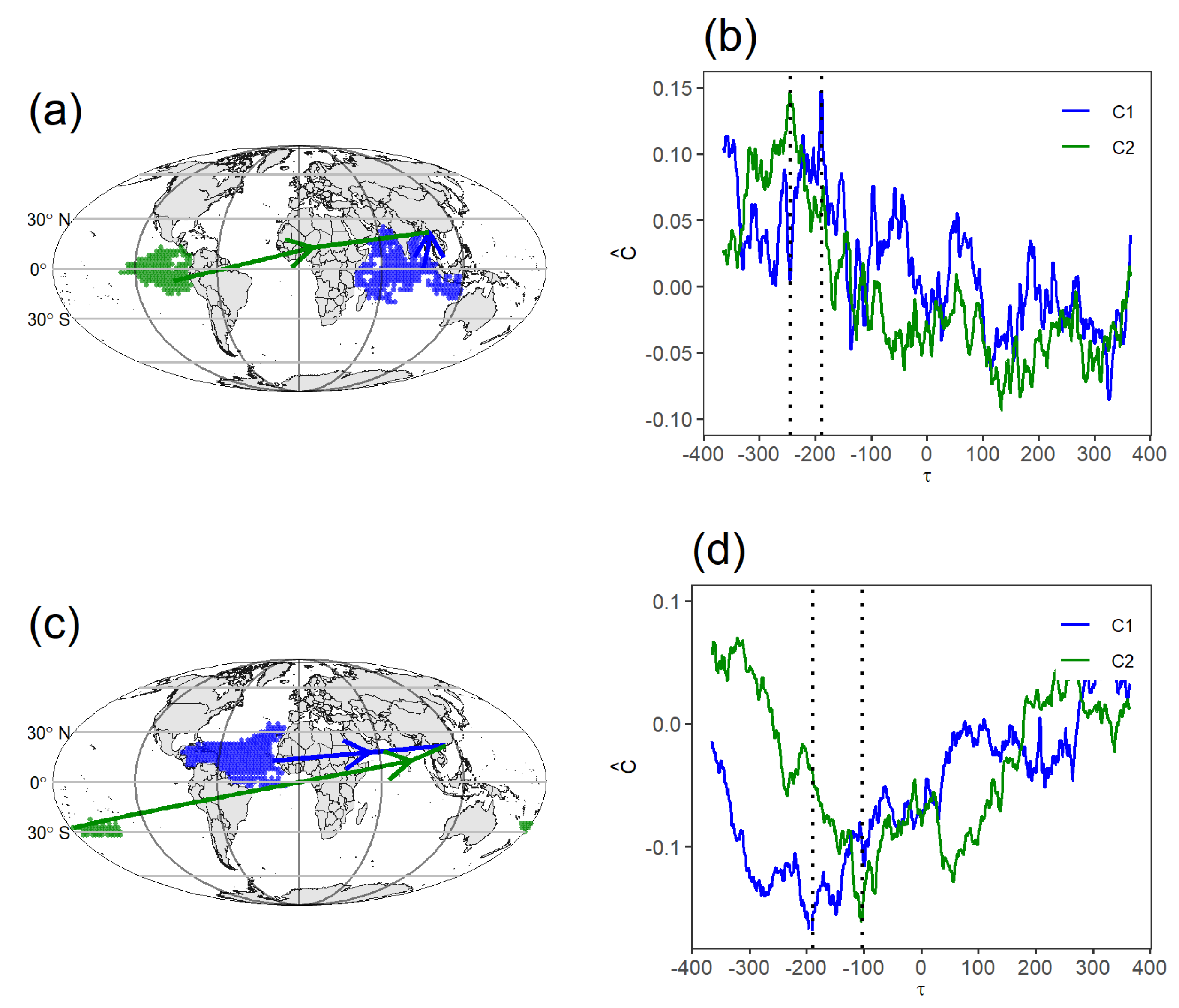
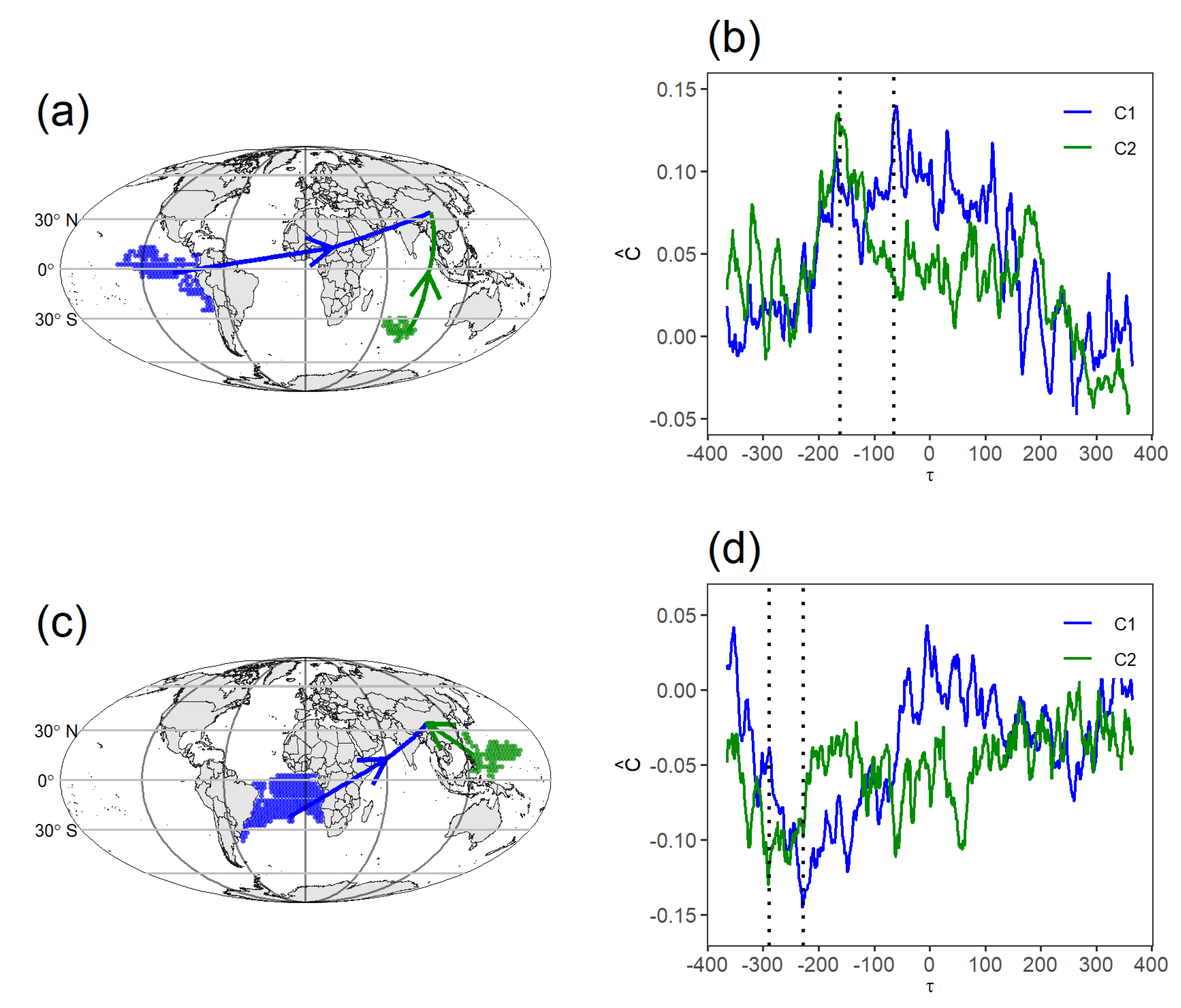
Since the inhomogeneous influence on SWC’s PA is observed, we next consider the connection between the important nodes within SWC and the largest clusters of the SSTA. We first select the nodes in SWC with the largest weighted in-degrees (which are more than 4 times standard deviation above the averaged degree) for each season as shown in Figure 4 and Figure 5. The largest cluster is identified by the largest successive area where all the inside SSTA nodes are connected to that important node in SWC. We can obtain the second largest cluster by using a similar way. Figure 6a shows the cluster (blue) and (green) are connected to the nodes (as shown in Figure 4a) for DJF. Both of them are positively correlated to in DJF. We show the strongest links for and in Figure 6a and their time delays in Figure 6b. The correlation changes with the time lag and reaches to the maximum value at −189 days for and −245 days for in Figure 6b. Similar time delays are also observed for the other links between and different SSTA nodes within the clusters. Therefore, the cluster in the east Equatorial Pacific performs a longer time delay that could be useful for long-term prediction. The reason could be related to the El Niño—Southern Oscillation that arouses warm SST in the central and east Equatorial Pacific at the beginning, then lead to temperature anomaly in the Indian Ocean [42,44]. The PA in SWC can be significantly influenced by the El Niño through the bridge of the East Asian monsoon and Indian monsoon [44]. We show that the cluster and are negatively correlated with the nodes (as shown in Figure 5a) for DJF in Figure 6c. The cluster locates in the Equatorial Atlantic that can arouse a series of quasi-stationary wave trains. Such waves can propagate eastward leading to an anticyclone (cyclone) in upper air of SWC, and motivating (inhibiting) PA [42]. The time delay corresponding to the maximum correlation is −190 days for the strongest link of (see Figure 6d). There is a similar time delay −104 days for the link of in the Middle East Pacific (see Figure 6d).
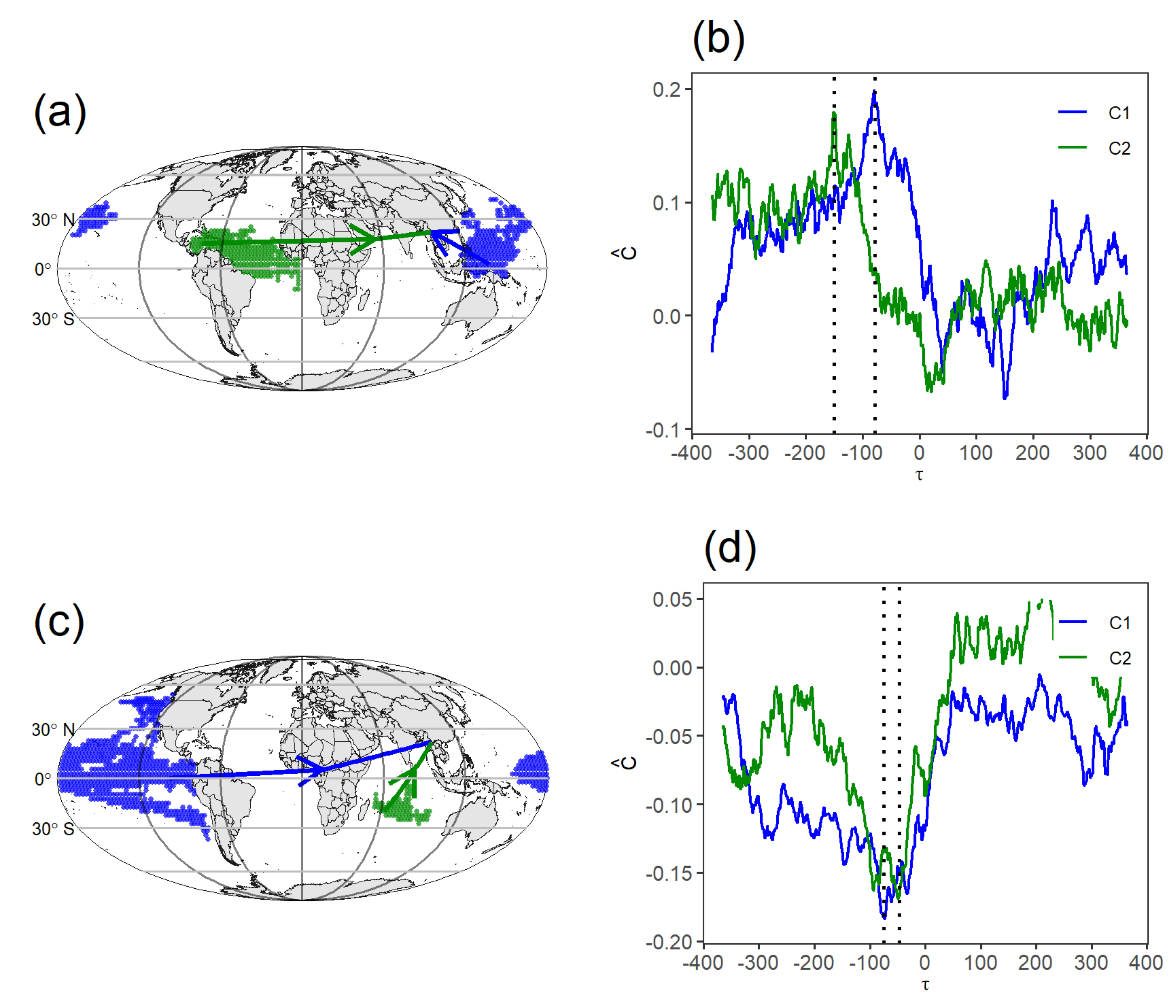
For MAM, the links between the SSTA and PA in SWC are much higher than other three seasons. The largest cluster size is also larger than other seasons. Figure 7a shows that the cluster in the west Pacific and in the Equatorial Atlantic are positively correlated with the nodes in MAM. For the negative correlation, however, the clusters and mainly distributed in the east Pacific and Indian Ocean (see Figure 7c). Therefore, most of the correlation patterns come from the Pacific, which implies that the SSTA in the tropical Pacific has a crucial impact on PA in SWC. Moreover, the time delays of the strongest links for are within 100 days shorter than that of DJF, but the strength of links is stronger (Figure 7b,d). Therefore, we suggest that the proceeding winter SSTA probably influences the PA in MAM. The SSTA in the east Pacific often reaches to the peak during winter [40]. It will further influence the circulation systems, i.e., the Walker atmospheric circulation and the Hadley circulation in the tropical Pacific then cause climate anomalies in East Asia including SWC after around three months.
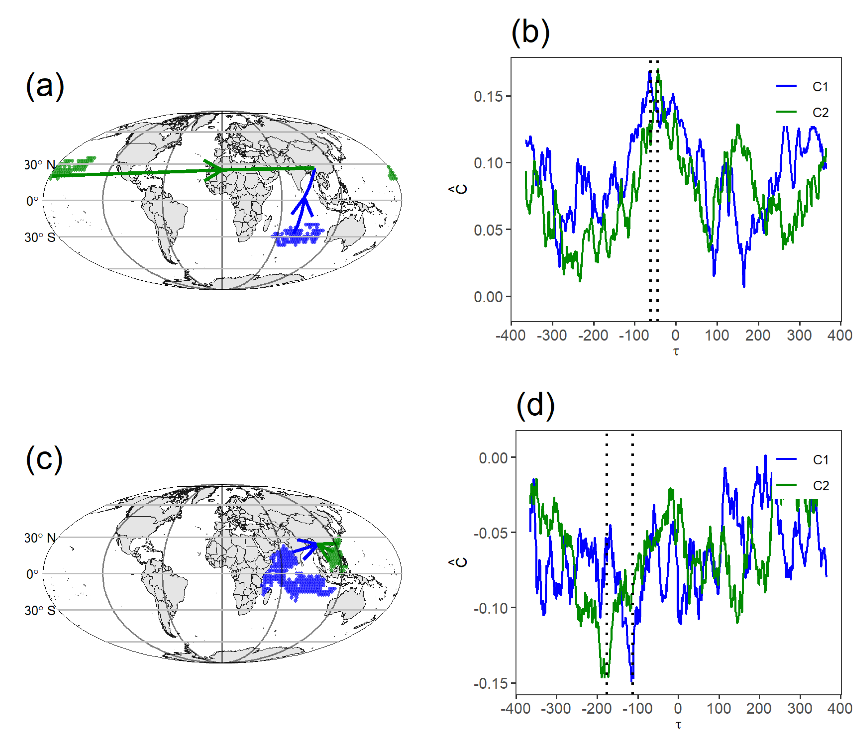
Figure 8 and Figure 9 show the same analysis as Figure 6 and Figure 7, but for JJA and SON, respectively. We find that the cluster sizes are smaller and the correlations are weaker than DJF and MAM. This is given that much more moisture is generated by local sources in SWC for JJA. Besides, we also find that the Indian Ocean and Pacific are important areas to influence the SWC in JJA and SON. Thus, considering both the Indian Ocean and Pacific could better improve the prediction of the rainfall in SWC [45,46].
4. Conclusions
In this study, we employ a multi-variable complex network method to study the teleconnection between the SSTA and PA in SWC. We reveal that there are the most links between PA in SWC and the global SSTA network in Spring, followed by Winter, Summer and Autumn, respectively. According to the weighted out-degree of the network, we show the positive and negative correlation patterns over the global and find that most of the out-degree patterns emerge in the Equatorial Indian, Pacific and Atlantic Oceans which are mainly contributed by extreme PA in SWC. The mechanisms could be related to atmospheric bridge function of East Asian and Indian monsoons for the Equatorial Indian and Pacific Oceans. For the links between SWC and the Atlantic SSTA, the long-range Atlantic, long-range planetary waves account for the teleconnections [42,47]. The seasonal variation of the East Asian and Indian monsoon system mainly presents south wind in Summer and north wind in Winter, which can result that the out-degree patterns change with seasons.
According to the weighted in-degree in SWC, we find that the teleconnections are dominated by some important nodes. Therefore, we obtain the two largest clusters in the Oceans which are connected to the important nodes in the SWC. The time delay of the strongest link between the tropical east Pacific cluster and the important node of SWC is respectively −245 days for DJF, −75 days for MAM, −62 days for JJA, and −65 days for SON. Such teleconnection patterns over the global and their time delays for four seasons have not been reported in previous studies. These results are based on a complex network analysis and could be useful in improving the prediction of rainfall in SWC. The potential rainfall prediction and its mechanism need further analysis based on climate models and observation data.
Author Contributions
W.L., Z.G. and Y.Z. designed research; P.Q. performed research; P.Q. and Y.Z. analyzed data; P.Q., W.L., Y.Z. and Z.G. wrote the paper. P.Q., W.L., Y.Z. and Z.G. contributed to reviewing the manuscript. All authors have read and agreed to the published version of the manuscript.
Funding
This research was supported by the National Key Research and Development Program of China (2018YFC1507702) and the National Natural Science Foundation of China Project (Grant Nos. 61573173, 42075057 and 41875100).
Institutional Review Board Statement
Not applicable.
Informed Consent Statement
Not applicable.
Data Availability Statement
The data in this paper was downloaded from the European Centre for Medium-Range Weather Forecasts (https://www.ecmwf.int/).
Acknowledgments
We are grateful for the data resources provided by the European Centre for Medium-Range Weather Forecasts. And thanks to Fan Jingfang for helping to revise the paper.
Conflicts of Interest
The authors declare no conflict of interest. The funders had no role in the design of the study; in the collection, analyses, or interpretation of data; in the writing of the manuscript; or in the decision to publish the results.
References
- Gao, J.; Sang, Y. Identification and estimation of landslide-debris flow disaster risk in primary and middle school campuses in a mountainous area of Southwest China. Int. J. Disaster Risk Reduct. 2017, 25, 60–71. [Google Scholar] [CrossRef]
- Wei, L.; Hu, K.; Hu, X. Rainfall occurrence and its relation to flood damage in China from 2000 to 2015. J. Mt. Sci. 2018, 15, 2492–2504. [Google Scholar] [CrossRef]
- Zhang, C.; Tang, Q.; Chen, D.; Li, L.; Liu, X.; Cui, H. Tracing changes in atmospheric moisture supply to the drying Southwest China. Atmos. Chem. Phys. Discuss. 2017, 17, 10383–10393. [Google Scholar] [CrossRef] [Green Version]
- Ma, Z.; Liu, J.; Zhang, S.-Q.; Chen, W.-X.; Yang, S.-Q. Observed Climate Changes in Southwest China during 1961–2010. Adv. Clim. Chang. Res. 2013, 4, 30–40. [Google Scholar] [CrossRef]
- Wang, L.; Chen, W.; Zhou, W. Assessment of future drought in Southwest China based on CMIP5 multimodel projections. Adv. Atmos. Sci. 2014, 31, 1035–1050. [Google Scholar] [CrossRef]
- Qin, N.; Chen, X.; Fu, G.; Zhai, J.; Xue, X. Precipitation and temperature trends for the Southwest China: 1960–2007. Hydrol. Process. 2010, 24, 3733–3744. [Google Scholar] [CrossRef]
- Shi, P.; Wu, M.; Qu, S.; Jiang, P.; Qiao, X.; Chen, X.; Zhou, M.; Zhang, Z. Spatial Distribution and Temporal Trends in Precipitation Concentration Indices for the Southwest China. Water Resour. Manag. 2015, 29, 3941–3955. [Google Scholar] [CrossRef]
- Zhang, R. Relations of Water Vapor Transport from Indian Monsoon with That over East Asia and the Summer Rainfall in China. Adv. Atmos. Sci. 2001, 18, 1005–1017. [Google Scholar] [CrossRef]
- Qian, W.; Kang, H.-S.; Lee, D.K. Distribution of seasonal rainfall in the East Asian monsoon region. Theor. Appl. Clim. 2002, 73, 151–168. [Google Scholar] [CrossRef]
- Wang, L.; Chen, W.; Zhou, W.; Huang, G. Teleconnected influence of tropical Northwest Pacific sea surface temperature on interannual variability of autumn precipitation in Southwest China. Clim. Dyn. 2015, 45, 2527–2539. [Google Scholar] [CrossRef]
- Wang, L.; Huang, G.; Chen, W.; Zhou, W.; Wang, W. Wet-to-dry shift over Southwest China in 1994 tied to the warming of tropical warm pool. Clim. Dyn. 2018, 51, 3111–3123. [Google Scholar] [CrossRef]
- Xia, Y.; Guan, Z.Y.; Long, Y. Relationships between convective activity in the Maritime Continent and precipitation anomalies in Southwest China during boreal summer. Clim. Dyn. 2020, 54, 973–986. [Google Scholar] [CrossRef]
- Jiang, X.; Shu, J.; Wang, X.; Hu, X.; Wu, Q. The Roles of Convection over the Western Maritime Continent and the Philippine Sea in Interannual Variability of Summer Rainfall over Southwest China. J. Hydrometeo. 2017, 18, 2043–2056. [Google Scholar] [CrossRef]
- Steinhaeuser, K.; Chawla, N.V.; Ganguly, A.R. Complex networks as a unified framework for descriptive analysis and predictive modeling in climate science. Stat. Anal. Data Min. 2011, 4, 497–511. [Google Scholar] [CrossRef]
- Barabã¡si, A.-L.; Albert, R. Emergence of Scaling in Random Networks. Science 1999, 286, 509–512. [Google Scholar] [CrossRef] [PubMed] [Green Version]
- Barrat, A.; Barthelemy, M.; Pastor-Satorras, R.; Vespignani, A. The architecture of complex weighted networks. Proc. Natl. Acad. Sci. USA 2004, 101, 3747–3752. [Google Scholar] [CrossRef] [Green Version]
- Zhang, Y.W.; Hu, G.K.; Chen, X.S.; Chen, W.; Liu, W.Q. Study of the shear-rate dependence of granular friction based on community detection. Sci. China-Phys. Mech. Astron. 2019, 62, 40511. [Google Scholar] [CrossRef]
- Donges, J.F.; Zou, Y.; Marwan, N.; Kurths, J. Complex networks in climate dynamics. Eur. Phys. J. Spéc. Top. 2009, 174, 157–179. [Google Scholar] [CrossRef] [Green Version]
- Liess, S.; Kumar, A.; Snyder, P.K.; Kawale, J.; Steinhaeuser, K.; Semazzi, F.H.M.; Ganguly, A.R.; Samatova, N.F.; Kumar, V. Different Modes of Variability over the Tasman Sea: Implications for Regional Climate*. J. Clim. 2014, 27, 8466–8486. [Google Scholar] [CrossRef] [Green Version]
- Zhou, D.; Gozolchiani, A.; Ashkenazy, Y.; Havlin, S. Teleconnection Paths via Climate Network Direct Link Detection. Phys. Rev. Lett. 2015, 115, 268501. [Google Scholar] [CrossRef] [Green Version]
- Fan, J.F.; Meng, J.; Ludescher, J.; Chen, X.S.; Ashkenazy, Y.; Kurths, J.; Havlin, S.; Schellnhuber, H.J. Statistical physics approaches to the complex Earth system. Phys. Rep. 2020. [Google Scholar] [CrossRef] [PubMed]
- Boers, N.; Bookhagen, B.; Marwan, N.; Kurths, J.; Marengo, J.A. Complex networks identify spatial patterns of extreme rainfall events of the South American Monsoon System. Geophys. Res. Lett. 2013, 40, 4386–4392. [Google Scholar] [CrossRef] [Green Version]
- Tsonnis, A.A.; Swanson, K.L. Topology and Predictability of El Niño and La Niña Networks. Phys. Rev. Lett. 2008, 100, 228502. [Google Scholar] [CrossRef] [Green Version]
- Yamasaki, K.; Gozolchiani, A.; Havlin, S. Climate Networks around the Globe are Significantly Affected by El Niño. Phys. Rev. Lett. 2008, 100, 228501. [Google Scholar] [CrossRef] [PubMed]
- Guez, O.; Gozolchiani, A.; Berezin, Y.; Wang, Y.; Havlin, S. Global climate network evolves with North Atlantic Oscillation phases: Coupling to Southern Pacific Ocean. EPL Europhys. Lett. 2013, 103, 68006. [Google Scholar] [CrossRef] [Green Version]
- Lu, Z.H.; Yuan, N.M.; Fu, Z.T. Percolation Phase Transition of Surface Air Temperature Networks under Attacks of Attacks of El Niño/La Niña. Sci. Rep. 2016, 6, 26779. [Google Scholar] [CrossRef] [PubMed] [Green Version]
- Gong, Z.Q.; Zhou, L.; Zhi, R.; Feng, G.L. Analysis of Dynamical Statistical Characteristics of Temperature Correlation Networks of 1-30D Scales. Acta Phys. Sin. 2008, 57, 5351–5360. [Google Scholar] [CrossRef]
- Barreiro, M.; Marti, A.C.; Masoller, C. Inferring long memory processes in the climate network via ordinal pattern analysis. Chaos Interdiscip. J. Nonlinear Sci. 2011, 21, 013101. [Google Scholar] [CrossRef] [Green Version]
- Steinhaeuser, K.; Ganguly, A.R.; Chawla, N.V. Multivariate and multiscale dependence in the global climate system revealed through complex networks. Clim. Dyn. 2012, 39, 889–895. [Google Scholar] [CrossRef]
- Zhang, Y.W.; Fan, J.F.; Li, X.T.; Liu, W.Q.; Chen, X.S. Evolution mechanism of principal modes in climate dynamics. New J. Phys. 2020, 22, 093077. [Google Scholar] [CrossRef]
- Ludescher, J.; Gozolchiani, A.; Bogachev, M.I.; Bunde, A.; Havlin, S.; Schellnhuber, H.J. Very early warning of next El Niño. Proc. Natl. Acad. Sci. USA 2014, 111, 2064–2066. [Google Scholar] [CrossRef] [PubMed] [Green Version]
- Meng, J.; Fan, J.F.; Ludescher, J.; Agarwal, A.; Chen, X.S.; Bunde, A.; Kurths, J.; Schellnhuber, H.J. Complexity based approach for El Niño magnitude forecasting before the “spring predictability barrier”. Proc. Natl. Acad. Sci. USA 2020, 117, 177–183. [Google Scholar] [CrossRef] [PubMed] [Green Version]
- Zhang, Y.; Fan, J.; Chen, X.; Ashkenazy, Y.; Havlin, S. Significant Impact of Rossby Waves on Air Pollution Detected by Network Analysis. Geophys. Res. Lett. 2019, 46, 12476–12485. [Google Scholar] [CrossRef] [Green Version]
- Boers, N.; Goswami, B.; Rheinwalt, A.; Bookhagen, B.; Hoskins, B.; Kurths, J. Complex networks reveal global pattern of extreme-rainfall teleconnections. Nat. Cell Biol. 2019, 566, 373–377. [Google Scholar] [CrossRef] [PubMed]
- Boers, N.; Bookhagen, B.; Barbosa, H.M.J.; Marwan, N.; Kurths, J.; Marengo, J.A. Prediction of extreme floods in the eastern Central Andes based on a complex networks approach. Nat. Commun. 2014, 5, 1–7. [Google Scholar] [CrossRef]
- Dee, D.P.; Uppala, S.M.; Simmons, A.J.; Berrisford, P.; Poli, P.; Kobayashi, S.; Andrae, U.; Balmaseda, M.A.; Balsamo, G.; Bauer, P.; et al. The ERA-Interim reanalysis: Configuration and performance of the data assimilation system. Q. J. R. Meteorol. Soc. 2011, 137, 553–597. [Google Scholar] [CrossRef]
- Fan, J.F.; Meng, J.; Ashkenazy, Y.; Havlin, S.; Schellnhuber, H.J. Network analysis reveals strongly localized impacts of El Niño. Proc. Natl. Acad. Sci. USA 2017, 114, 7543–7548. [Google Scholar] [CrossRef] [Green Version]
- Meng, J.; Fan, J.F.; Ashkenazy, Y.; Havlin, S. Percolation framework to describe El Niño conditions. Chaos 2017, 27, 035807. [Google Scholar] [CrossRef]
- Zhang, Y.; Chen, D.; Fan, J.; Havlin, S.; Chen, X. Correlation and scaling behaviors of fine particulate matter (PM 2.5 ) concentration in China. EPL Europhys. Lett. 2018, 122, 58003. [Google Scholar] [CrossRef] [Green Version]
- Zhao, P.; Zhang, X.; Li, Y.; Chen, J. Remotely modulated tropical-North Pacific ocean–atmosphere interactions by the South Asian high. Atmos. Res. 2009, 94, 45–60. [Google Scholar] [CrossRef]
- Feng, J.; Chen, W. Interference of the East Asian winter monsoon in the impact of ENSO on the East Asian summer monsoon in decaying phases. Adv. Atmos. Sci. 2014, 31, 344–354. [Google Scholar] [CrossRef]
- Zhang, R.H.; Min, Q.Y.; Su, J.Z. Impact of El Niño on atmospheric circulations over East Asia and rainfall in China: Role of the anomalous western North Pacific anticyclone. Sci. China-Earth Sci. 2017, 60, 1124–1132. [Google Scholar] [CrossRef]
- Gong, Z.Q.; Feng, G.L.; Dogar, M.M.; Huang, G. The possible physical mechanism for the EAP-SR co-action. Clim. Dyn. 2018, 51, 1499–1516. [Google Scholar] [CrossRef] [Green Version]
- Kug, J.-S.; Kang, I.-S. Interactive Feedback between ENSO and the Indian Ocean. J. Clim. 2006, 19, 1784–1801. [Google Scholar] [CrossRef]
- Wang, L.; Wu, R. In-phase transition from the winter monsoon to the summer monsoon over East Asia: Role of the Indian Ocean. J. Geophys. Res. Space Phys. 2012, 117, 11112. [Google Scholar] [CrossRef] [Green Version]
- Cao, J.; Lu, R.; Hu, J.; Wang, H. Spring Indian Ocean-western Pacific SST contrast and the East Asian summer rainfall anomaly. Adv. Atmos. Sci. 2013, 30, 1560–1568. [Google Scholar] [CrossRef]
- Li, W.M.; Ren, H.C.; Zuo, J.Q.; Ren, H.L. Early summer southern China rainfall variability and its oceanic drivers. Clim. Dyn. 2018, 50, 4691–4705. [Google Scholar] [CrossRef] [Green Version]
Figure 1.
(Color online) Probability distribution functions (PDFs) of correlations for real data and shuffle data. Black vertical lines represent the location of the threshold . The y-axis is in logarithmic scale.
Figure 1.
(Color online) Probability distribution functions (PDFs) of correlations for real data and shuffle data. Black vertical lines represent the location of the threshold . The y-axis is in logarithmic scale.

Figure 2.
(Color online) Distributions of the positive weighted out-degree for (a) DJF, (c) MAM, (e) JJA and (g) SON. (b,d,f,h) same as (a,c,e,g) but for replacing top and bottom 5% extreme precipitation middle magnitude precipitation. White areas represent zero in maps. Purple rectangle area covers the region of SWC.

Figure 3.
(Color online) Distributions of the negative weighted out-degree for (a) DJF, (c) MAM, (e) JJA, (g) SON. (b,d,f,h) same as (a,c,e,g) but for replacing top and bottom 5% extreme precipitation middle magnitude precipitation. White areas represent zero in maps. Purple rectangle area covers the region of SWC.

Figure 4.
(Color online) Distributions of the positive weighted in-degrees for (a) DJF, (b) MAM, (c) JJA and (d) SON in SWC. , , and are the important nodes in SWC with the largest positive weighted in-degree in a season.
Figure 4.
(Color online) Distributions of the positive weighted in-degrees for (a) DJF, (b) MAM, (c) JJA and (d) SON in SWC. , , and are the important nodes in SWC with the largest positive weighted in-degree in a season.

Figure 5.
(Color online) Distributions of the negative weighted in-degrees for (a) DJF, (b) MAM, (c) JJA and (d) SON in SWC. , , , are the important nodes in SWC with the largest negative weighted in-degree in a season.
Figure 5.
(Color online) Distributions of the negative weighted in-degrees for (a) DJF, (b) MAM, (c) JJA and (d) SON in SWC. , , , are the important nodes in SWC with the largest negative weighted in-degree in a season.

Figure 6.
(Color online) Locations of the largest cluster (blue) and the second largest cluster (green) for (a) positively correlated with the node and (c) negatively correlated with the node in SWC for DJF. The blue and green arrows represent the strongest links from and to that node in SWC. (b,d) The correlation as a function of the time lag corresponding to the strongest links in map (left), respectively. Dashed black line shows the absolute maximum of the correlation .

Figure 7.
(Color online) Locations of the largest cluster (blue) and the second largest cluster (green) that are (a) positively correlated with the node and (c) negatively correlated with the node in SWC for MAM. The blue and green arrows represent the strongest links from and to that node in SWC. (b,d) The correlation as a function of the time lag corresponding to the strongest links in map (left), respectively. Dashed black line shows the absolute maximum of the correlation .

Figure 8.
(Color online) Locations of the largest cluster (blue) and the second largest cluster (green) that are (a) positively correlated with the node and (c) negatively correlated with the node in SWC for JJA. The blue and green arrows represent the strongest links from and to that node in SWC. (b,d) The correlation as a function of the time lag corresponding to the strongest links in map (left), respectively. Dashed black line shows the absolute maximum of the correlation .

Figure 9.
(Color online) Locations of the largest cluster (blue) and the second largest cluster (green) that are (a) positively correlated with the node and (c) negatively correlated with the node ) in SWC for SON. The blue and green arrows represent the strongest links from and to that node in SWC. (b,d) The correlation as a function of the time lag corresponding to the strongest links in map (left), respectively. Dashed black line shows the absolute maximum of the correlation .


Table 1.
Statistics of positive and negative links from the SSTA to PA in SWC for four seasons. and represent the proportions of the positive and negative links, respectively. and respectively denote the average of correlations for positive and negative links. The error bars show the standard deviations of correlations.
| DJF | MAM | JJA | SON | |
|---|---|---|---|---|
| 0.059 | 0.087 | 0.072 | 0.041 | |
| 0.1130.013 | 0.1140.014 | 0.1110.011 | 0.1090.009 | |
| 0.064 | 0.051 | 0.046 | 0.043 | |
| −0.1130.012 | −0.1160.014 | −0.1120.12 | −0.1090.008 |
Publisher’s Note: MDPI stays neutral with regard to jurisdictional claims in published maps and institutional affiliations. |
© 2021 by the authors. Licensee MDPI, Basel, Switzerland. This article is an open access article distributed under the terms and conditions of the Creative Commons Attribution (CC BY) license (http://creativecommons.org/licenses/by/4.0/).
Share and Cite
MDPI and ACS Style
Qiao, P.; Liu, W.; Zhang, Y.; Gong, Z. Complex Networks Reveal Teleconnections between the Global SST and Rainfall in Southwest China. Atmosphere 2021, 12, 101. https://0-doi-org.brum.beds.ac.uk/10.3390/atmos12010101
AMA Style
Qiao P, Liu W, Zhang Y, Gong Z. Complex Networks Reveal Teleconnections between the Global SST and Rainfall in Southwest China. Atmosphere. 2021; 12(1):101. https://0-doi-org.brum.beds.ac.uk/10.3390/atmos12010101
Chicago/Turabian StyleQiao, Panjie, Wenqi Liu, Yongwen Zhang, and Zhiqiang Gong. 2021. "Complex Networks Reveal Teleconnections between the Global SST and Rainfall in Southwest China" Atmosphere 12, no. 1: 101. https://0-doi-org.brum.beds.ac.uk/10.3390/atmos12010101
Note that from the first issue of 2016, this journal uses article numbers instead of page numbers. See further details here.